Rooftop Greenhouse: (1) Design and Validation of a BES Model for a Plastic-Covered Greenhouse Considering the Tomato Crop Model and Natural Ventilation Characteristics

Abstract

Energy management of a building-integrated rooftop greenhouse (BiRTG) is considered one of the important factors. Accordingly, the interest in energy simulation models has increased. Energy load computed from the simulation model can be used for appropriate capacity calculation and optimal operation of the environmental control system. In particular, because the thermal environment of greenhouses is sensitive to the external weather environment, dynamic energy simulations, such as building energy simulation (BES), play an essential role in understanding the complex mechanisms of heat transfer in greenhouses. Depending on the type and crop density, there is a significant difference in the thermal energy loads of greenhouses. Furthermore, ventilation is also an important factor affecting the energy input of the greenhouse. Therefore, this study aimed to design and validate BES models considering the crop and ventilation characteristics of a naturally ventilated greenhouse before designing and evaluating a BES model for the BiRTG. First, the BES module for the greenhouse and crop models was designed using field-measured data, and the ventilation characteristics were analysed using computational fluid dynamics (CFD). The greenhouse BES model was designed and then validated by comparing air temperature (T_a) and relative humidity (RH) measured at the greenhouse with the BES-computed results of the greenhouse model. The results showed that the average absolute error of T_a was 1.57 °C and RH was 7.7%. The R² of the designed BES model for T_a and RH were 0.96 and 0.89, respectively. These procedures and sub-modules developed were applied to the energy load calculation of BiRTG.

1. Introduction

A building-integrated rooftop greenhouse (BiRTG) is a new form of urban agriculture consisting of a greenhouse built on the roof of a building. BiRTGs can reduce overall carbon emissions by reducing the transportation distance of agricultural products between producers (farmers) and consumers, as well as reducing the surplus energy of buildings and greenhouses.

However, environmental control in greenhouses is necessary for stable crop production throughout the year. In particular, since South Korea has four distinct seasons, the annual range of air temperature showed up to 59 °C depending on the season and geographical location [1]. These situations make it difficult to establish a controlled environment for growing crops in greenhouses and cause difficulties in farm energy management. Thus, the energy costs for environmental control (heating, cooling, ventilation, etc.) inside greenhouses has also increased. Therefore, a government policy for distributing energy-saving facilities and devices that can reduce the costs of environmental control has been continuously implemented. However, because energy-saving facilities and systems applied to greenhouses are expensive, the design and analysis of energy simulation models for pre-feasibility assessment through accurate energy-load analysis should be conducted. The calculated energy load has the advantage of its ability to be used for the appropriate capacity calculation and optimal operation of the HVAC (heating, ventilation, and air conditioning) system.

The models for analysing energy loads can be divided into static and dynamic energy models. The static energy model was used to estimate building energy consumption under the assumption that the internal and external environments were in a steady state. A known advantage of the static energy model is its simplicity. However, the precision was very limited (±25% error) because solar energy and the changes in environmental variables (external weather, internal heating sources, and thermal capacity of the structures that make up the building) over time were not considered [2]. Thus, the dynamic energy model is typically preferred because detailed energy flows can be calculated more accurately than the static energy model, which considers variable factors over time, such as the thermal capacity of the analytical space, external environmental conditions (air temperature, humidity, etc.), and internal heating [3,4,5,6,7,8,9,10,11].

Several research studies using the dynamic energy model have evaluated and optimized the efficiency of the thermal environment and energy using variables such as the greenhouse structure, orientation, ventilation method, covering material, thermal screen, natural light, and artificial light [12,13,14,15,16,17,18,19,20,21,22,23,24,25]. Lee et al. (2012) [26] compared and then analysed the internal air temperature (T_a), heating, and cooling energy load characteristics of various types of greenhouses (wide-span, Venlo, 1–2 W, and wide-type greenhouse). The relative error between the field-measured energy load and the BES (Building Energy Simulation)-computed result of the greenhouse model was 5.5%, indicating a reliable accuracy. Hassanien et al. (2016) [27] analysed the effectiveness of solar energy technologies for climate control systems in greenhouses. Photovoltaic [28] and solar energy technologies, such as solar air heaters, solar collectors, and solar water pumps were found to be effective for greenhouse applications and can reduce environmental impacts. Similarly, energy load analyses using heat pumps, wind power, and waste energy have been conducted on greenhouses to reduce the amount of fossil fuels used [2,5,29,30,31,32,33,34,35,36,37,38,39,40].

Most previous studies have not considered the conditions for crop presence and real-time natural ventilation characteristics of greenhouses [41,42,43,44,45]. One of the major difficulties in greenhouse thermal modeling was the presence of crops. Depending on the type and planting density of the crop, a maximum of 75% of the solar energy reaching the crop is utilized for crop energy exchange [46,47] and is mostly converted into sensible and latent heat [4]. In most studies, thermal energy analysis was conducted assuming that there were no crops inside the greenhouse or a constant value was considered in many numerical models regardless of the influence of the ambient environmental variables [5,6,7,17,26,30,31,34,48,49,50,51].

Moreover, ventilation is a factor that reduces the air temperature rise inside the greenhouse, changes the gas concentration and airflow in the atmosphere, and has a great influence on the energy input in the greenhouse; therefore, it is necessary to evaluate the ventilation characteristics quantitatively [52,53,54,55,56,57]. However, in most studies conducted, ventilation characteristics were considered constant for greenhouse thermal modeling, regardless of real-time external wind environmental changes.

Therefore, this study aimed to design and validate a BES model for a naturally ventilated greenhouse with tomato crops, considering the time-dependent changes in natural ventilation characteristics. First, a tomato crop model for each growth stage was designed for the BES model using field experimental data. Using computational fluid dynamics (CFD), the natural ventilation characteristics according to wind direction (WD), wind speed (WS), and tomato crops were analysed. Then, the integrated greenhouse BES model, which took into account the tomato crop model (the sensible heat and latent heat characteristics of the crop) and time-dependently changed ventilation characteristics, was designed and validated by comparing field-measured data (internal T_a and relative humidity [RH]) and BES-computed results of the greenhouse model.

2. Materials and Methods

The flow of this study was illustrated in Figure 1. The tomato crop model was designed by measuring environmental variables such as air temperature (T_a), relative humidity (RH), solar radiation (RAD), leaf temperature (T_L), leaf area index (LAI), and crop evapotranspiration (ET). The tomato crop model (sensible and latent heat) was designed based on the growth stage of tomatoes. In addition, natural ventilation characteristics, such as natural ventilation rate and discharge coefficient (C_d), of the experimental greenhouses, depending on wind direction (WD), wind speed (WS), and crop presence, were evaluated using computational fluid dynamics (CFD). The designed tomato crop model and ventilation characteristics were integrated into the greenhouse BES model to analyse the time-dependent changes in internal T_a (T_i) and RH of the greenhouse according to the external weather environment.

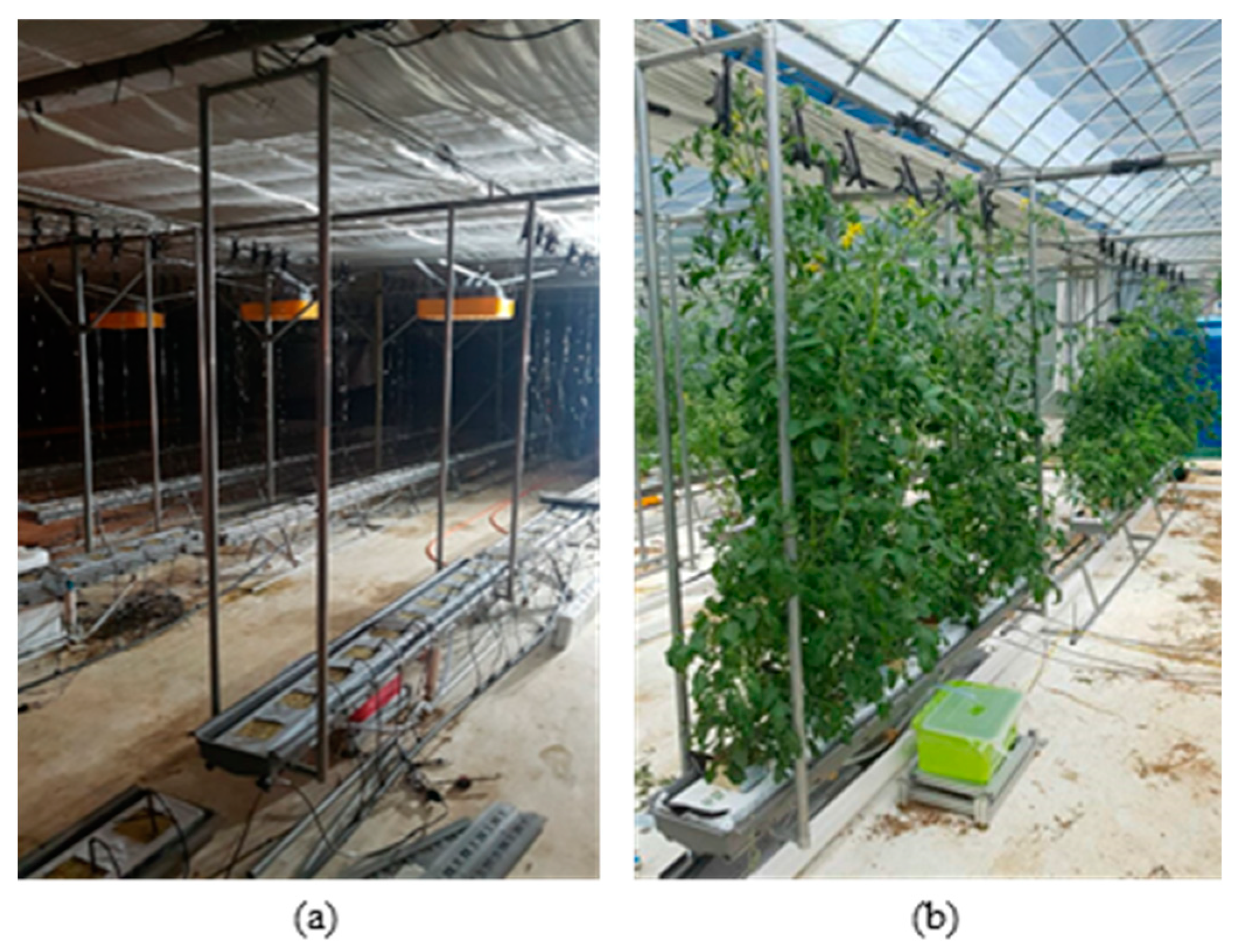
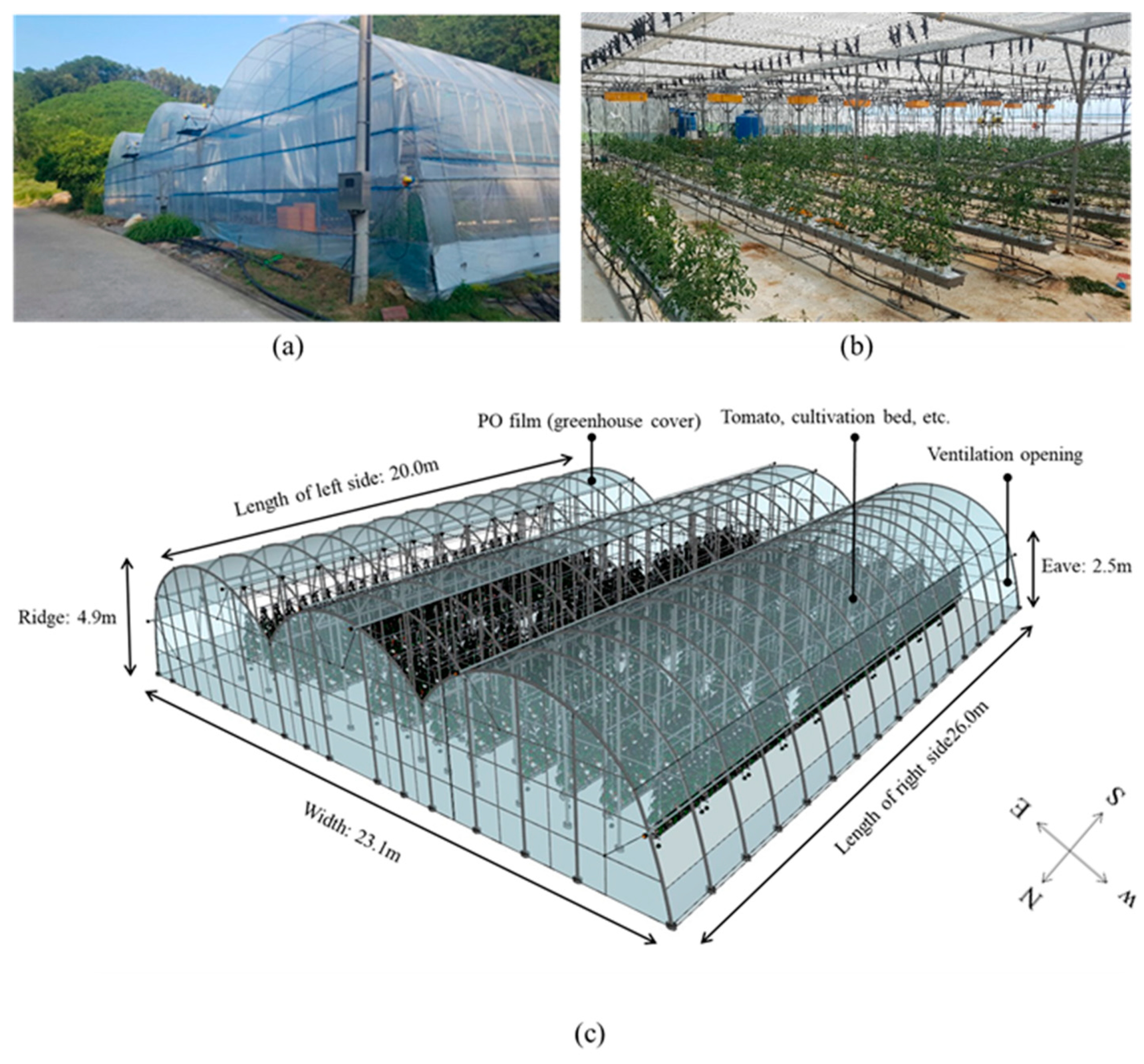
2.1. Experimental Greenhouse

A field experiment to design and then validate the greenhouse BES model and crop model was conducted from 25 May 2018 to 18 August 2018. The experimental greenhouse, which was covered with Polyolefin (PO) film, was located at Andong University (latitude: 36°54′, longitude: 128°80′), Andong-Si, Korea, and was a three-span plastic greenhouse with the following dimensions: 23.1 m wide, 4.5 m high for the ridge, 2.5 m high for the eave, 20.0 m and 26.0 m long (left and right side lengths from the entrance, respectively) (Figure 2). The greenhouse was oriented in the northwest–southwest (NW–SW) direction. A shading net was installed 2.5 m above the ground. Tomatoes (Solanum lycopersicum) were grown in 12 rows, and a total of 560 tomatoes were planted on rock wool cubes and irrigated using a dripper. The amount of irrigation was 100 mL per 80 J cm² accumulated for each tomato. The ventilation of the greenhouse was controlled through the side (side opening of 1.0 m × 20.0 m on the left side and 1.0 m × 25.0 m on the right side) and roof openings of the greenhouse (1.0 m × 20.0 m on the left side and 1.0 m × 25.0 m on the right side shown in Figure 2c. The designed T_a for automatic opening and closing was 20 °C.

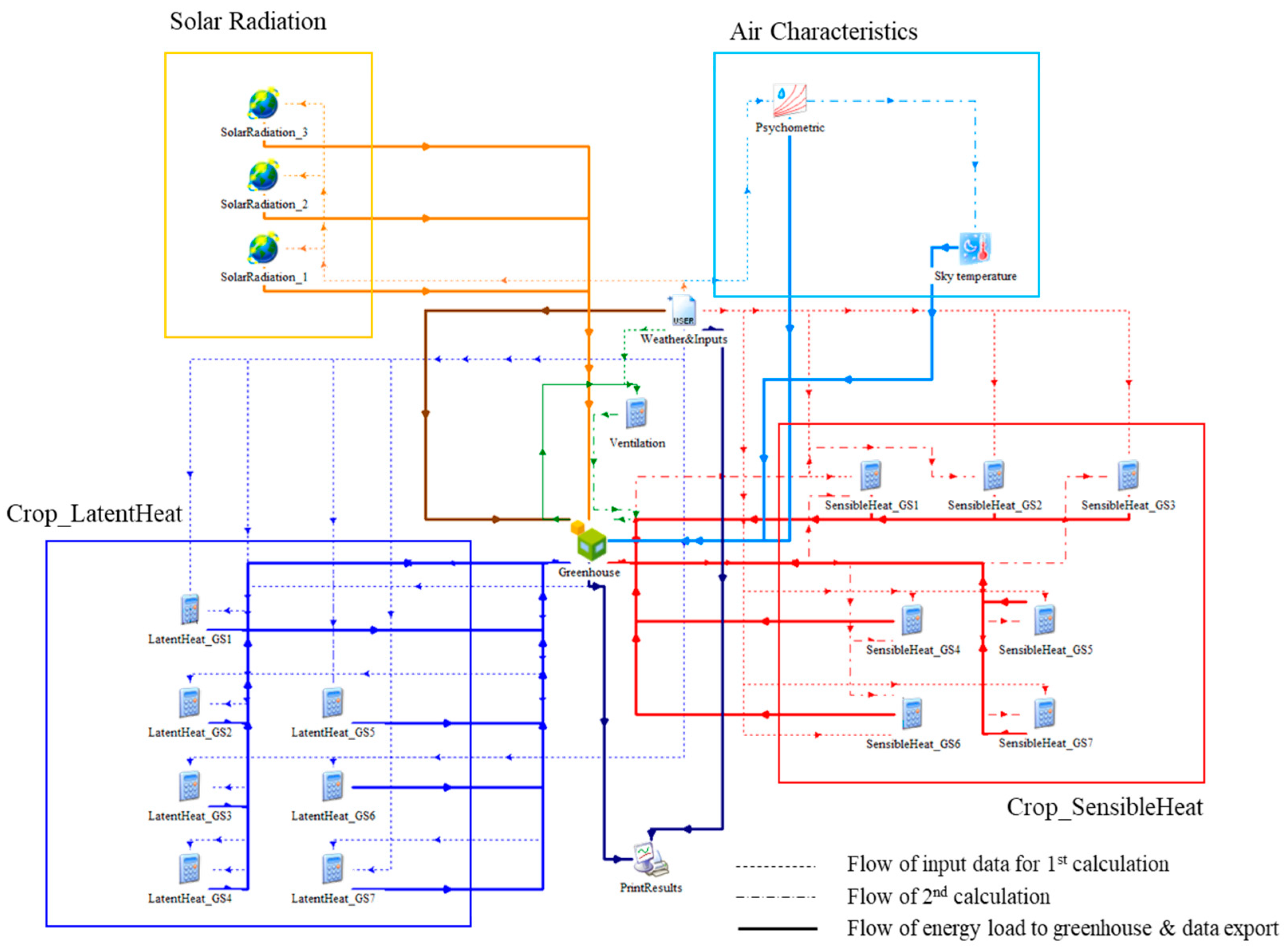
2.2. Bilding Energy Simulation (BES)

BES tools were used to analyse the energy flows of the experimental greenhouse. The BES is a numerical method for calculating the thermal energy flows inside and outside buildings. BES techniques have been used in a variety of fields other than agricultural buildings because they are convenient for designing analytical models and have short computational times. In this study, the commercial software TRNSYS (Transient System Simulation) was used as a tool for greenhouse energy simulation. The TRNSYS software has the advantage of a module-based program, which consists of the main program and several sub-modules to analyse the energy flow of each component. TRNSYS also has the advantage of availability and compatibility on an enormous energy system because of the many sub-modules that can compose various systems such as heat pumps, energy exchange of crops, and ventilation. Based on the energy conservation equation and the transfer function method of the American Society of Heating, Refrigerating and Air-Conditioning Engineers (ASHRAE), the energy exchange inside and outside the building by ventilation, air infiltration, and heat sources were dynamically analysed (Equations (1)–(4)) (TRNSYS User’s Manual, 2018) [58].

$${\dot{Q}}_{\mathrm{i}}={\dot{Q}}_{\mathrm{surf}, \mathrm{i}}+{\dot{Q}}_{\inf , \mathrm{i}}+{\dot{Q}}_{\mathrm{vent}, \mathrm{i}}+{\dot{Q}}_{\mathrm{g}, \mathrm{c}, \mathrm{i}}+{\dot{Q}}_{\mathrm{cplg}, \mathrm{i}}+{\dot{Q}}_{\mathrm{solair}, \mathrm{i}}+{\dot{Q}}_{\mathrm{ISHCCI}, \mathrm{i}}$$

(1)

$${\dot{Q}}_{\inf , \mathrm{i}}=\dot{V}· \rho · c_{\mathrm{p}} \left(T_{\mathrm{outside}, \mathrm{i}}-T_{\mathrm{air}}\right)$$

(2)

$${\dot{Q}}_{\mathrm{vent}, \mathrm{i}}=\dot{V}· \rho · c_{\mathrm{p}} \left(T_{\mathrm{ventilation}, \mathrm{i}}-T_{\mathrm{air}}\right)$$

(3)

$${\dot{Q}}_{\mathrm{cplg}, \mathrm{i}}=\dot{V}· \rho · c_{\mathrm{p}} \left(T_{\mathrm{zone}, \mathrm{i}}-T_{\mathrm{air}}\right)$$

(4)

where ${\dot{Q}}_{\mathrm{surf}, \mathrm{i}}$ is the convective gain from surfaces (kJ), ${\dot{Q}}_{inf, i}$is the infiltration gain (air flow from outside only, kJ), ${\dot{Q}}_{vent, i}$ is the ventilation gains (air flow from a user-defined source, like an HVAC system, kJ), ${\dot{Q}}_{\mathrm{g}, \mathrm{c}, \mathrm{i}}$ is the internal convective gain by people, equipment, illumination, radiators, etc. (kJ), ${\dot{Q}}_{\mathrm{cplg}, \mathrm{i}}$ is the gain due to (convective) air flow from airnode I or the boundary condition (kJ), ${\dot{Q}}_{solair, i}$ is the fraction of solar radiation entering an airnode through external windows, which is immediately transferred as a convective gain to the internal air (kJ), ${\dot{Q}}_{\mathrm{ISHCCI}, \mathrm{i}}$ is the absorbed solar radiation on all internal shading devices of the zone directly transferred as a convective gain to the internal air (kJ), $\dot{V}$ is the target volume (m³), and $c_{\mathrm{p}}$ is specific heat (kJ kg⁻¹ °C⁻¹).

2.3. Computational Fluid Dynamics (CFD)

Computational fluid dynamics (CFD), which numerically calculates the airflow, was used to evaluate the natural ventilation characteristics of the greenhouse. CFD solves the Navier-Stokes equation based on a nonlinear partial differential equation [59,60,61,62,63]. The CFD technique is used to compute the numerical solutions of analysis targets according to various environmental conditions while maintaining the same external environmental conditions. It has the advantage of being able to flexibly design and analyse models, overcoming various limitations of field experiments. Therefore, CFD has been widely used in many industries and research fields such as the aerospace, HVAC, and automotive industries [64]. In this study, the ANSYS Workbench platform (ANSYS Inc., Canonsburg, PA, USA) was used. In the ANSYS Workbench, Design Modeler and ANSYS Meshing (ANSYS Inc., USA) were used to design the geometrical shapes and grids of the numerical model at the pre-processing stage, whereas ANSYS FLUENT (ANSYS Inc., USA) was used to interpret the model under the given boundary conditions.

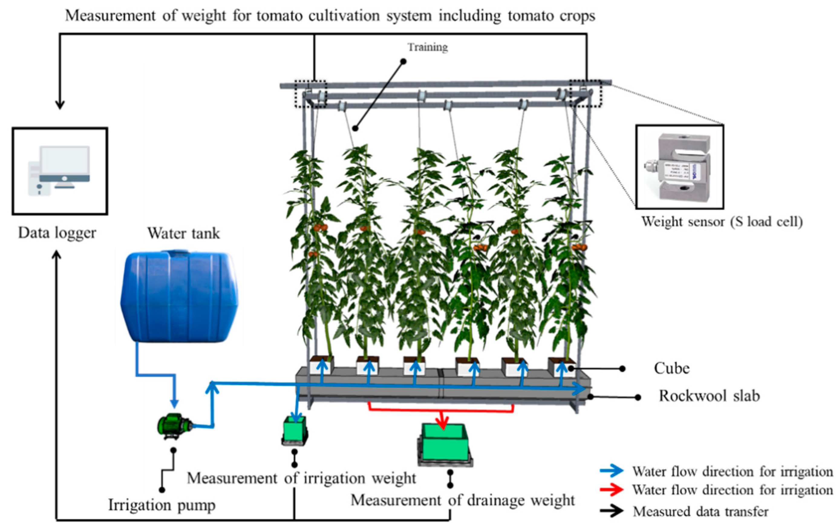
2.4. Experimental Procedures

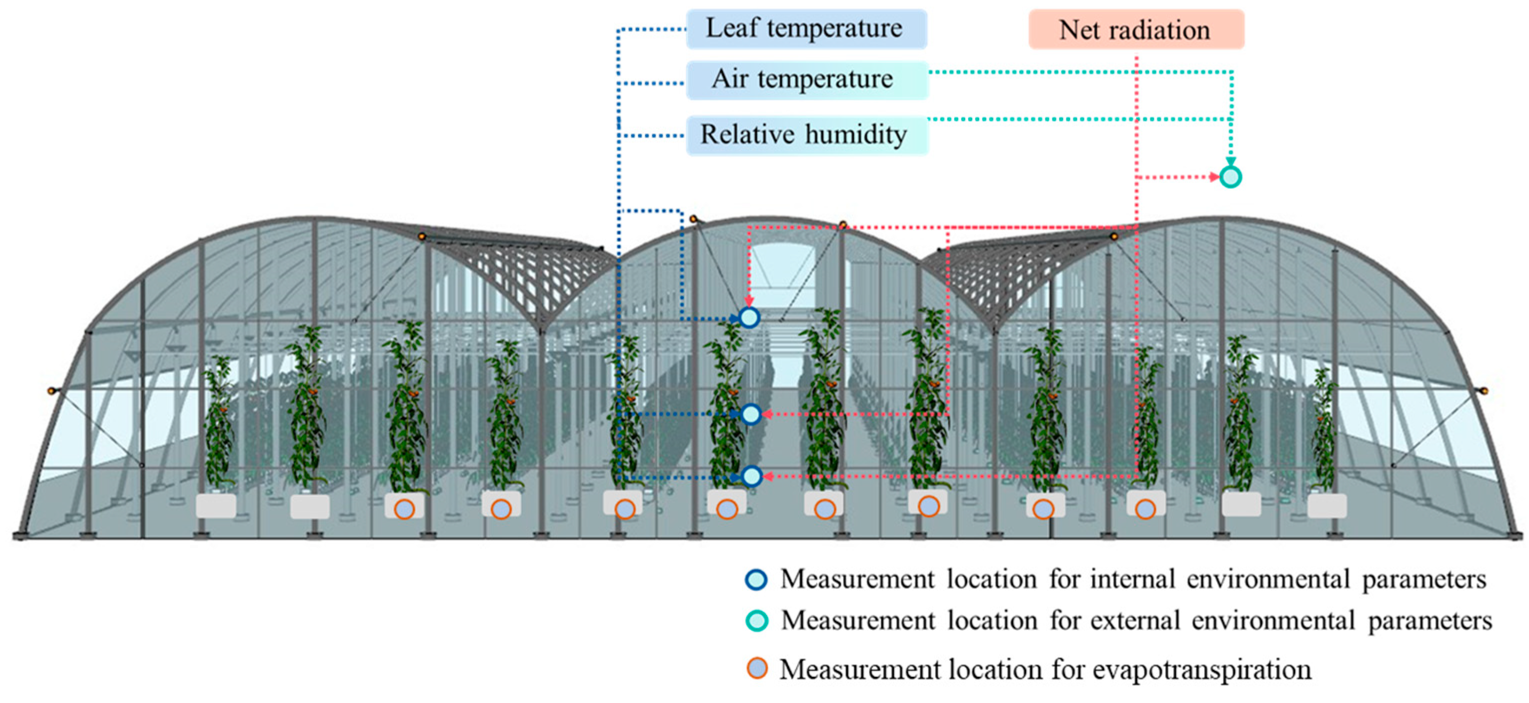
2.4.1. Monitoring of the Environmental Variables

To design and then validate the greenhouse BES model considering the crop (tomato) and natural ventilation characteristics of a greenhouse, a field experiment was conducted from 25 May 2018 to 18 August 2018 in a plastic-covered greenhouse at Andong University. When solar radiation reaches the surface of a leaf, the absorbed energy is partly dissipated by the evaporation (ET) of water (latent heat) and release of sensible heat stored in the products of photosynthesis, and as thermal energy in the leaf body. Solar radiation is nearly equivalent to the sum of sensible and latent heat. Therefore, sensible heat and latent heat were considered. To predict the sensible heat of a crop using Equation (5), measurements of the leaf area index (LAI), leaf temperature (T_L), and T_i were required, and measurement of the amount of ET was essential for predicting latent heat (Equation (6)) [65,66].

$${\mathrm{Q}}_{\mathrm{CS}}=\frac{\mathrm{LAI}·{\mathsf{\rho }}_{\mathrm{a}}·{\mathrm{c}}_{\mathrm{p}}\left({\mathrm{T}}_{\mathrm{L}}-{\mathrm{T}}_{\mathrm{i}}\right)}{{\mathrm{r}}_{\mathrm{a}}}$$

(5)

$${\mathrm{Q}}_{\mathrm{CL}}={\mathsf{\lambda }}_{\mathrm{w}}·\mathrm{ET}$$

(6)

where ${\mathrm{Q}}_{\mathrm{CS}}$ is the sensible heat, ${\mathrm{Q}}_{\mathrm{CL}}$ is the latent heat, $\mathrm{LAI}$ is the leaf area index, ${\mathsf{\rho }}_{\mathrm{a}}$ is the air density (kg m⁻³), ${\mathrm{T}}_{\mathrm{i}}$ is the internal air temperature (°C), ${\mathrm{c}}_{\mathrm{p}}$ is the specific heat of the air (J kg⁻¹ °C⁻¹), ${\mathrm{T}}_{\mathrm{L}}$ is the leaf temperature (°C), ${\mathrm{r}}_{\mathrm{a}}$ is the aerodynamic resistance (s m⁻¹), ${\mathsf{\lambda }}_w$ is the latent heat of vaporization of water (J g⁻¹), and ET is evapotranspiration (g h⁻¹).

RAD, T_i, and RH were monitored both inside and outside the experimental greenhouse. The external weather data were measured by an external weather station (Watchdog 2700 weather station, Spectrum Technologies, Inc., Aurora, IL, USA) which was installed at a place where interference from the surrounding terrain and obstacles (buildings, trees, etc.) was avoided as much as possible. The RAD inside the greenhouse was measured using a pyranometer (sp–510–ss and sp–610–ss, Apogee Instruments, Inc., Logan, UT, USA) and installed in three parts according to the height of the tomato (Figure 3). The T_L was measured at three heights on the tomato using a thermocouple (Thermal–couple, Ondo, Corp., Seoul, Korea) attached to the back surface of the tomato leaf to avoid direct RAD; and the T_i and RH inside the greenhouse were measured at three heights on the tomato using a Hobo sensor (UX100–003, Onset Computer Corp., Bourne, MA, USA). All environmental variables connected to the data-logging system were continuously measured at intervals of five seconds.

Because the ET of tomatoes varies depending on the local environmental conditions inside the greenhouse, monitoring devices for the ET calculation (self–manufactured, Seoul, Korea), as shown in Figure 4, were installed at eight points along the width of the greenhouse (Figure 5). The ET was computed using the water balance equation (Equation (7)). LAI is a dimensionless number that represents the distribution and density of leaves and is defined as the ratio of the total leaf area of a crop to the crop cultivation area. The LAI of the tomato crops was analysed through destruction investigation at 20-day intervals using LI-3100C (LI-COR Inc., Lincoln, NE, USA).

$$\mathrm{ET}=\mathrm{IRR}-\mathrm{DRA}+\Delta \mathrm{BDW}.$$

(7)

where $\mathrm{ET}$ is the evapotranspiration (mL s⁻¹), $\mathrm{IRR}$ is the amount of irrigation (mL s⁻¹), $\mathrm{DRA}$ is the amount of drainage (mL s⁻¹), and $\Delta \mathrm{BDW}$ is the weight increment of the substrate and tomato crop (kg s⁻¹).

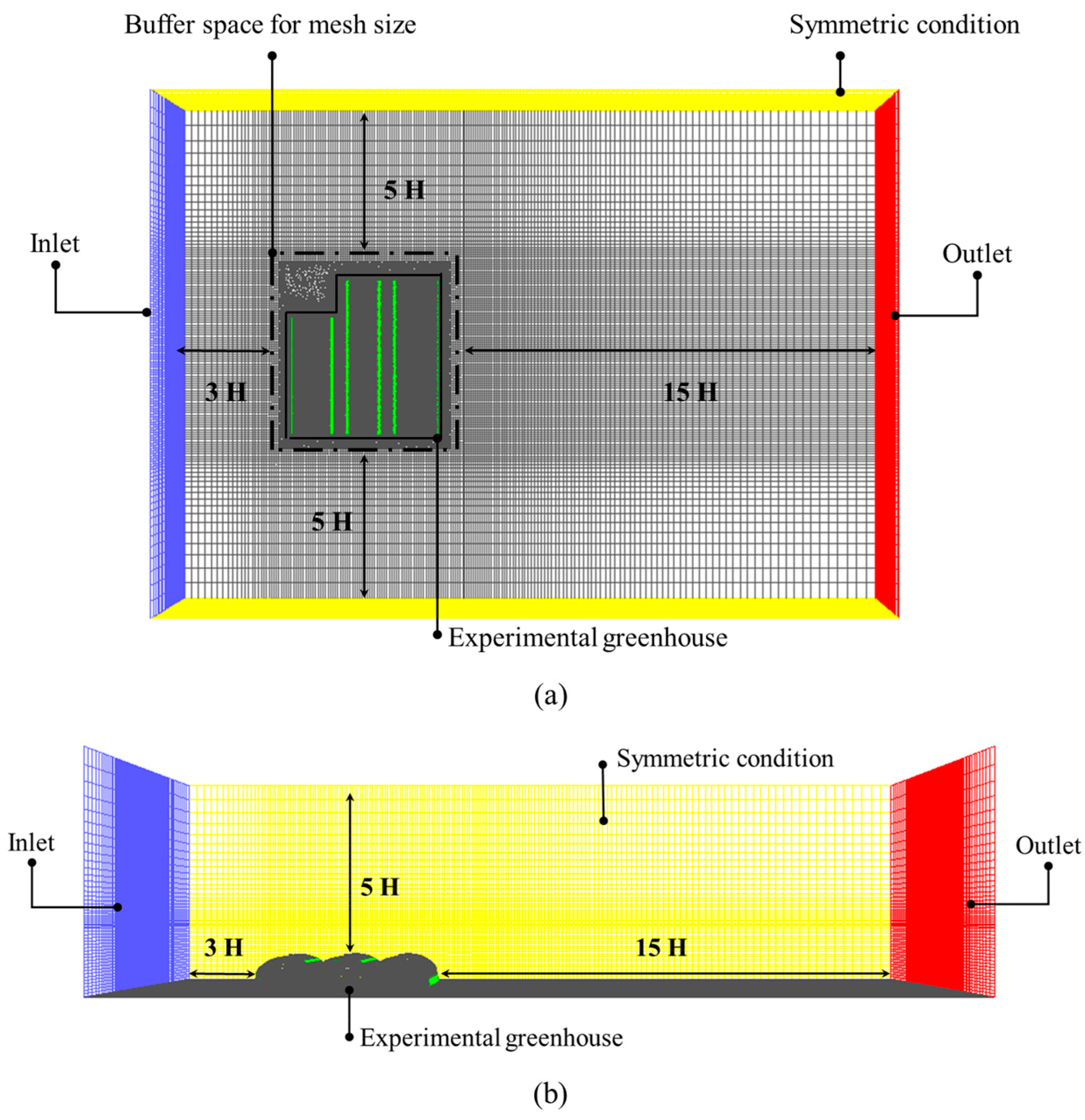
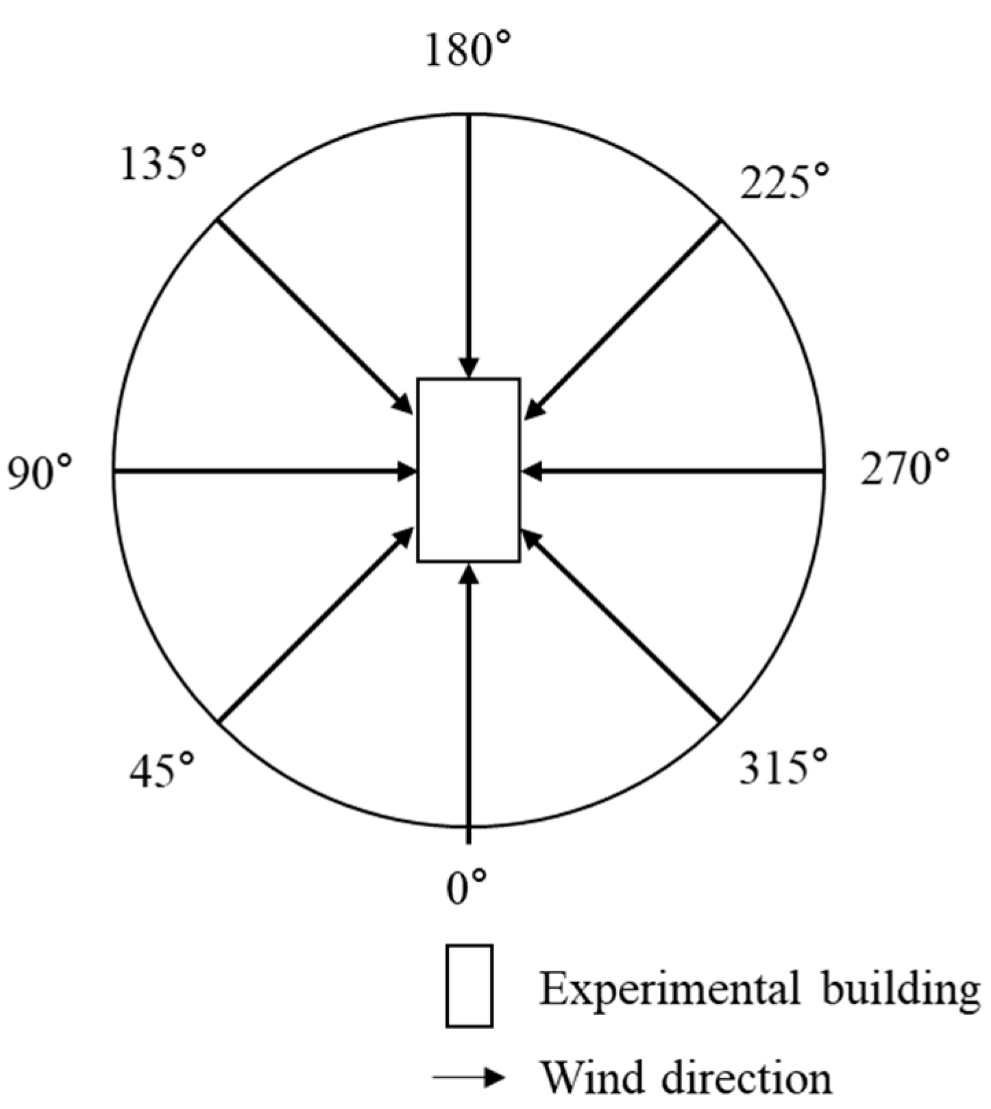
2.4.2. Design of CFD Model to Analyse Ventilation Characteristics of the Experimental Greenhouse

The CFD model for the experimental greenhouse was designed to analyse the natural ventilation characteristics. The design criteria for the external computational domain of the greenhouse presented in the study by Kim et al. (2017) [67] were applied to adequately simulate the external airflow characteristics originating from outside the greenhouse. Kim et al. (2017) [67] stated that the size of the entire computational domain can be determined by the height (H) of the obstacle or target object because the vortex generated at the highest point of the analysis target was first dissipated. Therefore, in this study, according to the height of the greenhouse when the wind blows in a direction perpendicular (90°) to the opening of the greenhouse and parallel to the greenhouse (0°), the size of the computational domain was determined as a windward side, leeward side, side, and top as 3 H, 15 H, 5 H, and 5 H, respectively (Figure 6). In addition, when the wind direction outside the greenhouse originated from 45°, the external computational domain was designed by setting it to 3 H and 15 H at the windward and leeward sides, respectively. Figure 6 showed the top and side views of the computational domain when the wind was generated in a direction perpendicular to the greenhouse (90°) with the greenhouse installed in the north−south direction. The greenhouse CFD model was designed with approximately 5.6 million grids using a hex/prism grid shape. It was designed to satisfy the orthogonal quality (close to 1) and skewness (less than 0.95) criteria required to solve problems with computational errors and accuracy reduction by grid quality.

Because the experimental greenhouse was naturally ventilated, it was important to realize a vertical WS profile considering external obstacles and WS dissipation due to surface roughness. According to the method suggested in the study implemented by Richards (1989) [68], the profiles of average WS, turbulent kinetic energy, and turbulent dissipation rate were applied. The average WS profile was the same as that in Equation (8), and the profiles for the turbulent kinetic energy and turbulent dissipation rate were the same as those in Equations (9) and (10). The RNG k–epsilon turbulence model, which is commonly used to analyse internal fluid interpretation, was applied, and it was validated by Lee et al. (2007) [69] and Bartzanas et al. (2007) [70] that the internal turbulence characteristics of the greenhouse showed high accuracy.

$$U\left(y\right)=\frac{u^{\ast }{}_{ABL}}{k}ln\left(\frac{y+y_0}{y_0}\right)$$

(8)

$$k\left(y\right)=\frac{u^{\ast 2}{}_{ABL}}{\sqrt{C_u}}$$

(9)

$$\epsilon \left(y\right)=\frac{u^{\ast 3}{}_{ABL}}{k\left(y+y_0\right)}$$

(10)

where $\mathrm{u}$ is the average wind speed (m s⁻¹), ${\mathrm{u}}^{\ast }{}_{\mathrm{ABL}}$ is the wall friction velocity (m s⁻¹), k is the von Karman constant (0.42), y is the distance from the wall (m), y₀ is the aerodynamic roughness length (0.03), k is the turbulent kinetic energy (m² s⁻²), C_u is the model fitting parameter (0.09), and ε is the turbulent energy dissipation (m² s⁻³).

A porous media model was developed for the tomatoes inside the greenhouse to account for the effects of crops on the internal climate of the greenhouse. In the CFD model, the Darcy-Forchheimer equation was used as the design formula for the porous media (Equation (11)). The right term of Equation (11) includes the viscous loss and internal energy loss. The viscous loss term was generally negligible in turbulence flows with a Reynolds number of more than 5000 (Equation (12)). Equation (13) was established using the relationship between Equations (11) and (12). L_ad can be calculated by dividing LAI by the height of the tomato crop. The porous media of the CFD model was designed using an average drag coefficient (C_D) of 0.26 for Korea’s representative tomato species derived by Lee et al. (2006) [71,72] and field-measured data (LAI and height of the tomato crop) in this study.

$$\Delta \mathrm{P}=-\left(\frac{\mathsf{\mu }}{\mathsf{\alpha }}\mathrm{v}+{\mathrm{C}}_2\frac{1}{2}{\mathsf{\rho }\mathrm{v}}^2\right)\Delta \mathrm{n}$$

(11)

$$\frac{\Delta \mathrm{P}}{\Delta \mathrm{n}}=-{\mathsf{\rho }\mathrm{L}}_{\mathrm{ad}}{\mathrm{C}}_{\mathrm{D}}{\mathrm{v}}^2$$

(12)

$${\mathrm{C}}_2=2{\mathrm{L}}_{\mathrm{ad}}{\mathrm{C}}_{\mathrm{D}}$$

(13)

where ${\mathrm{C}}_2$ is the inertial resistance factor (m⁻¹), $\mathrm{v}$ is the wind velocity (m s⁻¹), $\mathsf{\alpha }$ is the permeability (m²), $\Delta \mathrm{n}$ is the thickness of the porous medium (m), $\Delta \mathrm{P}$ is the static pressure difference (Pa), $\mathsf{\mu }$ is the viscosity (kg m⁻¹ s⁻¹), ${\mathrm{C}}_{\mathrm{D}}$ is the drag coefficient, and ${\mathrm{L}}_{\mathrm{ad}}$ is the leaf area density (m² m⁻³).

Finally, in the boundary condition (

Table 1. Boundary condition of CFD model of evaluating ventilation characteristics of the greenhouse.

Boundary conditions of the CFD model	Contents	Input Values
	Atmospheric pressure	101,325 Pa
	Density of air	1.225 kg m−3
	Gravitational acceleration	9.81 m s−2
	Inlet	Wind profile (1, 3, 5 m s−1)
	Outlet	Pressure outlet
	Coefficient of viscosity	1.7894 × 10−5
	Drag coefficient of crop	0.26
	Pressure–velocity coupling	SIMPLE algorithm
	Spatial discretization of momentum, volume fraction, turbulent kinetic energy, and turbulence dissipation rate	Second-order upwind
	Spatial discretization of gradient	Least squares cell-based
	Transient formulation	First-order implicit
	Turbulence models	RNG k–ε
	Convergence criteria	$1\times {10}^{-6}$

), the airflow flowing in was defined as the velocity inlet, whereas the airflow flowing out was defined as the pressure outlet. The ground surface of the computational domain was defined as a wall. The boundary conditions on both the side and top surfaces were defined as symmetrical to increase the efficiency of the computation and narrow the extensive space into a finite space. The reference pressure was assumed to be atmospheric pressure, and pressure-based solutions were applied to the solver for interpretation. The SIMPLE algorithm, which provides flexibility and was highly convergent, was used. The previously designed WS profile, turbulent energy, and dissipation rate profile were applied to the inlet of the CFD model, and the standard atmospheric pressure (101,325 Pa) was applied to the outlet. The air density was assumed to be an incompressible ideal gas, and the viscosity was set to 1.7894 × 10⁻⁵ kg m⁻¹ s⁻¹. In addition, it is important to consider the buoyancy effect in a greenhouse because there is a lower wind speed distribution inside the greenhouse than outside the greenhouse. Therefore, the buoyancy effect was activated in the CFD model.

Because the experimental greenhouse was asymmetrical, as shown in Figure 2c, simulation analysis was performed on a total of 108 conditions for eight WD conditions (0°, 45°, 90°, 135°, 180°, 225°, 270°, and 315°), three WS conditions (1.0 m s⁻¹, 3.0 m s⁻¹, and 5.0 m s⁻¹), and four tomato height conditions (no crop, 0.5, 1.0, and 1.6 m).

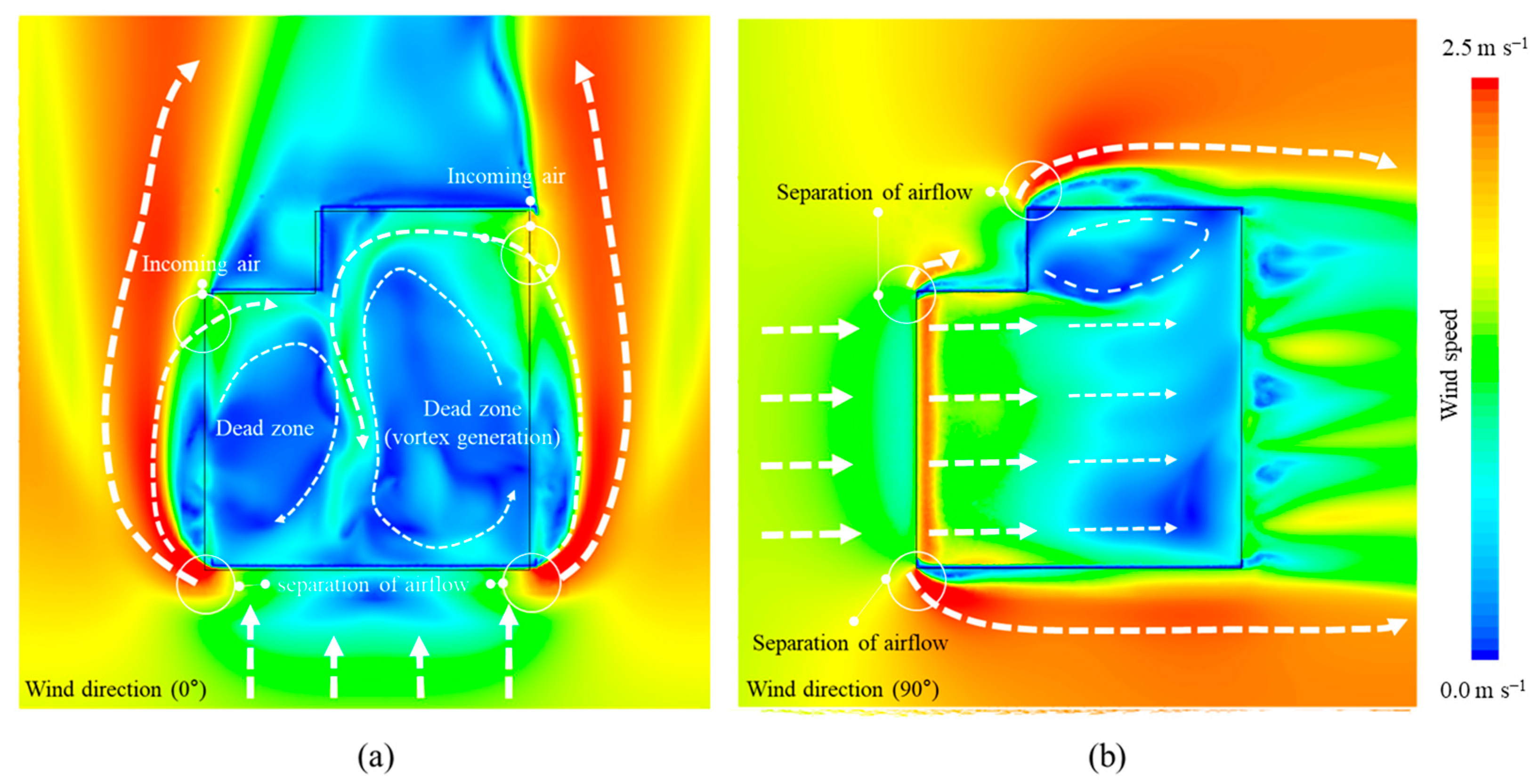
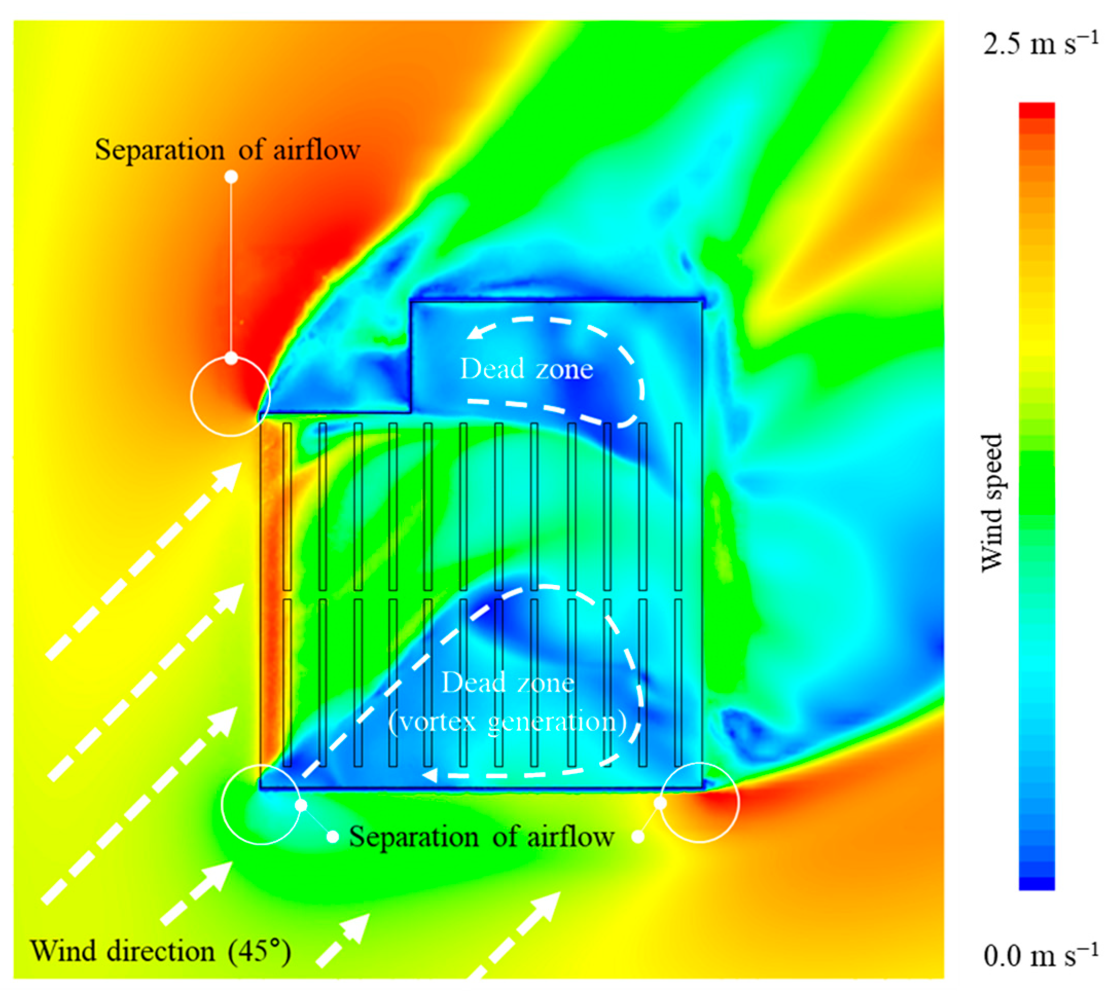
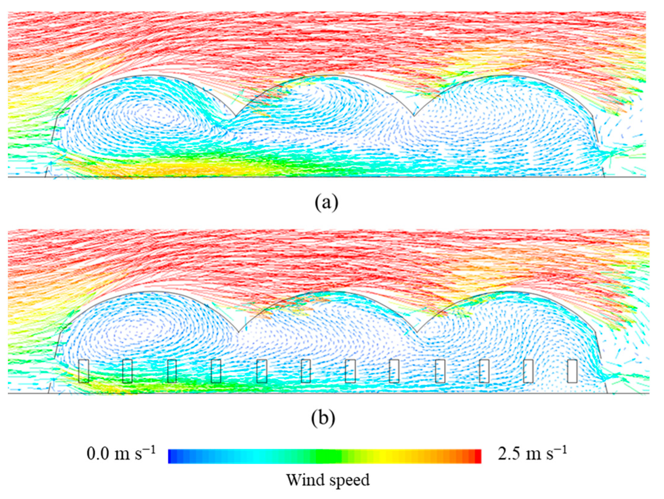
2.4.3. Analysis of CFD-Computed Ventilation Characteristics

The mass flow rate (MFR) method was used to evaluate the natural ventilation rate of the greenhouse (Equation (14)). The MFR can be converted into the number of air changes per hour (ACH), considering the volume of the greenhouse as a unit for quantitatively calculating the natural ventilation rate of the greenhouse, assuming that the amount of air flowing in and out is the same (mass conservation law) (Equation (15)). However, the ventilation rate calculated using the MFR method cannot distinguish between buoyancy-driven ventilation (BDV) and wind-driven ventilation (WDV).

Kittas et al. (1997) [73] presented a numerical model for calculating air change rates considering the BDV and WDV for a naturally ventilated greenhouse with side and roof openings. To calculate the ventilation rate using the proposed equation (Equation (16)), the discharge coefficient (C_d), which depends on the shape of the opening of the greenhouse, height of the tomato, and wind environment (wind direction and speed), should be calculated (Equation (17)). C_d can be calculated using the cross-sectional area of the opening, the difference in the pressure coefficient, and airflow rate (Equation (18)). The calculated C_d was used to calculate the time-dependent change in the ventilation rate of the greenhouse according to the wind environment data. When applying the ventilation rate, Sawachi et al. (2004) [74] assumed that BDV occurred because the WD was parallel to the opening under the conditions of WD 0° and WD 180° (Figure 7). It was also assumed that BDV occurred due to the low effect of the advection under WS of 0.5 m s⁻¹ or less. On the other hand, the WDV was assumed to be dominant when the WS was 1.5 m s⁻¹ or higher because the effect of ventilation by buoyancy was very small. It was assumed that combined WDV and BDV occurred when WS was within the range of 0.5 m s⁻¹ to 1.5 m s⁻¹.

$$\mathrm{MFR} \left(\mathrm{Q}\right)=\mathsf{\rho }\times \mathrm{U}\times \mathrm{A}$$

(14)

$$ACH=\frac{Q}{\left(\rho \times V\right)}$$

(15)

$$Q=C_d{\left[{\left(\frac{A_R{A}_S}{\sqrt{A_R{}^2+A_S{}^2}}\right)}^2\left(2g\frac{\Delta T}{T_0}h\right)+{\left(\frac{A_T}{2}\right)}^2{C}_w{u}^2\right]}^{0.5}$$

(16)

$$={\mathrm{C}}_{\mathrm{d}}\mathrm{A}\sqrt{\frac{2\Delta \mathrm{P}}{\mathsf{\rho }}}$$

(17)

$${\mathrm{C}}_{\mathrm{d}}=\frac{\mathrm{Q}}{\mathrm{A}\times \mathrm{V}\times \sqrt{\left({\mathrm{C}}_{\mathrm{p}1}-{\mathrm{C}}_{\mathrm{p}2}\right)}}$$

(18)

where MFR is the mass flow rate (kg s⁻¹), $\mathsf{\rho }$ is the air density (kg m⁻³), $\mathrm{U}$ is the air velocity (m s⁻¹), A is the area (m²), ACH is the air change rate (h⁻¹), V is the volume of the experimental facility (m³), P_ref is the reference pressure (Pa), $\mathsf{\rho }$ is the air density (kg m⁻³), ${\mathrm{V}}_{\mathrm{ref}}$ is the wind speed at reference height (m s⁻¹), P₁ and P₂ are the pressures (Pa), ${\mathrm{C}}_{\mathrm{p}1}$ and ${\mathrm{C}}_{\mathrm{p}2}$ are the wind pressure coefficients inside and outside the greenhouse, ${\mathrm{C}}_{\mathrm{d}}$ is the discharge coefficient, $\mathrm{A}$ is the area of opening (m²), $\mathrm{V}$ is the wind speed (m s⁻¹), Q is the ventilation rate (m³ s⁻¹), T_i is the internal air temperature (K), T_o is the external air temperature (K), A_R is the total opening area of the roof vents (m²), As is the total opening area of the side vent (m²), A_T is the total opening area of all the vents (=A_r + A_s) (m²), and g is the acceleration due to gravity (9.81 m s⁻²). The equation applies when T_i > T_o. If T_i < T_o, T_i in the denominator is replaced by T_o, and (T_i − T_o) in the numerator is replaced by (T_e − T_i).

2.4.4. Design and Validation of the Greenhouse BES Model Integrated with the Tomato Crop Model and Ventilation Characteristics

To design and then validate the greenhouse BES model considering the crop (tomato) and natural ventilation characteristics of a greenhouse, the greenhouse BES model was designed using the modules of TRNSYS software (Ver. 18), such as a data reader (Type 9) that inputs hourly external weather data and internal climate data (T_a, RH, surface temperature, RAD, atmospheric pressure), radiation processor (Type 16), psychrometric calculator (Type 69), sky temperature calculator (Type 33), multizone building (Type 56), user-defined function, and reporter. Using the TRNSys3D plug-in of TRNSYS, a three-dimensional structure (Type 56) of the experimental greenhouse was designed using SketchUp 2018 (Trimble Inc., Sunnyvale, CA, USA). Unlike typical buildings, plastic greenhouses are usually made of very thin vinyl material, and the covering characteristics of the greenhouse that can be interconnected with TRNSYS were designed using the Window 7.3 software used by Lee et al. (2012) [26] (

Table 2. Properties of the covering material for the experimental greenhouse [26].

Parameters	Input Values
Solar transmittance	0.862
Solar reflectance (exterior and interior facing side)	0.105
Visible transmittance	0.881
Visible reflectance (exterior and interior facing side)	0.108
Thermal infrared transmittance	0
Infrared emittance (exterior and interior facing side)	0.658
Conductivity (W m−1 K−1)	0.14
U factor (W m−2 K−1)	5.412

).

Inside the experimental greenhouse, the vent openings were operated according to the internal environment (Equation (19)). The vent was designed to open when the internal air temperature was higher than the external air temperature, and the internal air temperature was higher than the internal designed air temperature; whereas it was designed to close when the internal air temperature was lower than the designed internal air temperature. The operating conditions for all the equipment were measured through field experiments and then input as a boundary condition into the greenhouse BES model. The tomato crop model, depending on the growth stage of the tomatoes (seven stages), was designed using a calculator module. In the greenhouse BES model, the ventilation characteristics of the greenhouse were designed in the same manner as the control logic operated in the actual cultivation environment. When the RAD of 800 W m⁻² or more was monitored in the greenhouse, the shading net inside the greenhouse was used. Furthermore, the ventilation rate applied to the BES model was computed using CFD.

$$\mathrm{VENTSIGN}=\{\begin{array}{cc}1& \left({\mathrm{T}}_{\mathrm{i}}>{\mathrm{VENTTEMP} \mathrm{and} \mathrm{T}}_{\mathrm{i}}>{\mathrm{T}}_{\mathrm{o}}\right)\\ 0& \left({\mathrm{T}}_{\mathrm{i}}\le \mathrm{VENTTEMP}\right)\end{array}$$

(19)

where $\mathrm{VENTSIGN}$ is the ventilation signal, $\mathrm{VENTTEMP}$ is the set temperature of the ventilation, ${\mathrm{T}}_{\mathrm{i}}$ is the internal air temperature (°C), and ${\mathrm{T}}_{\mathrm{o}}$ is the external air temperature (°C).

The BES model was validated using the standard error and coefficient of determination (R²) from the T_a measured inside the greenhouse [75,76,77,78]. The T_a and RH values computed using the greenhouse BES model were validated using field-measured T_a and RH data measured from 9 June 2018 to 15 August 2018. In addition, to determine the suitability of the tomato crop model as an individual module, the estimated ET and T_L with the designed tomato crop model were validated by comparing the measured ET and T_L.

3. Results and Discussion

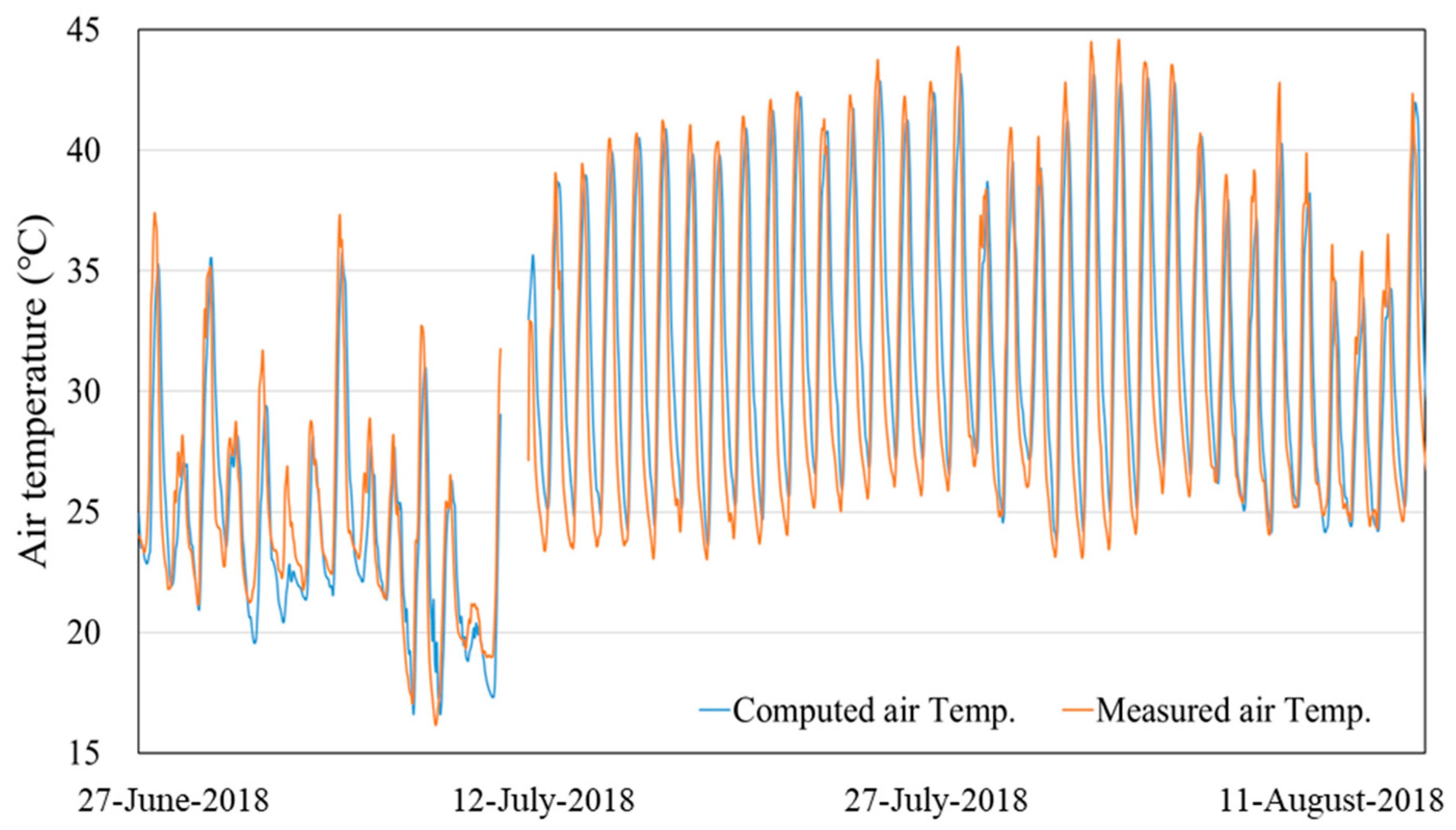
3.1. Environmental Monitoring Inside and Outside the Greenhouse

Table 3. Monitoring of micro-climate environment in the greenhouse (from 25 May 2018 to 18 August 2018).

Classification	Average	Highest	Lowest	SD
Internal air temperature (°C)	27.4	45.3	16.3	6.2
External air temperature (°C)	25.0	34.7	12.1	4.8
Leaf temperature (°C)	26.8	44.1	16.6	5.7
Internal relative humidity (%)	91.1	100	29.3	7.5
External relative humidity (%)	82.6	100	46.3	8.1
Internal solar radiation (W m−2)	–	629.4	0.0	–
External solar radiation (W m−2)	–	969.4	0.0	–

showed the field-measured data for the average T_a, RH, and RAD inside and outside the greenhouse during the entire experimental period. The average T_i and standard deviation (SD) of the greenhouse were 27.4 °C and 6.2 °C, respectively, while the RH was 91.1% (SD: 7.5%). At night, when T_o was lower than T_set inside the greenhouse, the internal RH reached a maximum of 100%. This is because the vent openings were closed, resulting in an increase in internal moisture. However, during the daytime, the average T_i of the greenhouse was 30.5 °C (SD: 6.1 °C). During the daytime, the average T_i of the greenhouse increased by 28.1% owing to radiative heat transfer and convective heat transfer caused by RAD, while the RH decreased by 8.0% compared to the daily average value.

During the entire experimental period, the average T_L was 26.8 °C (SD: 5.7 °C). There was no significant difference (only 0.6 °C) between the internal T_a of the greenhouse and T_L. Even at night, the average T_L was 23.9 °C (SD: 3.6 °C), which did not significantly differ from the ambient T_i. On the other hand, the T_L during the daytime was 5.5 °C higher than that at night, 29.4 °C (SD: 5.9 °C). Therefore, during the daytime, it was determined that the change in sensible heat and latent heat energy would be significant owing to the evapotranspiration of the tomato crop affecting the T_L.

The highest external RAD was 969.4 W m⁻², and the internal RAD was in the range of 0–629.4 W m⁻² during the experimental period. The decrease in internal RAD generated by passing through the greenhouse-covering material was 35.1% on average. This was because dust accumulated on the covering material as the usage period of the greenhouse covering material elapsed, or the covering material was contaminated with other substances and was damaged by opening and closing the side and roof openings of the greenhouse [79].

The RAD and internal T_a are factors that greatly affect the ET of crops. The ET for each tomato plant varied according to the internal and external environmental conditions of the greenhouse. The ET for each tomato plant was 2.8 g plant⁻¹ per hour on average, and up to 18.7 g plant⁻¹ h⁻¹. When the T_L was higher than the ambient T_i, the ET increased to control the excessive temperature rise within the tomato leaf.

The tomato LAI measured through the destruction investigation was shown in Figure 8. It increased with the number of cultivation days, and leaf area and plant height increased exponentially at the beginning of planting. This was similar to the results measured through field experiments by Monte et al. (2013) [80], in which a sigmoid curve was generated for the period after planting tomatoes. As the cultivation days elapsed, the change in the LAI of tomatoes was 1.1 at the initial stage and 5.2 at maximum growth (4 June 2018 to 18 September 2018). A value greater than the LAI of 5.2 was rarely generated due to aged leaf care and tomato height adjustments, and the LAI was maintained at 5.2.

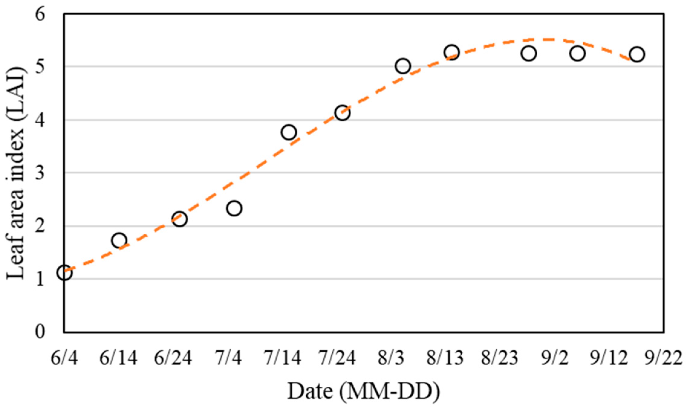
3.2. Design and Validation of Crop Model

To analyse the correlation of environmental variables measured in the experimental greenhouse and then design the tomato crop model, the average value of the field-measured data for each variable was used.

Table 4. Pearson correlation analysis for environmental variables (ET, T_i, RH, T_L, RAD) of the greenhouse.

Parameters		ET	Ti	RH	TL	RAD
ET	Pearson correlation	1	0.611 **	−0.605 **	0.453 **	0.729 **
	Significance probability		0.000	0.000	0.000	0.000
Ti	Pearson correlation	0.611 **	1	−0.701 **	0.967 **	0.671 **
	Significance probability	0.000		0.000	0.000	0.000
RH	Pearson correlation	−0.605 **	−0.701 **	1	−0.681 **	−0.622 **
	Significance probability	0.000	0.000		0.000	0.000
TL	Pearson correlation	0.453 **	0.967 **	−0.681 **	1	0.613 **
	Significance probability	0.000	0.000	0.000		0.000
RAD	Pearson correlation	0.729 **	0.671 **	−0.622 **	0.613 **	1
	Significance probability	0.000	0.000	0.000	0.000

** Correlation is significant at the 0.01 level.

showed the results of the analysis of the Pearson correlation between environmental variables (T_i, T_L, and RH). The measured ET and RAD, T_i, RH, and T_L were found to have correlations of 0.73, 0.61, −0.605, and 0.45, respectively, and were found to be significant at a confidence level of 0.01%. RAD, T_i, and T_L were positively correlated with ET, whereas RH was negatively correlated. Although the correlation between the T_i and RH of the greenhouse and T_L did not show a strong correlation, the ET of tomato crops was found to have the greatest correlation with the RAD, and a weak positive correlation between T_i and T_L was found.

The microclimate environment (T_i, RH, RAD) that was distributed inside the greenhouse caused a change in the T_L of the tomato crop and a difference in the ET of tomatoes due to time-dependent changes. Therefore, a multiple regression model was designed to predict T_L and ET from microclimate environmental variables inside the greenhouse. The growth of tomatoes during the cultivation period showed a curve similar to a sigmoid curve and had a significant effect on the energy model (Figure 8). Changes in LAI by cultivation day after planting can be mathematically expressed using Equation (20) in the form of a cubic equation (R² = 0.98). In this study, the growth stages after planting tomatoes in a greenhouse were divided into seven stages, and multiple regression models for T_L and ET were designed. The stages of crop growth were divided into two-week intervals, similar to the destruction investigation of the tomato crop. The designed regression model was applied to consider the tomato energy-exchange characteristics in the greenhouse BES model. The multiple regression equations for estimating T_L and ET were designed according to the tomato growth stages, as shown in Table 5 and Table 6.

$$\mathrm{Y}=9\times {10}^{-6}{\left(\mathrm{day}\right)}^3+0.0012{\left(\mathrm{day}\right)}^2+0.018\left(\mathrm{day}\right)+0.841$$

(20)

(If, day ≥ 20, R² = 0.98)

The correlation (R) between the evapotranspiration of tomatoes estimated through multiple regression equations and evapotranspiration measured through field experiments was 0.74. The average error between the ET estimated using the multiple regression model and the field-measured ET was 0.95 g h⁻¹ on average. In addition, the correlation between the estimated and measured leaf temperatures using the multiple regression model was 0.98. The absolute error between the estimated T_L and measured T_L was 0.7 °C. Finally, the designed T_L estimation model was applied to calculate the sensible heat (Equation (21)), and the ET estimation model was applied to calculate the latent heat of tomatoes (Equation (22)) in the greenhouse BES model.

$${\mathrm{Q}}_{\mathrm{CS}}=\frac{\mathrm{f}(\mathrm{day})·{\mathsf{\rho }}_{\mathrm{a}}·{\mathrm{C}}_{\mathrm{p}}\left(\mathrm{f}\left({\mathrm{T}}_{\mathrm{i}}, \mathrm{H},{ \mathrm{R}}_{\mathrm{s}}\right)-{\mathrm{T}}_{\mathrm{a}}\right)}{{\mathrm{r}}_{\mathrm{a}}}$$

(21)

$${\mathrm{Q}}_{\mathrm{CL}}=\mathsf{\lambda }·\mathrm{f}\left({\mathrm{T}}_{\mathrm{i}}, \mathrm{H},{\mathrm{T}}_{\mathrm{L}},{\mathrm{R}}_{\mathrm{s}}\right)$$

(22)

where ${\mathrm{Q}}_{\mathrm{CS}}$ is the sensible heat of the crop; ${\mathrm{Q}}_{\mathrm{C}L}$ is the latent heat of the crop; f(d) is the LAI function according to the number of days after planting,${ \mathsf{\rho }}_{\mathrm{a}}$ is the air density (kg m⁻³), ${\mathrm{C}}_{\mathrm{p}}$ is the specific heat of the air (J kg⁻¹ °C⁻¹), f (T, H, R) is the function of estimating leaf temperature, ${\mathrm{T}}_{\mathrm{i}}$ is the air temperature inside the greenhouse, ${\mathrm{r}}_{\mathrm{a}}$ is the aerodynamic resistance (s m⁻¹), $\mathsf{\lambda }$ is the latent heat of vaporization of water (J g⁻¹), and f (T, H, T_L, R) is the function of estimating evapotranspiration (g h⁻¹),${ \mathrm{r}}_{\mathrm{a}}=840{\left(\frac{\mathrm{l}}{\left|{\mathrm{T}}_{\mathrm{o}}-{\mathrm{T}}_{\mathrm{a}}\right|}\right)}^{0.25}$,$\mathrm{l}$ is the leaf dimension (m), and ${\mathrm{T}}_{\mathrm{o}}$ is the ambient air temperature (°C).

Table 5. Multiple regression model for estimating ET by growth stages.

Stage	The Equation for Estimating ET of Tomato	Adjusted R2	Pr > |t|	Equations
1	${\mathrm{ET}}_1=-91.452+8.674{\mathrm{T}}_{\mathrm{i}}+0.332\mathrm{RH}-5.743{\mathrm{T}}_{\mathrm{L}}+0.207\mathrm{RAD}$	0.909	<0.001	(23)
2	${\mathrm{ET}}_2=282.257+6.31{\mathrm{T}}_{\mathrm{i}}-2.58\mathrm{RH}-7.786{\mathrm{T}}_{\mathrm{L}}+0.276\mathrm{RAD}$	0.876	<0.001	(24)
3	${\mathrm{ET}}_3=252.151-5.64{\mathrm{T}}_{\mathrm{i}}-2.602\mathrm{RH}+5.741{\mathrm{T}}_{\mathrm{L}}+0.443\mathrm{RAD}$	0.886	<0.001	(25)
4	${\mathrm{ET}}_4=173.53+8.992{\mathrm{T}}_{\mathrm{i}}-1.546\mathrm{RH}-9.838{\mathrm{T}}_{\mathrm{L}}+0.109\mathrm{RAD}$	0.719	<0.001	(26)
5	${\mathrm{ET}}_5=-32.525+0.474{\mathrm{T}}_{\mathrm{i}}+0.207\mathrm{RH}+0.117{\mathrm{T}}_{\mathrm{L}}+0.18\mathrm{RAD}$	0.833	<0.001	(27)
6	${\mathrm{ET}}_6=34.738+1.416{\mathrm{T}}_{\mathrm{i}}-0.507\mathrm{RH}-0.689{\mathrm{T}}_{\mathrm{L}}+0.164\mathrm{RAD}$	0.878	<0.001	(28)
7	${\mathrm{ET}}_7=229.251-4.787{\mathrm{T}}_{\mathrm{i}}-2.171\mathrm{RH}+4.009{\mathrm{T}}_{\mathrm{L}}+0.135\mathrm{RAD}$	0.974	<0.001	(29)

Table 5. Multiple regression model for estimating ET by growth stages.

Stage	The Equation for Estimating ET of Tomato	Adjusted R2	Pr > |t|	Equations
1	${\mathrm{ET}}_1=-91.452+8.674{\mathrm{T}}_{\mathrm{i}}+0.332\mathrm{RH}-5.743{\mathrm{T}}_{\mathrm{L}}+0.207\mathrm{RAD}$	0.909	<0.001	(23)
2	${\mathrm{ET}}_2=282.257+6.31{\mathrm{T}}_{\mathrm{i}}-2.58\mathrm{RH}-7.786{\mathrm{T}}_{\mathrm{L}}+0.276\mathrm{RAD}$	0.876	<0.001	(24)
3	${\mathrm{ET}}_3=252.151-5.64{\mathrm{T}}_{\mathrm{i}}-2.602\mathrm{RH}+5.741{\mathrm{T}}_{\mathrm{L}}+0.443\mathrm{RAD}$	0.886	<0.001	(25)
4	${\mathrm{ET}}_4=173.53+8.992{\mathrm{T}}_{\mathrm{i}}-1.546\mathrm{RH}-9.838{\mathrm{T}}_{\mathrm{L}}+0.109\mathrm{RAD}$	0.719	<0.001	(26)
5	${\mathrm{ET}}_5=-32.525+0.474{\mathrm{T}}_{\mathrm{i}}+0.207\mathrm{RH}+0.117{\mathrm{T}}_{\mathrm{L}}+0.18\mathrm{RAD}$	0.833	<0.001	(27)
6	${\mathrm{ET}}_6=34.738+1.416{\mathrm{T}}_{\mathrm{i}}-0.507\mathrm{RH}-0.689{\mathrm{T}}_{\mathrm{L}}+0.164\mathrm{RAD}$	0.878	<0.001	(28)
7	${\mathrm{ET}}_7=229.251-4.787{\mathrm{T}}_{\mathrm{i}}-2.171\mathrm{RH}+4.009{\mathrm{T}}_{\mathrm{L}}+0.135\mathrm{RAD}$	0.974	<0.001	(29)

Table 6. Multiple regression model for estimating T_L by growth stages.

Stage	The Equation for Estimating TL of Tomato	Adjusted R2	Pr > |t|	Equations
1	${\mathrm{T}}_{\mathrm{L}}=4.342+0.724{\mathrm{T}}_{\mathrm{i}}+0.013\mathrm{RH}-0.005\mathrm{RAD}$	0.963	<0.001	(30)
2	${\mathrm{T}}_{\mathrm{L}}=1.211+0.782{\mathrm{T}}_{\mathrm{i}}+0.033\mathrm{RH}-0.006\mathrm{RAD}$	0.968	<0.001	(31)
3	${\mathrm{T}}_{\mathrm{L}}=7.338+0.849{\mathrm{T}}_{\mathrm{i}}-0.042\mathrm{RH}-0.003\mathrm{RAD}$	0.972	<0.001	(32)
4	${\mathrm{T}}_{\mathrm{L}}=7.723+0.943{\mathrm{T}}_{\mathrm{i}}-0.065\mathrm{RH}$	0.977	<0.001	(33)
5	${\mathrm{T}}_{\mathrm{L}}=0.905+0.894{\mathrm{T}}_{\mathrm{i}}+0.017\mathrm{RH}-0.003\mathrm{RAD}$	0.992	<0.001	(34)
6	${\mathrm{T}}_{\mathrm{L}}=2.686+0.947{\mathrm{T}}_{\mathrm{i}}-0.016\mathrm{RH}-0.004\mathrm{RAD}$	0.995	<0.001	(35)
7	${\mathrm{T}}_{\mathrm{L}}=12.387+0.835{\mathrm{T}}_{\mathrm{i}}-0.088\mathrm{RH}-0.006\mathrm{RAD}$	0.993	<0.001	(36)

Table 6. Multiple regression model for estimating T_L by growth stages.

Stage	The Equation for Estimating TL of Tomato	Adjusted R2	Pr > |t|	Equations
1	${\mathrm{T}}_{\mathrm{L}}=4.342+0.724{\mathrm{T}}_{\mathrm{i}}+0.013\mathrm{RH}-0.005\mathrm{RAD}$	0.963	<0.001	(30)
2	${\mathrm{T}}_{\mathrm{L}}=1.211+0.782{\mathrm{T}}_{\mathrm{i}}+0.033\mathrm{RH}-0.006\mathrm{RAD}$	0.968	<0.001	(31)
3	${\mathrm{T}}_{\mathrm{L}}=7.338+0.849{\mathrm{T}}_{\mathrm{i}}-0.042\mathrm{RH}-0.003\mathrm{RAD}$	0.972	<0.001	(32)
4	${\mathrm{T}}_{\mathrm{L}}=7.723+0.943{\mathrm{T}}_{\mathrm{i}}-0.065\mathrm{RH}$	0.977	<0.001	(33)
5	${\mathrm{T}}_{\mathrm{L}}=0.905+0.894{\mathrm{T}}_{\mathrm{i}}+0.017\mathrm{RH}-0.003\mathrm{RAD}$	0.992	<0.001	(34)
6	${\mathrm{T}}_{\mathrm{L}}=2.686+0.947{\mathrm{T}}_{\mathrm{i}}-0.016\mathrm{RH}-0.004\mathrm{RAD}$	0.995	<0.001	(35)
7	${\mathrm{T}}_{\mathrm{L}}=12.387+0.835{\mathrm{T}}_{\mathrm{i}}-0.088\mathrm{RH}-0.006\mathrm{RAD}$	0.993	<0.001	(36)

3.3. Evaluation of Ventilation Rate According to Wind Environment and Crops

Table 7. CFD-computed ACH of the greenhouse according to WD, WS, and crop height conditions.

Categories		Wind Direction (°)
Wind Speed (m s−1)	Tomato Canopy	0	45	90	135	180	225	270	315
1.0	No crop	6.12	15.73	18.08	14.98	5.61	16.18	18.52	17.47
	0.5 m	6.38	14.57	15.26	13.31	5.40	15.40	17.07	16.32
	1.0 m	6.51	14.55	15.01	13.27	5.64	14.73	17.02	15.89
	1.6 m	6.72	14.43	14.93	13.36	5.44	14.36	17.30	15.49
3.0	No crop	11.46	43.74	50.11	43.08	13.98	46.51	54.15	48.87
	0.5 m	10.57	42.60	47.55	41.77	10.36	44.10	54.00	46.88
	1.0 m	10.24	40.63	47.25	40.84	10.49	41.27	53.86	46.99
	1.6 m	9.93	39.05	45.65	40.50	11.14	41.21	53.38	46.92
5.0	No crop	16.77	73.14	82.92	72.05	26.48	78.06	94.15	82.27
	0.5 m	15.97	71.35	80.15	70.66	23.34	74.61	91.79	79.66
	1.0 m	15.30	67.76	78.77	67.69	22.65	70.80	90.36	78.98
	1.6 m	15.24	65.63	77.07	67.60	20.69	69.57	88.51	77.36

indicated the CFD-computed ventilation rates of the greenhouse according to the external WD, WS, and height of the tomato crops. Depending on the conditions for scenario analysis, at least 5.4 ACH and up to 94.15 ACH had occurred. Albright (1990) [81] and Lindley and Whitaker (1996) [82] suggested ventilation rates from 45.0 ACH to 60.0 ACH for commercial greenhouses to keep the T_i of the greenhouse within 5 °C of the T_o in the summer. Considering the recommended ventilation rate (ventilation requirement) in a greenhouse, the CFD-computed results confirmed that the ventilation rate did not meet the ventilation requirements based on the WD, WS, and tomato height conditions. In particular, in many studies related to calculating the energy loads for a greenhouse, 0.7 ACH or slightly larger ACH (fixed value) was applied, or a ventilation rate of 45.0–60.0 ACH was applied considering the ventilation characteristics. In this case, the energy load of the BES model may be overestimated or underestimated over the season. It may also provide inaccurate results for the design capacity of the system for environmental control.

The ventilation rates of the greenhouse varied depending on the direction of the external air (WD conditions), wind speed (WS), crop, ventilation devices, etc. For WD conditions, when the external WD was oriented perpendicular to the opening of the greenhouse (WD 90° and 270° in this study), the ventilation rate was relatively high compared to other WD conditions. Conversely, when generated along the parallel direction with the opening of a greenhouse (WD 0° and 180°), the ACH tended to be relatively low compared to other WD conditions. In other words, the greater the angle (0° to 90°) at which the external air was carried into the greenhouse, the greater the ventilation rate. Under WD 0° and WD 180°, winds blowing into the greenhouse did not pass through the opening of the greenhouse. Because of the separation of the air from the greenhouse, the airflow from the opening close to the windward side, as shown in Figure 9a, was small, but the flow of air from the opening on the leeward side was relatively high (separated air flowed in the back of the opening of the greenhouse). Unlike WD blowing in a direction perpendicular to the opening of the greenhouse, the air was separated and did not directly enter the greenhouse through the sidewall opening. After separation, the airflow pattern inside the greenhouse exhibited a WS of less than 0.5 m s⁻¹. The ventilation rate of the greenhouse was low owing to the occurrence of a dead zone, as shown in Figure 9a. However, when the WD was 90° or 270°, the ventilation rate was significantly increased because of cross ventilation, in which external air entering one sidewall opening (inlet) was discharged through the opposite sidewall opening (outlet) (Figure 9b).

The average ventilation rate of the greenhouse when parallel, perpendicular, and diagonal to WD were generated was shown in Figure 10. On average, the natural ventilation of the greenhouse has a ventilation rate of 12.2 ACH when the WD (0° and 180°) was parallel to the opening of the greenhouse. However, under conditions in which the WD was formed diagonally (45°, 135°, 225°, and 275°), the average ACH was 43.8 ACH. The MFR flowing directly through the greenhouse opening was 3.6 times higher per hour because the air flowing through the opening was improved compared to the parallel wind conditions. Similarly, when the WD was generated perpendicular to the opening (WD 90° and 270°), an average of 51.0 ACH was observed, and the ventilation rate per hour was 16.3% higher compared to the diagonal WD conditions. This was because the flow characteristics of the air coming diagonally generated a vortex and stagnant area (dead zone) inside the greenhouse. Lee et al. (2018) [57] mentioned that when the WD was formed 45° from the sidewall surface of the greenhouse, the ventilation rate was calculated to be relatively low because of the local vortex occurring inside the greenhouse.

Without tomato crops, the average ventilation rate was 39.6 ACH regardless of the WD and the WS; while in the presence of tomato crops, the ventilation rate was 37.0 ACH on average under given conditions (WD, WS, crop height). As the crops inside the greenhouse grew, the ventilation rate tended to decrease (Figure 11).

The difference in the ventilation rate according to crop presence inside the greenhouse was 8.2%, depending on the WD and WS conditions. The reason for the decrease in the ventilation rate depending on crop presence was that there was no resistance to airflow in the greenhouse when there was no crop, which resulted in a relatively high ventilation rate. However, in the presence of crops, the internal flow rate of the greenhouse decreased because of the resistance to airflow acted inside the greenhouse. This result was similar to that of Lee et al. (2006) [76]. The average flow rate of air flowing into the greenhouse when the direction of air inflow into the greenhouse was 90° and the external WS was 3.0 m s⁻¹. When the crop was not present the external WS was 1.6 m s⁻¹. On the other hand, when crops were present, the average airflow rate was 0.9 m s⁻¹ inside the greenhouse due to resistance by crops, which reduces the airflow rate to 0.7 m s⁻¹, and the ventilation rate was reduced by crops inside the greenhouse.

The increase in the height of crops (0.5 m, 1.0 m, 1.6 m) has shown a trend in which the average ventilation rate decreases to 37.9, 36.9, and 36.3 ACH, respectively, but does not decrease significantly. In particular, under conditions of 1.0 m s⁻¹, the trend toward differences in the ventilation rate with respect to crop height was not significant, because the airflow rate inside the greenhouse was lower. There was no noticeable difference in the ventilation rate of the greenhouse according to crop presence and crop height under low WS conditions. However, under wind conditions of 5.0 m s⁻¹ and above, the ventilation rate of the greenhouse, regardless of WD, generally tended to decrease as the tomato crop increased in height. These results were similar to those of Lee et al. (2018) [57], who showed that the ventilation effect of the greenhouse improved significantly as the WD changed from parallel to perpendicular with respect to the side opening. In addition, similar results showed that the reduction in airflow rates by crops and the reduction in airflow rates within the greenhouse due to crop height also affected the reduction in ventilation.

3.4. Evaluation of C_d of the Greenhouse

In general, the applied C_d for determining the natural ventilation when the WD was generated perpendicular to the opening of the greenhouse ranged from 0.6 to 0.65. However, C_d varies depending on the ambient wind conditions of the building being designed and the opening area.

Table 8. Evaluation of C_d of the greenhouse according to WD and tomato height.

Wind Speed (m s−1)	Tomato Canopy	Wind Direction (°)
		45	90	135	225	270	315
3.0	without crop	0.32	0.48	0.20	0.52	0.54	0.35
	0.5 m	0.29	0.47	0.29	0.50	0.58	0.33
	1.0 m	0.28	0.51	0.20	0.50	0.57	0.32
	1.6 m	0.26	0.54	0.19	0.47	0.58	0.31
5.0	without crop	0.31	0.48	0.21	0.49	0.58	0.34
	0.5 m	0.28	0.43	0.20	0.45	0.53	0.34
	1.0 m	0.27	0.46	0.23	0.44	0.58	0.31
	1.6 m	0.25	0.45	0.19	0.43	0.55	0.28

presented the results of the assessment of the C_d. When the WD was introduced in a direction (90°) perpendicular to the opening of the greenhouse and the WS was 3.0 m s⁻¹, C_d was 0.47 to 0.54 depending on the height of the crop. C_d calculated under a WS of 5.0 m s⁻¹ did not differ significantly from the coefficient calculated at 3.0 m s⁻¹ WS. In general, it was recommended to apply a C_d of 0.5 to 0.6 for winds flowing perpendicularly into the opening of a greenhouse, but differences occurred depending on the presence of crops inside, the ambient wind environment, and the appearance of the greenhouse. In other perpendicular WD conditions, 270° conditions under the same WS conditions, C_d ranged from 0.54 to 0.58. The CFD-computed C_d was relatively large under the WD 270° condition, which was thought to be the result of the fineness ratio of the opening, size, and shape of the opening of the greenhouse [83].

In addition, under WD of 45°, 135°, 225°, and 315°, a larger C_d was assessed at WD 45° compared to WD 135° (WD 45°: average 0.28, WD 135°: average 0.21), and the C_d was larger at 225° WD compared to 315° WD (WD 225°: average 0.48, WD 315°: average 0.32). In addition, C_d was higher than the WD of 90° under a WD of 270° (WD of 90°: average 0.48, WD of 270°: average 0.56), and the C_d was large in the 270° WD with a relatively wide opening.

It is worth noting that there was not much difference in C_d values computed for WS and crop height, but there was a significant difference in C_d values depending on WD. Similar to the previous study by Chu et al. (2009) [84], there was no difference in the C_d at the opening due to changes in WS. However, the quantitative values for the assessed C_d showed varying distributions depending on the WD conditions, which was consistent with the results of prior studies by Kurabuchi et al. (2004) [85], Ohba et al. (2004) [86], Carey & Etheridge (1999) [87], Sawachi (2004) [78], and Vickery & Karakatsanis (1987) [88].

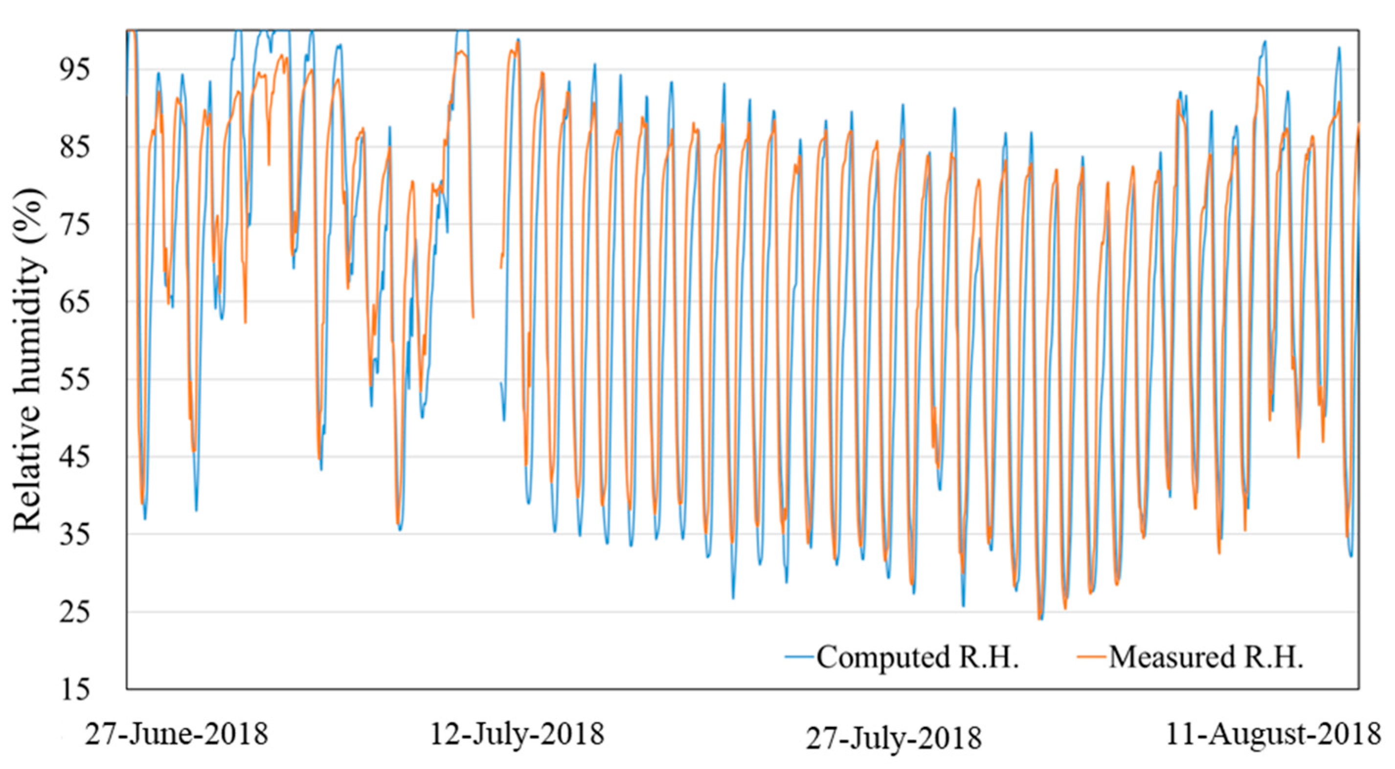
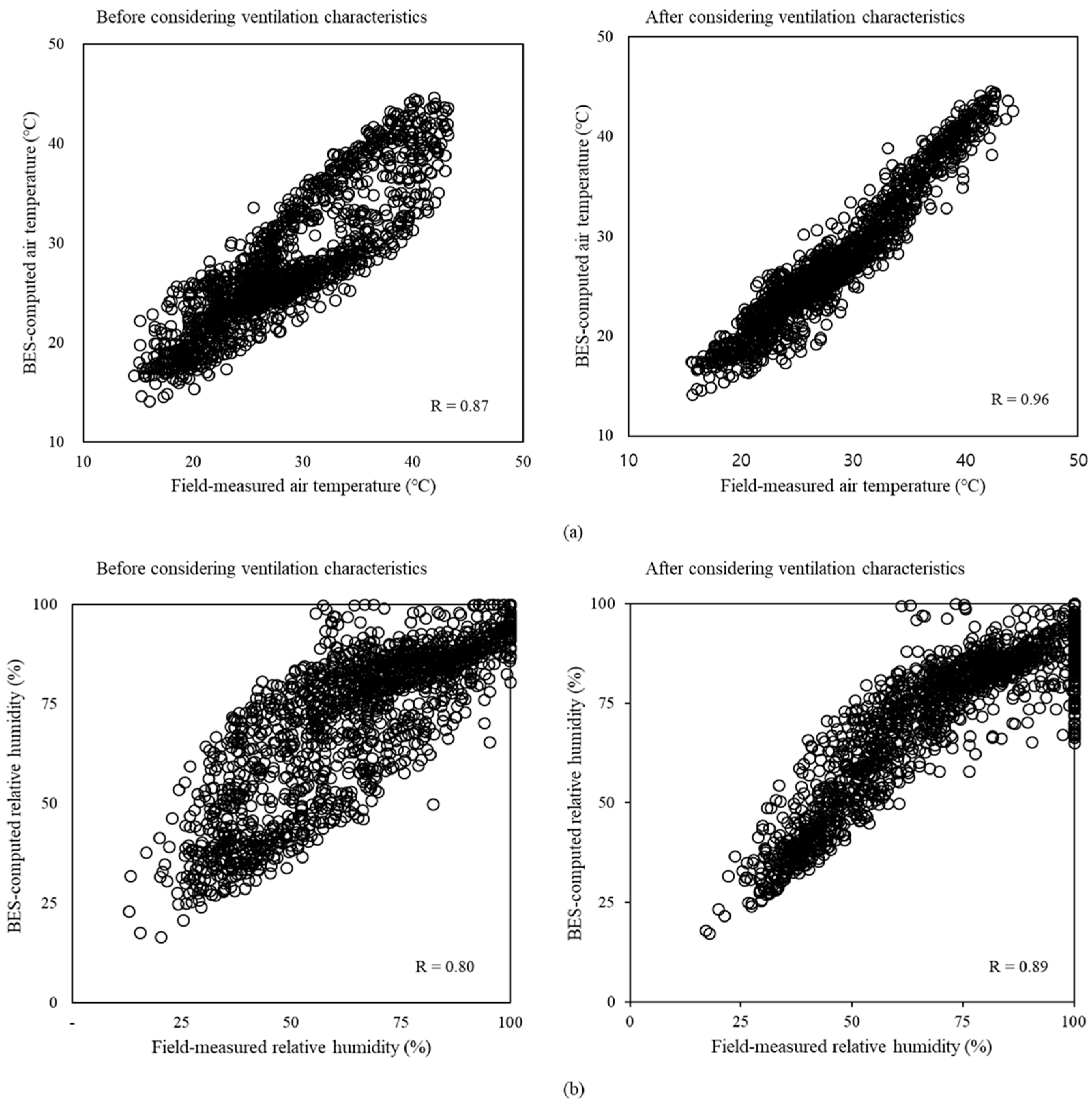
3.5. Design and Validation of a BES Model for Greenhouse

A greenhouse BES model, which can simulate thermal energy flow (conduction, radiation, convection) of the greenhouse according to external weather conditions and natural ventilation operation of the greenhouse, was designed using modules (components) to consider RAD, dew point temperature, and sky temperature provided by the TRNSYS simulation studio and experimental greenhouse model designed in TRNbuild (Figure 12). Figure 12 showed the module configuration of the greenhouse BES model considering the tomato energy exchange characteristics and the changes in weather, RAD, wet air, and dew point temperature for the target area. The crop energy exchange model was designed such that sensible and latent heat characteristics were considered in the greenhouse BES model from the multiple regression analysis between the microclimate environment inside the greenhouse, T_L, and ET. A calculator module was applied to the different relational expressions by dividing the growth stage of the tomato crop into seven stages. T_i and RH of the greenhouse according to the external weather conditions were computed using the final designed module-based BES model.

To validate the greenhouse BES model, T_i and RH data measured in the field experiment were compared with the computed results from the greenhouse BES model. Field-measured data measured in the experimental greenhouse at Andong University from 9 June 2018 to 15 August 2018 were used. The absolute error for T_i between the field-measured data and the BES-computed result of the greenhouse model was 2.77 °C (Figure 13), and the correlation coefficient was 0.87. In addition, the absolute error of RH was 11.1% (Figure 14) and the correlation coefficient was 0.80. It was considered that the accuracy of the greenhouse BES model could be reduced by applying a constant value to the ventilation rate, despite the changes in the external and internal weather environments over time in the process of designing the BES model. In other words, in the case of the greenhouse BES model, there was a limit in which it was not possible to quantitatively grasp the ventilation rate of invisible air in a naturally-ventilated greenhouse (NVG). Therefore, through an analysis of the wind environment around the experimental greenhouse, the ventilation rate (10.5 ACH) per hour predicted to occur in the greenhouse was applied. Because the energy load by ventilation computed from the greenhouse BES model was not considered according to the wind direction and speed around the greenhouse, it was found that the greenhouse BES model had a larger error than expected.

Figure 15 presented the results of the revalidation of the greenhouse BES model with the ventilation characteristics that occurred inside the greenhouse depending on the internal tomato crop (size) and external wind environment conditions. The BES-computed results of the greenhouse model considering the time-series ventilation rate were found to have an improved correlation with field-measured data than the conventional greenhouse BES model considering a fixed ACH for ventilation. Correlation is a method for analysing whether two independent variables have a linear relationship. If the ventilation characteristics that occur in a greenhouse were not taken into account, the correlation between the predicted T_i and actual T_i measured in the field experiment was 0.87. The correlation coefficient between the RH measured at the site and predicted RH was 0.80. However, the T_a and RH predicted by the greenhouse BES model considering real-time natural ventilation characteristics were considered to be better able to explain the trend compared to the previous greenhouse BES model, at 0.96 and 0.89, respectively (Figure 15). From this point, it was found that consideration of the change in ventilation rate according to the ambient wind environment was important in calculating the energy load of the greenhouse.

4. Conclusions

The crop model was designed by monitoring environmental variables (T_i, RH, RAD, T_L, and ET) that can be measured inside a greenhouse for a long time and analysing multiple regressions. The greenhouse BES model was designed considering the energy exchange characteristics of crops according to the changes in the microclimate environment inside the greenhouse. The designed greenhouse BES model was validated by comparing the field-measured data (T_i and RH) measured inside the greenhouse with the BES-computed results of the greenhouse model.

In this study, a greenhouse BES model was designed for energy load analysis by considering tomato crops inside a greenhouse using TRNSYS, a commercial software package. First, to consider the characteristics of the tomato energy exchange (sensible heat and latent heat) in the greenhouse BES model, a field experiment was conducted in a plastic greenhouse located at Andong University, and environmental variable data were continuously measured through field experiments.

A multiple regression model was designed using the measured environmental variable data, and a crop model was designed to consider the heat energy exchange characteristics of the sensible and latent heat of tomatoes. The accuracy of the tomato crop model for ET showed an error of 0.95 g plant⁻¹ h⁻¹. In addition, the error between the estimated T_L and field-measured T_L through the multiple regression model was 0.7 °C. The designed tomato crop model was applied to the greenhouse BES model for energy flow analysis into and out of the greenhouse by dividing tomato growth into seven stages. Finally, the designed greenhouse BES model was validated by comparing the field-measured data (T_i and RH) inside the greenhouse with the BES-computed results of the greenhouse model. The absolute error of T_i showed an average of 2.77 °C and 11.1% RH, and R² showed the accuracy of the model designed as 0.76 and 0.65, respectively.

To take into account the fluctuating ventilation characteristics over time, the CFD was used to evaluate the ventilation rate and discharge coefficients according to the greenhouse structure and internal crop characteristics. Depending on the conditions for scenario analysis, wind direction, wind speed, and tomato height inside the greenhouse, at least 5.4 ACH and up to 94.15 ACH occurred. Therefore, it was important to calculate the heat energy loss caused by ventilation in the simulation analysis for the energy load analysis of greenhouse, since it cannot simply assume a constant value.

When the greenhouse BES model was redesigned so that the changes in natural ventilation rates of the greenhouse over time were reflected in the greenhouse BES model, the average of the absolute error for T_i was 2.77 °C, and the current improved greenhouse BES model reduced the error by 1.2 °C. This resulted in an improvement of 42.6% accuracy. The average absolute error for RH was 7.7%, which reduced the error by 3.4% and improved the accuracy to 43.5%. In addition to the error, the correlation coefficient (R) of T_i and RH computed through the greenhouse BES model considering time-dependently changed natural ventilation characteristics were 0.96 and 0.89, respectively. It was found that the accuracy of the model for the trend could be improved using this new BES model compared to the previous greenhouse BES model.

References

1. Moon, J.; Shim, C.; Jung, O.; Hong, J.-W.; Han, J.; Song, Y.-I. Characteristics in Regional Climate Change over South Korea for Regional Climate Policy Measures: Based on Long-Term Observations. J. Clim. Chang. Res. 2020, 11, 755–770. [Google Scholar] [CrossRef]
2. Sethi, V.P.; Sumathy, K.; Lee, C.; Pal, D. Thermal modeling aspects of solar greenhouse microclimate control: A review on heating technologies. Sol. Energy 2013, 96, 56–82. [Google Scholar] [CrossRef]
3. De Zwart, H.F. Analyzing Energy-Saving Potentials in Greenhouse Cultivation Using a Simulation Model; University & Research Centre: Wageningen, The Netherlands, 1996. [Google Scholar]
4. Luo, W.; de Zwart, H.F.; DaiI, J.; Wang, X.; Stanghellini, C.; Bu, C. Simulation of Greenhouse Management in the Subtropics, Part I: Model Validation and Scenario Study for the Winter Season. Biosyst. Eng. 2005, 90, 307–318. [Google Scholar] [CrossRef]
5. Fabrizio, E. Energy reduction measures in agricultural greenhouses heating: Envelope, systems and solar energy collection. Energy Build. 2012, 53, 57–63. [Google Scholar] [CrossRef]
6. Joudi, K.A.; Farhan, A.A. A dynamic model and an experimental study for the internal air and soil temperatures in an innovative greenhouse. Energy Convers. Manag. 2015, 91, 76–82. [Google Scholar] [CrossRef]
7. Mohammadi, B.; Ranjbar, S.F.; Ajabshirchi, Y. Application of dynamic model to predict some inside environment variables in a semi-solar greenhouse. Inf. Process. Agric. 2018, 5, 279–288. [Google Scholar] [CrossRef]
8. Ahamed, M.S.; Guo, H.; Tanino, K. Modeling heating demands in a Chinese-style solar greenhouse using the transient building energy simulation model TRNSYS. J. Build. Eng. 2020, 29, 101114. [Google Scholar] [CrossRef]
9. Rasheed, A.; Kwak, C.S.; Kim, H.T.; Lee, H.W. Building Energy an Simulation Model for Analyzing Energy Saving Options of Multi-Span Greenhouses. Appl. Sci. 2020, 10, 6884. [Google Scholar] [CrossRef]
10. Chahidi, L.O.; Fossa, M.; Priarone, A.; Mechaqrane, A. Energy saving strategies in sustainable greenhouse cultivation in the mediterranean climate—A case study. Appl. Energy 2021, 282, 116156. [Google Scholar] [CrossRef]
11. Shin, H.; Kwak, Y.; Jo, S.-K.; Kim, S.-H.; Huh, J.-H. Applicability evaluation of a demand-controlled ventilation system in livestock. Comput. Electron. Agric. 2022, 196, 106907. [Google Scholar] [CrossRef]
12. Zhang, Y.; Gauthier, L.; de Halleux, D.; Dansereau, B.; Gosselin, A. Effect of covering materials on energy consumption and greenhouse microclimate. Agric. For. Meteorol. 1996, 82, 227–244. [Google Scholar] [CrossRef]
13. Boulard, T.; Wang, S. Greenhouse crop transpiration simulation from external climate conditions. Agric. For. Meteorol. 2000, 100, 25–34. [Google Scholar] [CrossRef]
14. Zhao, Y.; Teitel, M.; Barak, M. SE—Structures and Environment: Vertical Temperature and Humidity Gradients in a Naturally Ventilated Greenhouse. J. Agric. Eng. Res. 2001, 78, 431–436. [Google Scholar] [CrossRef]
15. Gupta, M.J.; Chandra, P. Effect of greenhouse design parameters on conservation of energy for greenhouse environmental control. Energy 2002, 27, 777–794. [Google Scholar] [CrossRef]
16. Luo, W.; Stanghellini, C.; Dai, J.; Wang, X.; de Zwart, H.F.; Bu, C. Simulation of Greenhouse Management in the Subtropics, Part II: Scenario Study for the Summer Season. Biosyst. Eng. 2005, 90, 433–441. [Google Scholar] [CrossRef]
17. Taki, M.; Ajabshirchi, Y.; Ranjbar, S.F.; Rohani, A.; Matloobi, M. Modeling and experimental validation of heat transfer and energy consumption in an innovative greenhouse structure. Inf. Process. Agric. 2016, 3, 157–174. [Google Scholar] [CrossRef] [Green Version]
18. Misra, D.; Ghosh, S. Microclimatic Modeling and Analysis of a Fog-Cooled Naturally Ventilated Greenhouse. Int. J. Environ. Agric. Biotechnol. 2017, 2, 997–1001. [Google Scholar] [CrossRef]
19. Rasheed, A.; Lee, J.W.; Lee, H.W. Development of a model to calculate the overall heat transfer coefficient of greenhouse covers. Span. J. Agric. Res. 2018, 15, e0208. [Google Scholar] [CrossRef] [Green Version]
20. Reyes-Rosas, A.; Molina-Aiz, F.D.; Valera, D.L.; López, A.; Khamkure, S. Development of a single energy balance model for prediction of temperatures inside a naturally ventilated greenhouse with polypropylene soil mulch. Comput. Electron. Agric. 2017, 142, 9–28. [Google Scholar] [CrossRef]
21. Ahamed, M.S.; Guo, H.; Tanino, K. Development of a thermal model for simulation of supplemental heating requirements in Chinese-style solar greenhouses. Comput. Electron. Agric. 2018, 150, 235–244. [Google Scholar] [CrossRef]
22. Singh, M.C.; Singh, J.P.; Singh, K.G. Development of a microclimate model for prediction of temperatures inside a naturally ventilated greenhouse under cucumber crop in soilless media. Comput. Electron. Agric. 2018, 154, 227–238. [Google Scholar] [CrossRef]
23. Mobtaker, H.G.; Ajabshirchi, Y.; Ranjbar, S.F.; Matloobi, M. Simulation of thermal performance of solar greenhouse in north-west of Iran: An experimental validation. Renew. Energy 2019, 135, 88–97. [Google Scholar] [CrossRef]
24. Semple, L.; Carriveau, R.; Ting, D. Assessing heating and cooling demands of closed greenhouse systems in a cold climate. Int. J. Energy Res. 2017, 41, 1903–1913. [Google Scholar] [CrossRef]
25. Shakir, S.M.; Farhan, A.A. Movable thermal screen for saving energy inside the greenhouse. Assoc. Arab. Univ. J. Eng. Sci. 2019, 26, 106–112. [Google Scholar] [CrossRef]
26. Lee, S.B.; Lee, I.B.; Homg, S.W.; Seo, I.H.; Bitog, P.J.; Kwon, K.S.; Ha, T.H.; Han, C.-P. Prediction of Greenhouse Energy Loads using Building Energy Simulation (BES). J. Korean Soc. Agric. Eng. 2012, 54, 113–124. [Google Scholar] [CrossRef]
27. Hassanien, R.H.E.; Li, M.; Lin, W.D. Advanced applications of solar energy in agricultural greenhouses. Renew. Sustain. Energy Rev. 2015, 54, 989–1001. [Google Scholar] [CrossRef]
28. Barichello, J.; Vesce, L.; Mariani, P.; Leonardi, E.; Braglia, R.; Di Carlo, A.; Canini, A.; Reale, A. Stable Semi-Transparent Dye-Sensitized Solar Modules and Panels for Greenhouse Application. Energies 2021, 14, 6393. [Google Scholar] [CrossRef]
29. Hamdi, I.; Kooli, S.; Elkhadraoui, A.; Azaizia, Z.; Abdelhamid, F.; Guizani, A. Experimental study and numerical modeling for drying grapes under solar greenhouse. Renew. Energy 2018, 127, 936–946. [Google Scholar] [CrossRef]
30. Thomas, Y.; Wang, L.; Denzer, A. Energy savings analysis of a greenhouse heated by waste heat. In Proceedings of the 15th IBPSA Conference, San Francisco, CA, USA, 7–9 August 2017; pp. 2512–2517. [Google Scholar]
31. Ha, T.; Lee, I.B.; Kwon, K.S.; Hong, S.W. Computation and field experiment validation of greenhouse energy load using Building Energy Simulation model. Int. J. Agric. Biol. Eng. 2015, 8, 116–127. [Google Scholar]
32. Lee, S.N. Design of a Greenhouse Energy Model Including Energy Exchange of Internal Plants and Its Application for Energy Loads Estimation. Master’s Dissertation, College of Agriculture and Life Sciences, Seoul National University, Seoul, Korea, 2017. [Google Scholar]
33. Lee, M.; Lee, I.-B.; Ha, T.-H.; Kim, R.-W.; Yeo, U.-H.; Lee, S.-Y.; Park, G.; Kim, J.-G. Estimation on Heating and Cooling Loads for a Multi-Span Greenhouse and Performance Analysis of PV System using Building Energy Simulation. Prot. Hortic. Plant Fact. 2017, 26, 258–267. [Google Scholar] [CrossRef]
34. Semple, L.; Carriveau, R.; Ting, D.S.K. A techno-economic analysis of seasonal thermal energy storage for greenhouse applications. Energy Build. 2017, 154, 175–187. [Google Scholar] [CrossRef]
35. Rasheed, A.; Lee, J.W.; Lee, H.W. Development and Optimization of a Building Energy Simulation Model to Study the Effect of Greenhouse Design Parameters. Energies 2018, 11, 2001. [Google Scholar] [CrossRef] [Green Version]
36. Alinejad, T.; Yaghoubi, M.; Vadiee, A. Thermo-environomic assessment of an integrated greenhouse with an adjustable solar photovoltaic blind system. Renew. Energy 2020, 156, 1–13. [Google Scholar] [CrossRef]
37. Cossu, M.; Murgia, L.; Ledda, L.; Deligios, P.A.; Sirigu, A.; Chessa, F.; Pazzona, A. Solar radiation distribution inside a greenhouse with south-oriented photovoltaic roofs and effects on crop productivity. Appl. Energy 2014, 133, 89–100. [Google Scholar] [CrossRef]
38. Marucci, A.; Zambon, I.; Colantoni, A.; Monarca, D. A combination of agricultural and energy purposes: Evaluation of a prototype of photovoltaic greenhouse tunnel. Renew. Sustain. Energy Rev. 2018, 82, 1178–1186. [Google Scholar] [CrossRef]
39. Shukla, A.; Tiwari, G.N.; Sodha, M. Thermal modeling for greenhouse heating by using thermal curtain and an earthair heat exchanger. Build. Environ. 2006, 41, 843–850. [Google Scholar] [CrossRef]
40. Cuce, E.; Harjunowibowo, D.; Cuce, P.M. Renewable and sustainable energy saving strategies for greenhouse systems: A comprehensive review. Renew. Sustain. Energy Rev. 2016, 64, 34–59. [Google Scholar] [CrossRef]
41. Chen, J.; Yang, J.; Zhao, J.; Xu, F.; Shen, Z.; Zhang, L. Energy demand forecasting of the greenhouses using nonlinear models based on model optimized prediction method. Neurocomputing 2016, 174, 1087–1100. [Google Scholar] [CrossRef]
42. Graamans, L.; van den Dobbelsteen, A.; Meinen, E.; Stanghellini, C. Plant factories; crop transpiration and energy balance. Agric. Syst. 2017, 153, 138–147. [Google Scholar] [CrossRef]
43. Majdoubi, H.; Boulard, T.; Fatnassi, H.; Senhaji, A.; Elbahi, S.; Demrati, H.; Mouqallid, M.; Bouirden, L. Canary Greenhouse CFD Nocturnal Climate Simulation. Open J. Fluid Dyn. 2016, 6, 88–100. [Google Scholar] [CrossRef] [Green Version]
44. Talbot, M.-H.; Monfet, D. Estimating the impact of crops on peak loads of a Building-Integrated Agriculture space. Sci. Technol. Built Environ. 2020, 26, 1448–1460. [Google Scholar] [CrossRef]
45. Li, B.; Shi, B.J.; Yao, Z.Z.; Shukla, M.K.; Du, T.S. Energy partitioning and microclimate of solar greenhouse under drip and furrow irrigation systems. Agric. Water Manag. 2020, 234, 106096. [Google Scholar] [CrossRef]
46. Boulard, T.; Baille, A. Analysis of thermal performance of a greenhouse as a solar collector. Energy Agric. 1987, 6, 17–26. [Google Scholar] [CrossRef]
47. Eumorfopoulou, E.; Aravantinos, D. The contribution of a planted roof to the thermal protection of buildings in Greece. Energy Build. 1998, 27, 29–36. [Google Scholar] [CrossRef]
48. Henshaw, P. Modelling changes to an unheated greenhouse in the Canadian subarctic to lengthen the growing season. Sustain. Energy Technol. Assess. 2017, 24, 31–38. [Google Scholar] [CrossRef]
49. Attar, I.; Naili, N.; Khalifa, N.; Hazami, M.; Farhat, A. Parametric and numerical study of a solar system for heating a greenhouse equipped with a buried exchanger. Energy Convers. Manag. 2013, 70, 163–173. [Google Scholar] [CrossRef]
50. Zhang, L.; Xu, P.; Mao, J.; Tang, X.; Li, Z.; Shi, J. A low cost seasonal solar soil heat storage system for greenhouse heating: Design and pilot study. Appl. Energy 2015, 156, 213–222. [Google Scholar] [CrossRef]
51. Vadiee, A.; Martin, V. Energy analysis and thermoeconomic assessment of the closed greenhouse—The largest commercial solar building. Appl. Energy 2013, 102, 1256–1266. [Google Scholar] [CrossRef]
52. Bournet, P.-E.; Boulard, T. Effect of ventilator configuration on the distributed climate of greenhouses: A review of experimental and CFD studies. Comput. Electron. Agric. 2010, 74, 195–217. [Google Scholar] [CrossRef]
53. Piscia, D.; Montero, J.I.; Baeza, E.; Bailey, B.J. A CFD greenhouse night-time condensation model. Biosyst. Eng. 2012, 111, 141–154. [Google Scholar] [CrossRef]
54. Bartzanas, T.; Kacira, M.; Zhu, H.; Karmakar, S.; Tamimi, E.; Katsoulas, N.; In BokLeef, C.; Kittas, C. Computational fluid dynamics applications to improve crop production systems. Comput. Electron. Agric. 2013, 93, 151–167. [Google Scholar] [CrossRef]
55. Boulard, T.; Roy, J.C.; Pouillard, J.B.; Fatnassi, H.; Grisey, A. Modelling of micrometeorology, canopy transpiration and photosynthesis in a closed greenhouse using computational fluid dynamics. Biosyst. Eng. 2017, 158, 110–133. [Google Scholar] [CrossRef]
56. Kim, M.-H.; Lee, D.-W.; Yun, R.; Heo, J. Operational Energy Saving Potential of Thermal Effluent Source Heat Pump System for Greenhouse Heating in Jeju. Int. J. Air-Cond. Refrig. 2017, 25, 1750030. [Google Scholar] [CrossRef]
57. Lee, S.-Y.; Lee, I.-B.; Kim, R.-W. Evaluation of wind-driven natural ventilation of single-span greenhouses built on reclaimed coastal land. Biosyst. Eng. 2018, 171, 120–142. [Google Scholar] [CrossRef]
58. Klein, S.A. TRNSYS 18: A Transient System Simulation Program, Solar Energy Laboratory, University of Wisconsin, Madison, WI, USA. 2017. Available online: https://sel.me.wisc.edu/trnsys (accessed on 3 September 2020).
59. Fatnassi, H.; Boulard, T.; Poncet, C.; Katsoulas, N.; Bartzanas, T.; Kacira, M.; Giday, H.; Lee, I.B. Computational fluid dynamics modelling of the microclimate within the boundary layer of leaves leading to improved pest control management and low-input greenhouse. Sustainability 2021, 13, 8310. [Google Scholar] [CrossRef]
60. Yeo, U.H.; Lee, I.B.; Kim, R.W.; Lee, S.Y.; Kim, J.G. Computational fluid dynamics evaluation of pig house ventilation systems for improving the internal rearing environment. Biosyst. Eng. 2019, 186, 259–278. [Google Scholar] [CrossRef]
61. Kim, R.W.; Kim, J.G.; Lee, I.B.; Yeo, U.H.; Lee, S.Y.; Decano-Valentin, C. Development of three-dimensional visualisation technology of the aerodynamic environment in a greenhouse using CFD and VR technology, part 1: Development of VR a database using CFD. Biosyst. Eng. 2021, 207, 33–58. [Google Scholar] [CrossRef]
62. Lee, S.Y.; Kim, J.G.; Kim, R.W.; Yeo, U.H.; Lee, I.B. Development of three-dimensional visualisation technology of aerodynamic environment in fattening pig house using CFD and VR technology. Comput. Electron. Agric. 2022, 194, 106709. [Google Scholar] [CrossRef]
63. Teitel, M.; Ozer, S.; Mendelovich, V. Airflow temperature and humidity patterns in a screenhouse with a flat insect-proof screen roof and impermeable sloping walls–Computational fluid dynamics (CFD) results. Biosyst. Eng. 2022, 214, 165–176. [Google Scholar] [CrossRef]
64. Norton, T.; Sun, D.-W.; Grant, J.; Fallon, R.; Dodd, V. Applications of computational fluid dynamics (CFD) in the modelling and design of ventilation systems in the agricultural industry: A review. Bioresour. Technol. 2007, 98, 2386–2414. [Google Scholar] [CrossRef]
65. Monteith, J.L.; Unsworth, M.H. Principles of Environmental Physics; Edward Arnold: London, UK, 1990. [Google Scholar]
66. Ortega-Farias, S.O.; Olioso, A.; Fuentes, S.; Valdes, H. Latent heat flux over a furrow-irrigated tomato crop using Penman–Monteith equation with a variable surface canopy resistance. Agric. Water Manag. 2006, 82, 421–432. [Google Scholar] [CrossRef]
67. Kim, R.W.; Lee, I.B.; Kwon, K.S. Evaluation of wind pressure acting on multi-span greenhouses using CFD technique, Part 1: Development of the CFD model. Biosyst. Eng. 2017, 164, 235–256. [Google Scholar] [CrossRef]
68. Richards, P.J. Computational Modelling of Wind Flow around Low-Rise Buildings Using PHOENICS; AFRC Institute of Engineering Research Wrest Park, Silsoe Research Institute, University of Reading: Bedfordshire, UK, 1989. [Google Scholar]
69. Lee, I.-B.; Sase, S.; Sung, S.-H. Evaluation of CFD Accuracy for the Ventilation Study of a Naturally Ventilated Broiler House. Jpn. Agric. Res. Q. JARQ 2007, 41, 53–64. [Google Scholar] [CrossRef] [Green Version]
70. Bartzanas, T.; Kittas, C.; Sapounas, A.; Nikita-Martzopoulou, C. Analysis of airflow through experimental rural buildings: Sensitivity to turbulence models. Biosyst. Eng. 2007, 97, 229–239. [Google Scholar] [CrossRef]
71. Lee, I.B.; Yun, N.K.; Boulard, T.; Roy, J.C.; Lee, S.H.; Kim, G.W.; Lee, S.; Kwon, S.H. Development of an aerodynamic simulation for studying microclimate of plant canopy in greenhouse-(1) Study on aerodynamic resistance of tomato canopy through wind tunnel experiment. J. Bio-Environ. Control 2006, 15, 289–295. [Google Scholar]
72. Lee, I.B.; Yun, N.K.; Boulard, T.; Roy, J.C.; Lee, S.H.; Kim, G.W.; Hong, S.-W.; Sung, S.H. Development of an aerodynamic simulation for studying microclimate of plant canopy in greenhouse-(2) Development of CFD model to study the effect of tomato plants on internal climate of greenhouse. J. Bio-Environ. Control 2006, 15, 296–305. [Google Scholar]
73. Kittas, C.; Boulard, T.; Papadakis, G. Natural ventilation of a greenhouse with ridge and side openings: Sensitivity to temperature and wind effects. Trans. ASAE 1997, 40, 415–425. [Google Scholar] [CrossRef]
74. Sawachi, T.; Ken-Ichi, N.; Kiyota, N.; Seto, H.; Nishizawa, S.; Ishikawa, Y. Wind Pressure and Air Flow in a Full-Scale Building Model under cross Ventilation. Int. J. Vent. 2004, 2, 343–357. [Google Scholar] [CrossRef]
75. Sethi, V.P. On the selection of shape and orientation of a greenhouse: Thermal modeling and experimental validation. Sol. Energy 2009, 83, 21–38. [Google Scholar] [CrossRef]
76. Ntinas, G.K.; Fragos, V.P.; Nikita-Martzopoulou, C. Thermal analysis of a hybrid solar energy saving system inside a greenhouse. Energy Convers. Manag. 2014, 81, 428–439. [Google Scholar] [CrossRef]
77. Chen, J.; Xu, F.; Tan, D.-P.; Shen, Z.; Zhang, L.; Ai, Q. A control method for agricultural greenhouses heating based on computational fluid dynamics and energy prediction model. Appl. Energy 2015, 141, 106–118. [Google Scholar] [CrossRef]
78. Mashonjowa, E.; Ronsse, F.; Milford, J.R.; Pieters, J.G. Modelling the thermal performance of a naturally ventilated greenhouse in Zimbabwe using a dynamic greenhouse climate model. Sol. Energy 2013, 91, 381–393. [Google Scholar] [CrossRef]
79. Lee, H.W.; Sim, S.Y.; Kim, Y.S. Characteristics of PPF Transmittance and Heat Flow by Double Covering Methods of Plastic Film in Tomato Greenhouse. J. Korean Soc. Agric. Eng. 2010, 52, 11–18. [Google Scholar] [CrossRef] [Green Version]
80. Monte, J.A.; De Carvalho, D.F.; Medici, L.O.; da Silva, L.D.B.; Pimentel, C. Growth analysis and yield of tomato crop under different irrigation depths. Rev. Bras. De Eng. Agrícola E Ambient. 2013, 17, 926–931. [Google Scholar] [CrossRef] [Green Version]
81. Albright, L.D. Environment Control for Animals and Plants; American Society of Agricultural Engineers: St. Joseph, MI, USA, 1990. [Google Scholar]
82. Lindley, J.A.; Whitaker, J.H. Agricultural Buildings and Structures; ASAE: St. Joseph, MI, USA, 1996. [Google Scholar]
83. Karava, P.; Stathopoulos, T.; Athienitis, A.K. Wind-induced natural ventilation analysis. Sol. Energy 2007, 81, 20–30. [Google Scholar] [CrossRef]
84. Chu, C.R.; Chiu, Y.H.; Chen, Y.J.; Wang, Y.W.; Chou, C.P. Turbulence effects on the discharge coefficient and mean flow rate of wind-driven cross-ventilation. Build. Environ. 2009, 44, 2064–2072. [Google Scholar] [CrossRef]
85. Kurabuchi, T.; Ohba, M.; Endo, T.; Akamine, Y.; Nakayama, F. Local Dynamic Similarity Model of Cross-Ventilation Part 1—Theoretical Framework. Int. J. Vent. 2004, 2, 371–382. [Google Scholar] [CrossRef]
86. Ohba, M.; Kurabuchi, T.; Tomoyuki, E.; Akamine, Y.; Kamata, M.; Kurahashi, A. Local Dynamic Similarity Model of Cross-Ventilation Part 2—Application of Local Dynamic Similarity Model. Int. J. Vent. 2004, 2, 383–394. [Google Scholar] [CrossRef]
87. Carey, P.S.; Etheridge, D.W. Direct wind tunnel modelling of natural ventilation for design purposes. Build. Serv. Eng. Res. Technol. 1999, 20, 131–142. [Google Scholar] [CrossRef]
88. Vickery, B.J.; Karakatsanis, C. External wind pressure distributions and induced internal ventilation flow in low-rise industrial and domestic structures. ASHRAE Trans. 1987, 93, 2198–2213. [Google Scholar]
Figure 1. Research flow for analysing the thermal energy load of the experimental greenhouse.
Agriculture 12 00903 g001
Figure 2. Experimental greenhouse in Andong University in Korea: (a) outside the greenhouse, (b) inside the greenhouse, and (c) three-dimensional configuration (latitude: 36°54′ N, longitude: 128°80′ E).
Agriculture 12 00903 g002
Figure 3. Environmental variables for monitoring the microclimate inside and outside the experimental greenhouse, and sensor installation location for each environmental variable.
Agriculture 12 00903 g003
Figure 4. Schematic diagram of self-manufactured system time-dependently measuring ET of tomato crops inside the greenhouse.
Agriculture 12 00903 g004
Figure 5. A monitoring device for the amount of evaporation used in greenhouses: (a) design process and (b) growing tomatoes.
Agriculture 12 00903 g005
Figure 6. Designed CFD model for greenhouse and computational domain: (a) top view and (b) side view for CFD computation domain.
Agriculture 12 00903 g006
Figure 7. Definition of wind direction based on the experimental building.
Agriculture 12 00903 g007
Figure 8. Change of tomato LAI measured through the destruction investigation (circle: measured LAI and dotted line: changing trend).
Agriculture 12 00903 g008
Figure 9. Airflow pattern inside and outside the greenhouse according to the WD: (a) 0° and (b) 90°.
Agriculture 12 00903 g009
Figure 10. Airflow pattern inside and outside the greenhouse according to the WD of 45° (WS: 3.0 m s−1, and crop height: 1.0 m).
Agriculture 12 00903 g010
Figure 11. Distribution of the WS of the greenhouse (side view) (a) without tomatoes and (b) with tomatoes (WS: 3.0 m s−1, WD: 90°, and crop height: 1.0 m).
Agriculture 12 00903 g011
Figure 12. Module configuration of greenhouse BES model to consider tomato model (sensible and latent heat) by growth stage.
Agriculture 12 00903 g012
Figure 13. Validation between BES-computed and field-measured air temperatures (°C).
Agriculture 12 00903 g013
Figure 14. Validation between BES-computed and field-measured relative humidity (%).
Agriculture 12 00903 g014
Figure 15. Comparison between BES-computed result of the greenhouse model and field-measured data considering ventilation characteristics of the greenhouse (a) air temperature and (b) relative humidity.
Agriculture 12 00903 g015