
Optimization of Voltage Security with Placement of FACTS Device Using Modified Newton–Raphson Approach: A Case Study of Nigerian Transmission Network


Abstract
1. Introduction
2. Materials and Methods
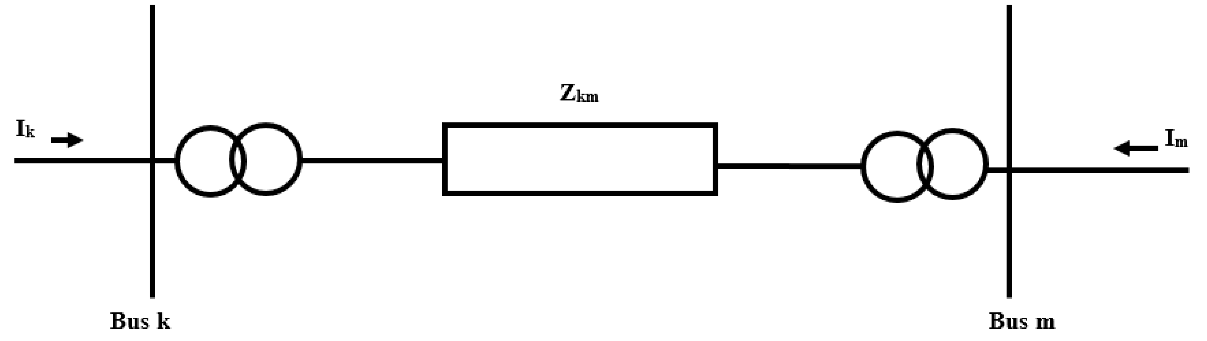
2.1. Newton–Raphson Power Flow Method
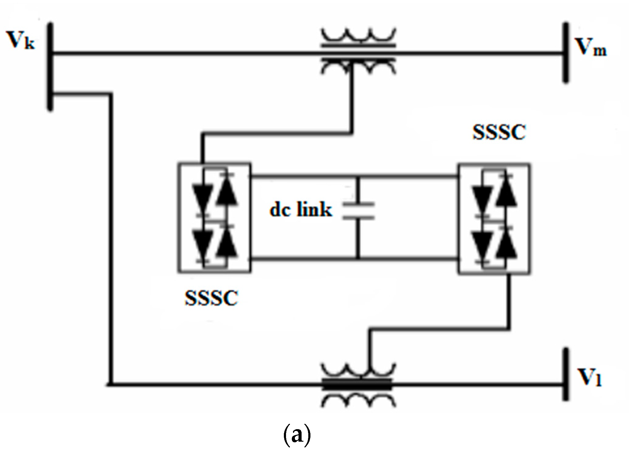
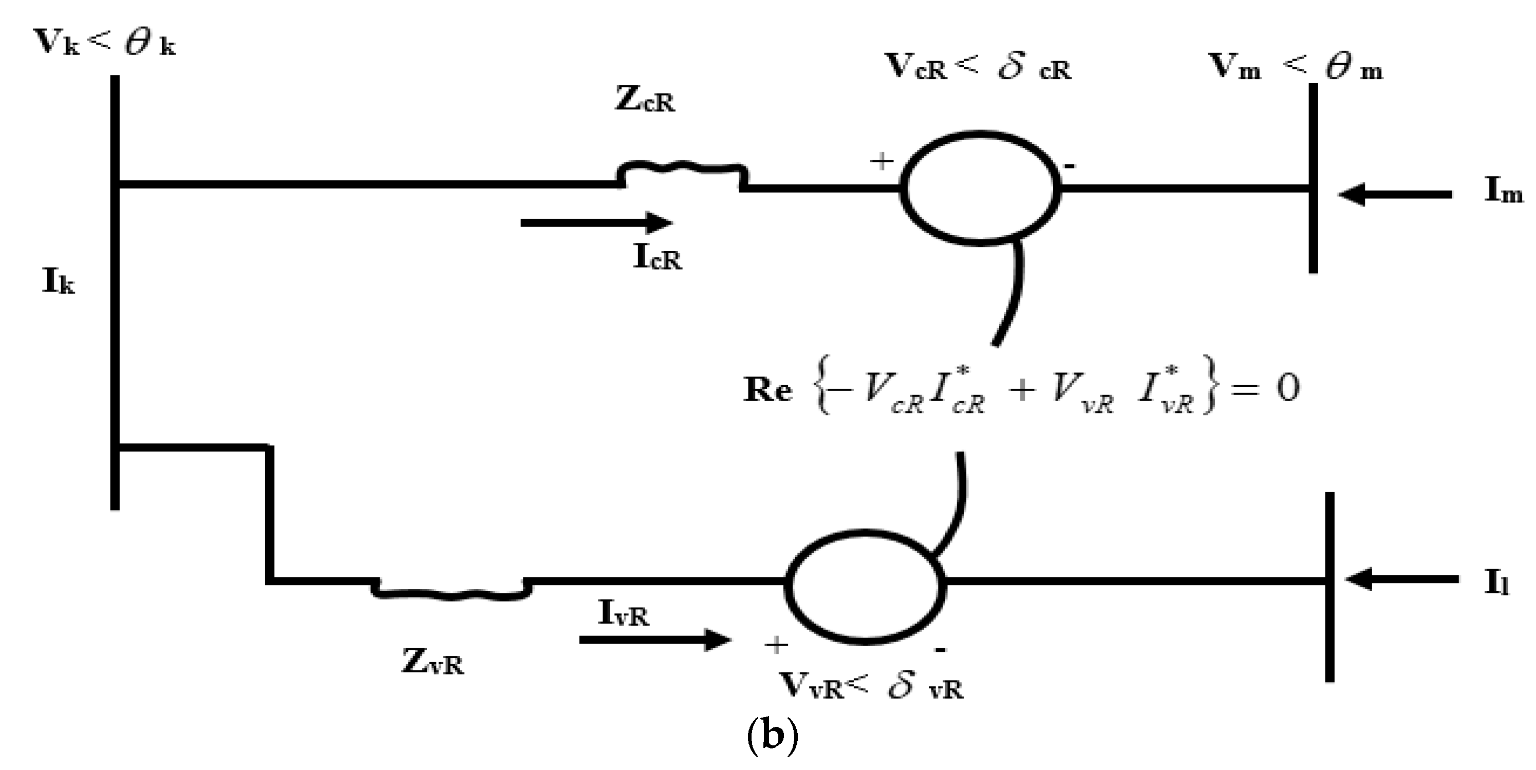
2.2. Power Flow Model of an IPFC
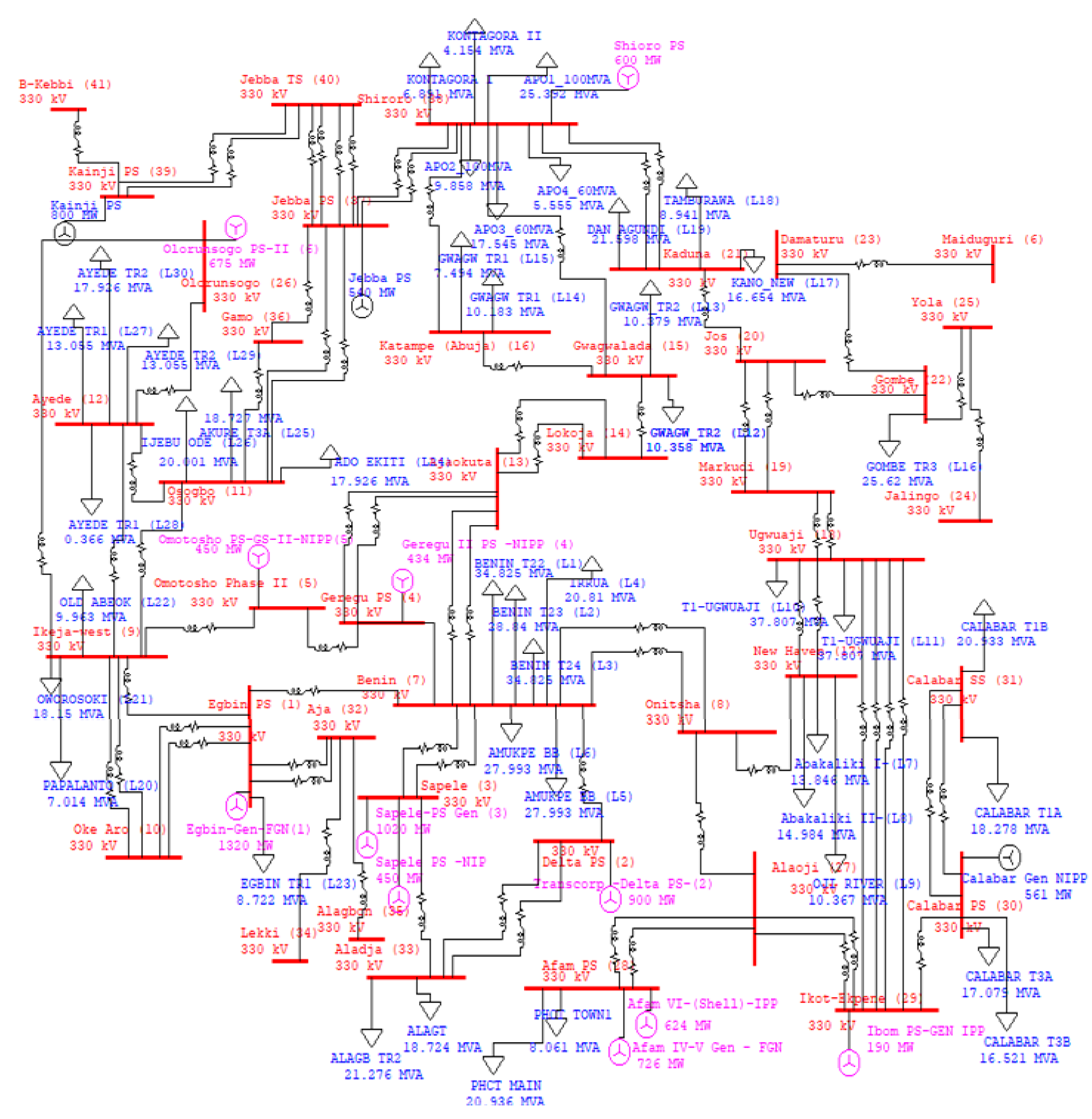
2.3. Case Study
3. Results
4. Discussion
5. Conclusions
Author Contributions
Funding
Institutional Review Board Statement
Informed Consent Statement
Data Availability Statement
Conflicts of Interest
Abbreviations
| DA | Differential evolution |
| DFC | Dynamic flow controller |
| FA | Firefly algorithms |
| FACTS | Flexible AC transmission system |
| GSA | Gravitational search algorithm |
| GUPFC | General unified power flow controller |
| IPFC | Interline power flow controller |
| PSO | Particle swam optimization |
| SVC | Static var compensator |
| SSSC | Static synchronous series compensator |
| STATCOM | Static synchronous compensator |
| TCSC | Thyristor controlled series compensator |
| UPFC | Unified power flow controller |
| Symbols | |
| S | Complex power injection |
| P | Active power injection |
| Q | Reactive power injection |
| I | Injected current |
| Y | Line admittance |
| G | line conductance |
| B | Line susceptance |
| r | Number of iterative step |
| Z | line impedance |
| Pcalc | Active power calculated |
| Pspec | Active power specified |
| Pload | Active power consume |
| Pgen | Active power generated |
| Qcalc | Reactive power calculated |
| Qspec | Reactive power specified |
| Qload | Reactive power consume |
| Qgen | Reactive power consume |
| Converter 1 phase angle | |
| Converter 2 phase angle | |
| ϴ | Bus angle |
| Subscript | |
| k, m, L | Buses |
| cR | Converter 1 |
| vR | Converter 2 |
| km | Line linking bus k to bus m |
| kL | Line linking bus k to bus L |
References
- Ghiasi, M. Technical and economic evaluation of power quality performance using FACTS devices considering renewable micro-grids. Renew. Energy Focus 2019, 29, 49–62. [Google Scholar] [CrossRef]
- Steele, A.J.H.; Burnett, J.W.; Bergstrom, J.C. The impact of variable renewable energy resources on power system reliability. Energy Policy 2021, 151, 111947. [Google Scholar] [CrossRef]
- Aljohani, T.M.; Beshir, M.J. Distribution System Reliability Analysis for Smart Grid Applications. Smart Grid Renew. Energy 2017, 8, 240–251. [Google Scholar] [CrossRef]
- Ewaoche, O.J.; Nwulu, N. Design and Simulation of UPFC and IPFC for Voltage Stability Uder a Single Line Contingency: A Comparative Study. In Proceedings of the International Conference on Industrial Engineering and Operations Management, Washington, DC, USA, 27–29 September 2018. [Google Scholar]
- Hingorani, N.G.; Gyugyi, L. Understanding FACTS: Concepts and Technology of Flexible AC Transmission Systems; IEEE Press: New York, NY, USA, 2000; Volume 148. [Google Scholar]
- Mutegi, M.A.; Nnamdi, N.I. Optimal Placement of FACTS Devices Using Filter Feeding Allogenic Engineering Algorithm. Technol. Econ. Smart Grids Sustain. Energy 2022, 7, 1–18. [Google Scholar] [CrossRef]
- Singh, S.; Jaiswal, S.P. Enhancement of ATC of micro grid by optimal placement of TCSC. Mater. Today Proc. 2019, 34, 787–792. [Google Scholar] [CrossRef]
- Ersavas, C.; Karatepe, E. Optimum allocation of FACTS devices under load uncertainty based on penalty functions with genetic algorithm. Electr. Eng. 2017, 99, 73–84. [Google Scholar] [CrossRef]
- Khan, I.; Mallick, M.A.; Rafi, M.; Mirza, M.S. Optimal placement of FACTS controller scheme for enhancement of power system security in Indian scenario. J. Electr. Syst. Inf. Technol. 2015, 2, 161–171. [Google Scholar] [CrossRef]
- Hagh, M.T.; Alipour, M.; Teimourzadeh, S. Application of HGSO to security based optimal placement and parameter setting of UPFC. Energy Convers. Manag. 2014, 86, 873–885. [Google Scholar] [CrossRef]
- Kang, T.; Yao, J.; Duong, T.; Yang, S.; Zhu, X. A hybrid approach for power system security enhancement via optimal installation of flexible ac transmission system (FACTS) devices. Energies 2017, 10, 1305. [Google Scholar] [CrossRef]
- Ewaoche, O.J.; Nwulu, N. Fault Clearance and Transmission System Stability Enhancement using Unified Power Flow Controller. In Proceedings of the International Conference on Computational Techniques, Electronics and Mechanical Systems (CTEMS), Belgaum, India, 21–22 December 2018; pp. 86–91. [Google Scholar] [CrossRef]
- Lund, A.A.; Keerio, M.U.; Koondhar, M.A.; Jamali, M.I.; Tunio, A.Q. Investigation of advanced control for unified power flow controller (UPFC) to improve the performance of power system. J. Appl. Emerg. Sci. 2021, 11, 67. [Google Scholar] [CrossRef]
- Magaji, N.; Mustafa, M.W. Optimal location and signal selection of UPFC device for damping oscillation. Int. J. Electr. Power Energy Syst. 2011, 33, 1031–1042. [Google Scholar] [CrossRef]
- Mahdad, B.; Srairi, K. Application of a combined superconducting fault current limiter and STATCOM to enhancement of power system transient stability. Phys. C Supercond. Appl. 2013, 495, 160–168. [Google Scholar] [CrossRef]
- Sode-Yome, A.; Mithulananthan, N.; Lee, K.Y. Reactive Power Loss Sensitivity Approach in Placing FACTS Devices and UPFC; IFAC: New York, NY, USA, 2012; Volume 8. [Google Scholar]
- Bakir, H.; Kulaksiz, A.A. Modelling and voltage control of the solar-wind hybrid micro-grid with optimized STATCOM using GA and BFA. Eng. Sci. Technol. Int. J. 2020, 23, 576–584. [Google Scholar] [CrossRef]
- Singh, B.; Agrawal, G. Enhancement of voltage profile by incorporation of SVC in power system networks by using optimal load flow method in MATLAB/Simulink environments. Energy Rep. 2018, 4, 418–434. [Google Scholar] [CrossRef]
- Ewaoche, O.J.; Nwulu, N. Modelling and Simulation of Interline Power Flow Controller for Improved Transmission System Security. In Proceedings of the International Conference on Computational Techniques, Electronics and Mechanical Systems (CTEMS), Belgaum, India, 21–22 December 2018; pp. 250–255. [Google Scholar] [CrossRef]
- Seifi, A.; Gholami, S.; Shabanpour, A. Power Flow Study and Comparison of FACTS: Series (SSSC), Shunt (STATCOM), and Shunt-Series (UPFC). Pac. J. Sci. Technol. 2010, 11, 129–137. [Google Scholar]
- Li, S.; Wang, T.; Zhang, H.; Wang, L.; Jiang, Y.; Xue, J. Sensitivity-based coordination to controllable ranges of UPFCs to avoid active power loop flows. Int. J. Electr. Power Energy Syst. 2020, 114, 105383. [Google Scholar] [CrossRef]
- Mishra, A.; Gundavarapu, V.N.K. Contingency management of power system with Interline Power Flow Controller using Real Power Performance Index and Line Stability Index. Ain Shams Eng. J. 2016, 7, 209–222. [Google Scholar] [CrossRef]
- Aghaei, J.; Gitizadeh, M.; Kaji, M. Placement and operation strategy of FACTS devices using optimal continuous power flow. Sci. Iran. 2012, 19, 1683–1690. [Google Scholar] [CrossRef][Green Version]
- Barrios-Martínez, E.; Ángeles-Camacho, C. Technical comparison of FACTS controllers in parallel connection. J. Appl. Res. Technol. 2017, 15, 36–44. [Google Scholar] [CrossRef]
- Jamnani, J.G.; Pandya, M. Coordination of SVC and TCSC for management of power flow by particle swarm optimization. Energy Procedia 2019, 156, 321–326. [Google Scholar] [CrossRef]
- Taher, S.A.; Amooshahi, M.K. New approach for optimal UPFC placement using hybrid immune algorithm in electric power systems. Int. J. Electr. Power Energy Syst. 2012, 43, 899–909. [Google Scholar] [CrossRef]
- Sahu, P.R.; Hota, P.K.; Panda, S. Power system stability enhancement by fractional order multi input SSSC based controller employing whale optimization algorithm. J. Electr. Syst. Inf. Technol. 2018, 5, 326–336. [Google Scholar] [CrossRef]
- Inkollu, S.R.; Kota, V.R. Optimal setting of FACTS devices for voltage stability improvement using PSO adaptive GSA hybrid algorithm. Eng. Sci. Technol. Int. J. 2016, 19, 1166–1176. [Google Scholar] [CrossRef]
- Mishra, A.; Kumar, G.V.N. Congestion management of deregulated power systems by optimal setting of Interline Power Flow Controller using Gravitational Search algorithm. J. Electr. Syst. Inf. Technol. 2017, 4, 198–212. [Google Scholar] [CrossRef]
- Amarendra, A.; Srinivas, L.R.; Rao, R.S. Identification of the best location and size of IPFC to optimize the cost and to improve the power system security using Firefly optimization algorithm. Mater. Today Proc. 2020. [Google Scholar] [CrossRef]
- Gbadamosi, S.L.; Nwulu, N.I. A multi-period composite generation and transmission expansion planning model incorporating renewable energy sources and demand response. Sustain. Energy Technol. Assess. 2020, 39, 100726. [Google Scholar] [CrossRef]
- Acha, E.; Fuerte-Esquivel, H.; Ambriz-Perez, C.R.; Cesar, A.-C. FACTS Modelling and Simulation in Power Networks; The Atrium, Southern Gate, Chichester, West Sussex PO19 8SQ; John Wiley & Sons Ltd: Hoboken, NJ, USA, 2004; Volume 148. [Google Scholar]
- Babu, A.V.N.; Sivanagaraju, S. Mathematical modelling, analysis and effects of interline power flow controller (IPFC) parameters in power flow studies. In Proceedings of the India International Conference on Power Electronics 2010 (IICPE2010), New Delhi, India, 28–30 January 2011. [Google Scholar] [CrossRef]
- Karami, A.; Rashidinejad, M.; Gharaveisi, A.A. Voltage Security Enhancement And Congestion Management Via Statcom & Ipfc Using Artificial Intelligence. Iran. J. Sci. Technol. Trans. B Eng. 2007, 31, 289–301. [Google Scholar]
- Okampo, E.J.; Nwulu, N.; Bokoro, P.N. Transient stability analysis of a transmission network using eigenvalue principles with automated var compensation: A case study of the nigerian eastern grid. Energies 2021, 14, 5289. [Google Scholar] [CrossRef]


| Buses | 41 |
| Lines | 77 |
| Generators | 13 |
| Loads | 17 |
| Power rate (MVA) | 100 |
| From Bus | To Bus | Line | P Flow | Q Flow | P Loss | Q Loss |
|---|---|---|---|---|---|---|
| [p.u.] | [p.u.] | [p.u.] | [p.u.] | |||
| AfamPS(46) | Aja(39) | 1 | 0.780641 | −0.7207 | 0.006116 | −1.26177 |
| Aja(39) | Ajaokuta(17) | 2 | −1.01058 | −12.5873 | 0.418722 | 3.110249 |
| Aja(39) | Ajaokuta(17) | 3 | −1.01058 | −12.5873 | 0.418722 | 3.110249 |
| Ajaokuta(17) | Akangba(34) | 4 | 2.900855 | −1.96867 | 0.046359 | −1.38056 |
| Ajaokuta(17) | Akangba(34) | 5 | 2.900855 | −1.96867 | 0.046359 | −1.38056 |
| Ajaokuta(17) | Aladja(40) | 6 | −3.38736 | −0.46289 | 0.035998 | −0.80328 |
| Ajaokuta(17) | Aladja(40) | 7 | −3.38736 | −0.46289 | 0.035998 | −0.80328 |
| Ajaokuta(17) | Aladja(40) | 8 | −3.38736 | −0.46289 | 0.035998 | −0.80328 |
| Alagbon(45) | Ajaokuta(17) | 9 | −1.09211 | −1.11017 | 0.000387 | −0.05245 |
| Alagbon(45) | Ajaokuta(17) | 10 | −1.09211 | −1.11017 | 0.000387 | −0.05245 |
| Akangba(34) | Alaoji(42) | 11 | 1.242819 | 10.45204 | 0.335718 | 2.000311 |
| Akangba(34) | Alaoji(42) | 12 | 1.242819 | 10.45204 | 0.335718 | 2.000311 |
| Akangba(34) | Ayede(23) | 13 | 2.294793 | 0.188437 | 0.009949 | −0.63041 |
| Akangba(34) | Ayede(23) | 14 | 2.294793 | 0.188437 | 0.009949 | −0.63041 |
| Aladja(40) | Ganmo(22) | 15 | −0.41409 | −2.83588 | 0.018841 | −1.79585 |
| Aladja(40) | Ganmo(22) | 16 | −0.41409 | −2.83588 | 0.018841 | −1.79585 |
| Aladja(40) | Ganmo(22) | 17 | −0.41409 | −2.83588 | 0.018841 | −1.79585 |
| Aladja(40) | Ikot-Ekpene(48) | 18 | −2.1721 | 4.906201 | 0.186024 | 0.145485 |
| Aladja(40) | Lokoja(15) | 19 | −6.82618 | 8.505772 | 0.283937 | 1.700441 |
| Ayede(23) | B-Kebbi(1) | 20 | 2.936046 | −0.52279 | 0.030969 | −1.12041 |
| Ayede(23) | Benin(30) | 21 | −0.43084 | 0.732819 | 0.008588 | −1.31713 |
| Ayede(23) | Benin(30) | 22 | −0.43084 | 0.732819 | 0.008588 | −1.31713 |
| Ayede(23) | Benin(30) | 23 | −0.43084 | 0.732819 | 0.008588 | −1.31713 |
| Benin(30) | CalabarPS(47) | 24 | −0.25334 | 8.836865 | 0.511145 | 3.229433 |
| Benin(30) | NewHaven(32) | 25 | −2.17614 | −1.59881 | 0.02676 | −1.51277 |
| Benin(30) | NewHaven(32) | 26 | −2.17614 | −1.59881 | 0.02676 | −1.51277 |
| CalabarSS(37) | CalabarPS(47) | 27 | 6.33 × 10⁻¹¹ | −9.8 × 10⁻¹² | 0.001442 | −0.56042 |
| Damaturu(3) | Ikot-Ekpene(48) | 28 | 4.12323 | −1.19477 | 0.079501 | 0.129835 |
| DeltaPS(41) | CalabarPS(47) | 29 | 8.666057 | 50.27428 | 1.573592 | 13.22017 |
| DeltaPS(41) | Eastmain(14) | 30 | 8.510994 | 51.95631 | 12.54612 | 106.2714 |
| DeltaPS(41) | Maiduguri(4) | 31 | 0.982948 | −1.09293 | 0.007692 | −0.40457 |
| Ganmo(22) | GereguPS(18) | 32 | 3.072454 | 9.072886 | 0.346171 | 1.718641 |
| Ganmo(22) | Gwagwalada(9) | 33 | 0.307419 | −0.3439 | 9.46 × 10⁻⁵ | −0.41759 |
| Ganmo(22) | Gwagwalada(9) | 34 | 0.307419 | −0.3439 | 9.46 × 10⁻⁵ | −0.41759 |
| Ganmo(22) | Gwagwalada(9) | 35 | 0.307419 | −0.3439 | 9.46 × 10⁻⁵ | −0.41759 |
| Ganmo(22) | IhobvorNIPP(Eyaen)(25) | 36 | 2.286948 | 13.5976 | 0.470673 | 3.139481 |
| Ganmo(22) | IhobvorNIPP(Eyaen)(25) | 37 | 2.286948 | 13.5976 | 0.470673 | 3.139481 |
| Ganmo(22) | IhobvorNIPP(Eyaen)(25) | 38 | 2.286948 | 13.5976 | 0.470673 | 3.139481 |
| Ganmo(22) | Ikeja-west(28) | 39 | 1.412968 | 20.00039 | 0.672858 | 5.104999 |
| GereguPS(18) | Ganmo(22) | 40 | −2.72628 | −7.35424 | 0.346171 | 1.718641 |
| Gombe(11) | GereguPS(18) | 41 | 41.74504 | 360.266 | 11.4754 | 96.87231 |
| Gombe(11) | GereguPS(18) | 42 | 41.74504 | 360.266 | 11.4754 | 96.87231 |
| IhobvorNIPP(Eyaen)(25) | Kano(2) | 43 | −0.25914 | −14.0245 | 0.837599 | 6.152014 |
| IhobvorNIPP(Eyaen)(25) | Katampe(Abuja)(7) | 44 | −1.40316 | −12.6928 | 0.687461 | 4.91669 |
| IhobvorNIPP(Eyaen)(25) | Lekki(44) | 45 | 0.41406 | −21.6218 | 1.193857 | 9.591004 |
| Ikeja-west(28) | Kaduna(5) | 46 | −4.08488 | −44.1842 | 2.053758 | 17.37657 |
| Ikot-Ekpene(48) | EgbinPS(38) | 47 | −0.10738 | 0.726023 | 0.002799 | 0.023759 |
| Ikot-Ekpene(48) | Ganmo(22) | 48 | 2.912938 | −7.80913 | 0.393381 | 2.122327 |
| Ikot-Ekpene(48) | Ganmo(22) | 49 | 2.912938 | −7.80913 | 0.393381 | 2.122327 |
| Ikot-Ekpene(48) | Jos(10) | 50 | −1.55177 | −13.5367 | 0.366552 | 2.771526 |
| Ikot-Ekpene(48) | Jos(10) | 51 | −1.55177 | −13.5367 | 0.366552 | 2.771526 |
| Jalingo(13) | Ikot-Ekpene(48) | 52 | 6.948098 | 58.87768 | 1.291704 | 10.85549 |
| Jalingo(13) | Ikot-Ekpene(48) | 53 | 6.948098 | 58.87768 | 1.291704 | 10.85549 |
| JebbaPS(19) | Ikot-Ekpene(48) | 54 | 1.117692 | 4.933228 | 0.075974 | 0.644369 |
| Jos(10) | JebbaTS(8) | 55 | 6.31 × 10⁻⁷ | −0.09188 | 6.31 × 10⁻⁷ | −0.09188 |
| Jos(10) | JebbaTS(8) | 56 | 6.31 × 10⁻⁷ | −0.09188 | 6.31 × 10⁻⁷ | −0.09188 |
| Kaduna(5) | Gwagwalada(9) | 57 | 1.558998 | −0.22551 | 0.002553 | −0.50686 |
| KainjiPS(20) | OkeAro(43) | 58 | 0.684128 | 0.536635 | 0.000444 | −0.32525 |
| KainjiPS(20) | Okpai(36) | 59 | 0.47065 | 0.158258 | 0.000598 | −0.79087 |
| KainjiPS(20) | Okpai(36) | 60 | 0.47065 | 0.158258 | 0.000598 | −0.79087 |
| Kano(2) | KainjiPS(20) | 61 | 0.813036 | 0.266961 | 0.000177 | −0.15958 |
| Kano(2) | KainjiPS(20) | 62 | 0.813036 | 0.266961 | 0.000177 | −0.15958 |
| Kano(2) | OmotoshoPhaseI(29) | 63 | 0.001161 | −1.35835 | 0.001034 | −0.90237 |
| Kano(2) | OmotoshoPhaseI(29) | 64 | 0.001161 | −1.35835 | 0.001034 | −0.90237 |
| Lekki(44) | Okpai(36) | 65 | −0.8027 | −2.90036 | 0.008394 | −0.69975 |
| Lekki(44) | Okpai(36) | 66 | −0.8027 | −2.90036 | 0.008394 | −0.69975 |
| Lokoja(15) | Damaturu(3) | 67 | −7.37439 | 10.05698 | 0.253378 | 1.872053 |
| Lokoja(15) | JebbaPS(19) | 68 | 0.303704 | −3.08507 | 0.013891 | −0.21051 |
| Markudi(16) | Ayede(23) | 69 | 2.2 × 10⁻¹¹ | −2.9 × 10⁻¹² | 0.00016 | −0.62673 |
| NewHaven(32) | Lekki(44) | 70 | −2.74385 | −3.72865 | 0.071117 | −1.47901 |
| NewHaven(32) | Lekki(44) | 71 | −2.74385 | −3.72865 | 0.071117 | −1.47901 |
| NewHaven(32) | Maiduguri(4) | 72 | 0.44677 | 3.668455 | 0.149362 | −0.63324 |
| NewHaven(32) | Maiduguri(4) | 73 | 0.44677 | 3.668455 | 0.149362 | −0.63324 |
| OkeAro(43) | Okpai(36) | 74 | 0.683571 | 0.861909 | 0.00044 | −0.21443 |
| Okpai(36) | Olorunsogo(21) | 75 | 0.00013 | −0.71324 | 0.00013 | −0.71324 |
| Okpai(36) | Olorunsogo(21) | 76 | 0.00013 | −0.71324 | 0.00013 | −0.71324 |
| OmotoshoPhaseI(29) | OmotoshoPhaseII(27) | 77 | 0.000255 | −0.91196 | 0.000255 | −0.91196 |
| Total losses | 4.699488 | 4.467413 |
| From Bus | To Bus | Line | P Flow | Q Flow | P Loss | Q Loss |
|---|---|---|---|---|---|---|
| [p.u.] | [p.u.] | [p.u.] | [p.u.] | |||
| Aja(39) | AfamPS(46) | 1 | −0.63589 | −0.56586 | 0.004115 | −1.27909 |
| Ajaokuta(17) | Aja(39) | 2 | −0.69051 | 0.495752 | 0.002434 | −0.32424 |
| Ajaokuta(17) | Aja(39) | 3 | −0.69051 | 0.495752 | 0.002434 | −0.32424 |
| Akangba(34) | Ajaokuta(17) | 4 | −1.25562 | −0.63784 | 0.012942 | −0.92363 |
| Akangba(34) | Ajaokuta(17) | 5 | −1.25562 | −0.63784 | 0.012942 | −0.92363 |
| Aladja(40) | Ajaokuta(17) | 6 | 1.450011 | 0.099719 | 0.011146 | −0.60064 |
| Aladja(40) | Ajaokuta(17) | 7 | 1.450011 | 0.099719 | 0.011146 | −0.60064 |
| Aladja(40) | Ajaokuta(17) | 8 | 1.450011 | 0.099719 | 0.011146 | −0.60064 |
| Ajaokuta(17) | Alagbon(45) | 9 | 0.680241 | 0.655566 | 0.000241 | −0.03245 |
| Ajaokuta(17) | Alagbon(45) | 10 | 0.680241 | 0.655566 | 0.000241 | −0.03245 |
| Alaoji(42) | Akangba(34) | 11 | 0.575 | 0.004934 | 1.11 × 10⁻¹⁶ | 0.009867 |
| Alaoji(42) | Akangba(34) | 12 | 0.575 | 0.004934 | 1.11 × 10⁻¹⁶ | 0.009867 |
| Ayede(23) | Akangba(34) | 13 | −2.24169 | 1.953711 | 0.028936 | −0.1697 |
| Ayede(23) | Akangba(34) | 14 | −2.24169 | 1.953711 | 0.028936 | −0.1697 |
| Ganmo(22) | Aladja(40) | 15 | 0.732767 | −0.66596 | 0.004165 | −1.10565 |
| Ganmo(22) | Aladja(40) | 16 | 0.732767 | −0.66596 | 0.004165 | −1.10565 |
| Ganmo(22) | Aladja(40) | 17 | 0.732767 | −0.66596 | 0.004165 | −1.10565 |
| Ikot-Ekpene(48) | Aladja(40) | 18 | 1.62107 | −0.98307 | 0.022485 | −0.92904 |
| Lokoja(15) | Aladja(40) | 19 | 1.319408 | −1.23973 | 0.010228 | −0.42045 |
| B-Kebbi(1) | Ayede(23) | 20 | −1.78908 | −0.36804 | 0.019072 | −0.69 |
| Benin(30) | Ayede(23) | 21 | −0.291 | 0.292777 | 0.003829 | −0.89589 |
| Benin(30) | Ayede(23) | 22 | −0.291 | 0.292777 | 0.003829 | −0.89589 |
| Benin(30) | Ayede(23) | 23 | −0.291 | 0.292777 | 0.003829 | −0.89589 |
| CalabarPS(47) | Benin(30) | 24 | −1.02335 | −1.8586 | 0.026512 | −0.93898 |
| NewHaven(32) | Benin(30) | 25 | 1.197028 | −0.03086 | 0.011632 | −1.15485 |
| NewHaven(32) | Benin(30) | 26 | 1.197028 | −0.03086 | 0.011632 | −1.15485 |
| CalabarPS(47) | CalabarSS(37) | 27 | 0.002724 | −1.05868 | 0.002724 | −1.05868 |
| Ikot-Ekpene(48) | Damaturu(3) | 28 | 1.847674 | 0.358726 | 0.016057 | −0.41019 |
| CalabarPS(47) | DeltaPS(41) | 29 | 1.020625 | 2.917277 | 0.005703 | −0.01346 |
| Eastmain(14) | DeltaPS(41) | 30 | −1.02 | 0.840059 | 0.00929 | −0.39345 |
| Maiduguri(4) | DeltaPS(41) | 31 | 2.003508 | 2.805979 | 0.049141 | −0.09251 |
| GereguPS(18) | Ganmo(22) | 32 | −0.57014 | −0.75007 | 0.002695 | −0.84153 |
| Gwagwalada(9) | Ganmo(22) | 33 | 0.051721 | −0.33551 | 8.23 × 10−05 | −0.2242 |
| Gwagwalada(9) | Ganmo(22) | 34 | 0.051721 | −0.33551 | 8.23 × 10−05 | −0.2242 |
| Gwagwalada(9) | Ganmo(22) | 35 | 0.051721 | −0.33551 | 8.23 × 10−05 | −0.2242 |
| IhobvorNIPP(Eyaen)(25) | Ganmo(22) | 36 | −0.20122 | −0.8413 | 0.001489 | −0.59351 |
| IhobvorNIPP(Eyaen)(25) | Ganmo(22) | 37 | −0.20122 | −0.8413 | 0.001489 | −0.59351 |
| IhobvorNIPP(Eyaen)(25) | Ganmo(22) | 38 | −0.20122 | −0.8413 | 0.001489 | −0.59351 |
| Ikeja-west(28) | Ganmo(22) | 39 | 1.508066 | −1.16115 | 0.009904 | −0.3403 |
| Ganmo(22) | GereguPS(18) | 40 | 0.572834 | −0.09146 | 0.002695 | −0.84153 |
| GereguPS(18) | Gombe(11) | 41 | 0.905139 | 0.164571 | 0.000139 | −0.02043 |
| GereguPS(18) | Gombe(11) | 42 | 0.905139 | 0.164571 | 0.000139 | −0.02043 |
| Kano(2) | IhobvorNIPP(Eyaen)(25) | 43 | −1.28556 | 2.42897 | 0.035178 | −0.35398 |
| Katampe(Abuja)(7) | IhobvorNIPP(Eyaen)(25) | 44 | −4.9 × 10⁻¹⁶ | −3.8 × 10⁻¹⁵ | 0.000398 | −0.59671 |
| Lekki(44) | IhobvorNIPP(Eyaen)(25) | 45 | −3.21808 | 4.097515 | 0.06445 | 0.173528 |
| Kaduna(5) | Ikeja-west(28) | 46 | −1.48869 | 0.966518 | 0.003242 | 0.027427 |
| EgbinPS(38) | Ikot-Ekpene(48) | 47 | 0.55 | −0.74567 | 0.004756 | 0.040366 |
| Ganmo(22) | Ikot-Ekpene(48) | 48 | −1.14952 | 0.141339 | 0.009936 | −0.77962 |
| Ganmo(22) | Ikot-Ekpene(48) | 49 | −1.14952 | 0.141339 | 0.009936 | −0.77962 |
| Jos(10) | Ikot-Ekpene(48) | 50 | −4.2 × 10⁻⁷ | 0.060935 | 7.68 × 10⁻⁵ | −0.26837 |
| Jos(10) | Ikot-Ekpene(48) | 51 | −4.2 × 10⁻⁷ | 0.060935 | 7.68 × 10⁻⁵ | −0.26837 |
| Ikot-Ekpene(48) | Jalingo(13) | 52 | 7.48 × 10⁻⁷ | −0.07354 | 7.48 × 10⁻⁷ | −0.07354 |
| Ikot-Ekpene(48) | Jalingo(13) | 53 | 7.48 × 10⁻⁷ | −0.07354 | 7.48 × 10⁻⁷ | −0.07354 |
| Ikot-Ekpene(48) | JebbaPS(19) | 54 | 1.35744 | −0.0708 | 0.007206 | 0.061119 |
| JebbaTS(8) | Jos(10) | 55 | 7.47 × 10⁻¹⁵ | 4.85 × 10⁻¹⁶ | 4.18 × 10⁻⁷ | −0.06094 |
| JebbaTS(8) | Jos(10) | 56 | 7.47 × 10⁻¹⁵ | 4.85 × 10⁻¹⁶ | 4.18 × 10⁻⁷ | −0.06094 |
| Gwagwalada(9) | Kaduna(5) | 57 | −1.48285 | 0.73683 | 0.005843 | −0.22969 |
| OkeAro(43) | KainjiPS(20) | 58 | −0.54001 | 0.109245 | 0.000295 | −0.16767 |
| Okpai(36) | KainjiPS(20) | 59 | −0.37143 | −0.11087 | 0.00032 | −0.41008 |
| Okpai(36) | KainjiPS(20) | 60 | −0.37143 | −0.11087 | 0.00032 | −0.41008 |
| KainjiPS(20) | Kano(2) | 61 | −0.6419 | 0.437664 | 0.000283 | −0.08039 |
| KainjiPS(20) | Kano(2) | 62 | −0.6419 | 0.437664 | 0.000283 | −0.08039 |
| OmotoshoPhaseI(29) | Kano(2) | 63 | −6.5 × 10⁻⁵ | 0.233782 | 0.00053 | −0.46265 |
| OmotoshoPhaseI(29) | Kano(2) | 64 | −6.5 × 10−05 | 0.233782 | 0.00053 | −0.46265 |
| Okpai(36) | Lekki(44) | 65 | 0.641279 | 0.484721 | 0.001932 | −0.39099 |
| Okpai(36) | Lekki(44) | 66 | 0.641279 | 0.484721 | 0.001932 | −0.39099 |
| Damaturu(3) | Lokoja(15) | 67 | −0.02306 | −1.55114 | 0.004199 | −0.21565 |
| JebbaPS(19) | Lokoja(15) | 68 | 1.350234 | −0.13192 | 0.003569 | −0.22768 |
| Ayede(23) | Markudi(16) | 69 | 9.85 × 10⁻⁵ | −0.38597 | 9.85 × 10⁻⁵ | −0.38597 |
| Lekki(44) | NewHaven(32) | 70 | 2.248389 | −1.17305 | 0.036285 | −0.97255 |
| Lekki(44) | NewHaven(32) | 71 | 2.248389 | −1.17305 | 0.036285 | −0.97255 |
| Maiduguri(4) | NewHaven(32) | 72 | −1.00175 | −1.40299 | 0.013322 | −1.57263 |
| Maiduguri(4) | NewHaven(32) | 73 | −1.00175 | −1.40299 | 0.013322 | −1.57263 |
| Okpai(36) | OkeAro(43) | 74 | −0.53983 | −0.00286 | 0.000177 | −0.1121 |
| Olorunsogo(21) | Okpai(36) | 75 | −5.9 × 10⁻¹² | 3.7 × 10⁻¹² | 6.79 × 10⁻⁵ | −0.37242 |
| Olorunsogo(21) | Okpai(36) | 76 | −5.9 × 10⁻¹² | 3.7 × 10⁻¹² | 6.79 × 10⁻⁵ | −0.37242 |
| OmotoshoPhaseII(27) | OmotoshoPhaseI(29) | 77 | −7 × 10⁻¹² | 4.47 × 10⁻¹² | 0.000131 | −0.46756 |
| Total losses | 0.55297 | −38.3329 |
Publisher’s Note: MDPI stays neutral with regard to jurisdictional claims in published maps and institutional affiliations. |
© 2022 by the authors. Licensee MDPI, Basel, Switzerland. This article is an open access article distributed under the terms and conditions of the Creative Commons Attribution (CC BY) license (https://creativecommons.org/licenses/by/4.0/).
Share and Cite
Okampo, E.J.; Nwulu, N.; Bokoro, P.N. Optimization of Voltage Security with Placement of FACTS Device Using Modified Newton–Raphson Approach: A Case Study of Nigerian Transmission Network. Energies 2022, 15, 4211. https://doi.org/10.3390/en15124211
Okampo EJ, Nwulu N, Bokoro PN. Optimization of Voltage Security with Placement of FACTS Device Using Modified Newton–Raphson Approach: A Case Study of Nigerian Transmission Network. Energies. 2022; 15(12):4211. https://doi.org/10.3390/en15124211
Chicago/Turabian StyleOkampo, Ewaoche John, Nnamdi Nwulu, and Pitshou N. Bokoro. 2022. "Optimization of Voltage Security with Placement of FACTS Device Using Modified Newton–Raphson Approach: A Case Study of Nigerian Transmission Network" Energies 15, no. 12: 4211. https://doi.org/10.3390/en15124211
APA StyleOkampo, E. J., Nwulu, N., & Bokoro, P. N. (2022). Optimization of Voltage Security with Placement of FACTS Device Using Modified Newton–Raphson Approach: A Case Study of Nigerian Transmission Network. Energies, 15(12), 4211. https://doi.org/10.3390/en15124211