


Comprehensible Machine-Learning-Based Models for the Pre-Emptive Diagnosis of Multiple Sclerosis Using Clinical Data: A Retrospective Study in the Eastern Province of Saudi Arabia

 , , , ,
  and
and
Abstract
1. Introduction
Study Objectives
- Developed the first clinically applicable and cost-effective ML model to screen MS pre-emptively in Saudi Arabia.
- Utilized the SelectKBest technique based on the chi-squared test to reduce the number of features needed to produce accurate results.
- Compared and evaluated the diagnostic performance of simple and ensemble classifiers.
- Applied Explainable Artificial Intelligence (XAI) techniques to assist medical professionals in comprehending how features affect the top-performing ML model in this study.
2. Literature Review
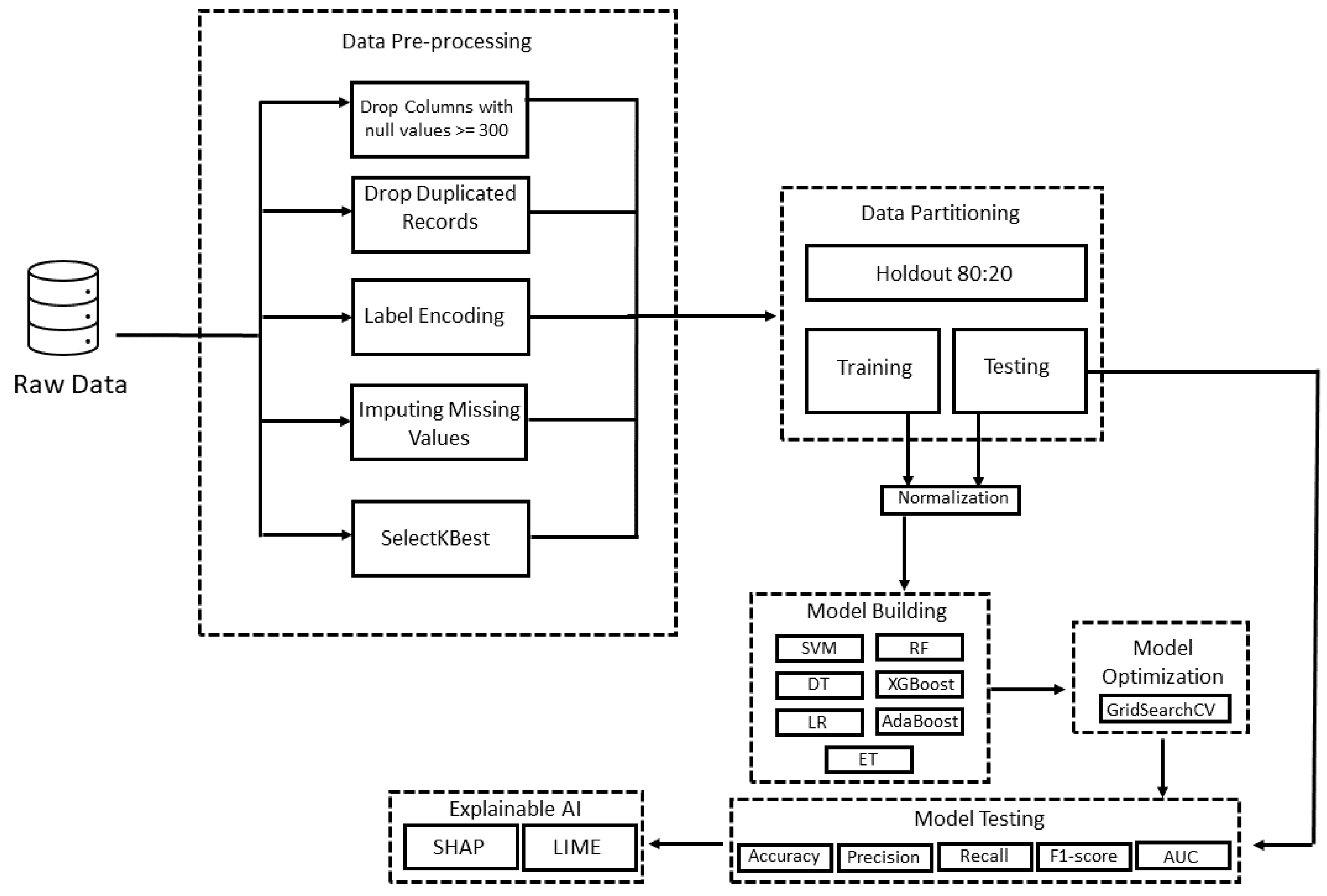
3. Materials and Methods
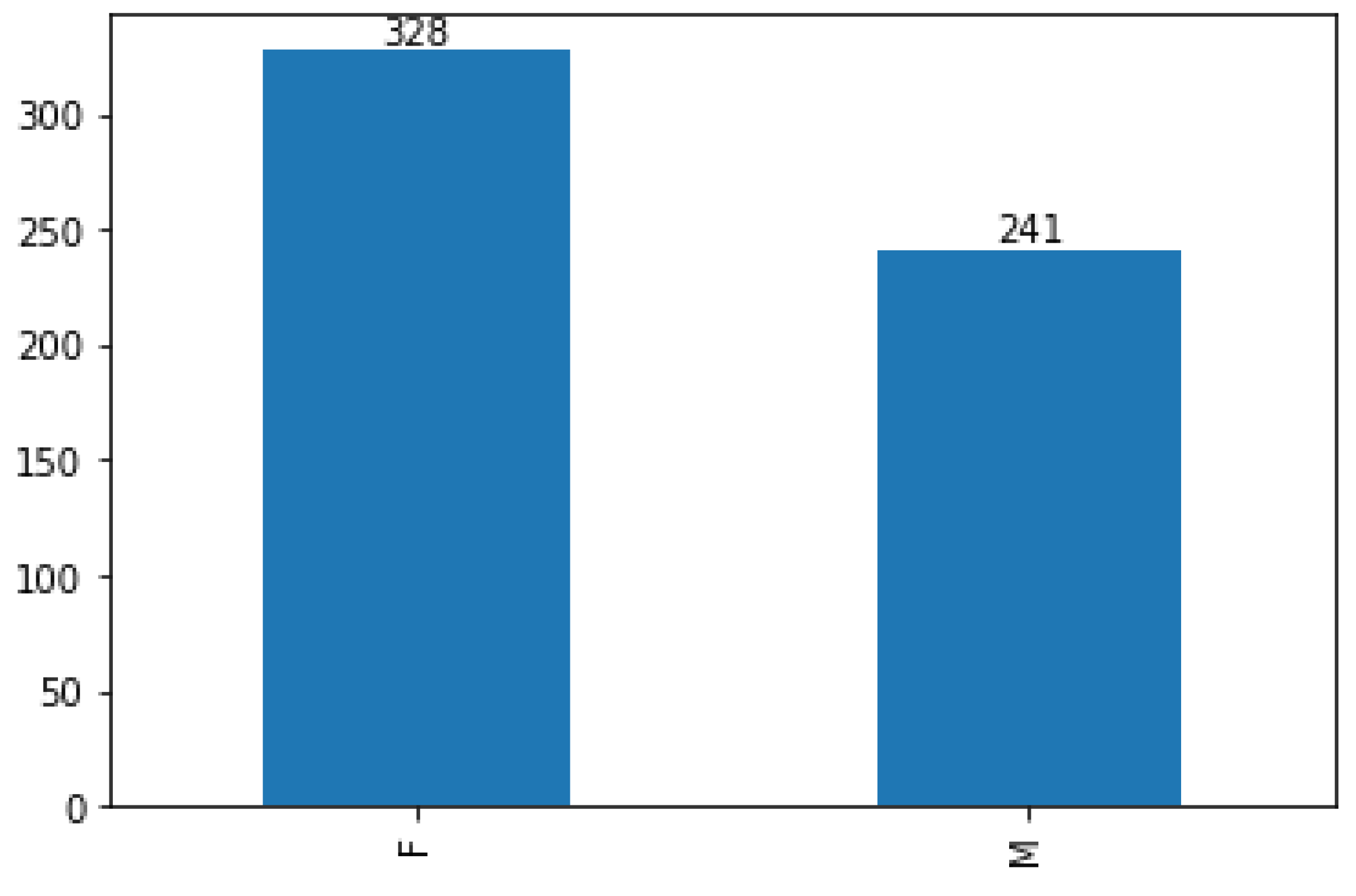
3.1. Data Description
3.2. Statistical Analysis
3.3. Data Pre-Processing
3.4. Description of Utilized Machine Learning Algorithms
3.4.1. Support Vector Machine (SVM)
3.4.2. Decision Tree (DT)
3.4.3. Logistic Regression (LR)
3.4.4. Random Forest (RF)
3.4.5. Extra Trees (ET)
3.4.6. Extreme Gradient Boosting (XGBoost)
3.4.7. Adaptive Boosting (AdaBoost)
3.5. Performance Measure
- TN indicates patients who were correctly identified as non-MS patients.
- TP indicates patients who were correctly identified as pwMS.
- FN indicates patients who were incorrectly identified as non-MS patients.
- FP indicates patients who were incorrectly identified as pwMS.
3.6. Optimization Strategy
4. Empirical Results
4.1. Interpretation of the Final Recommended Model
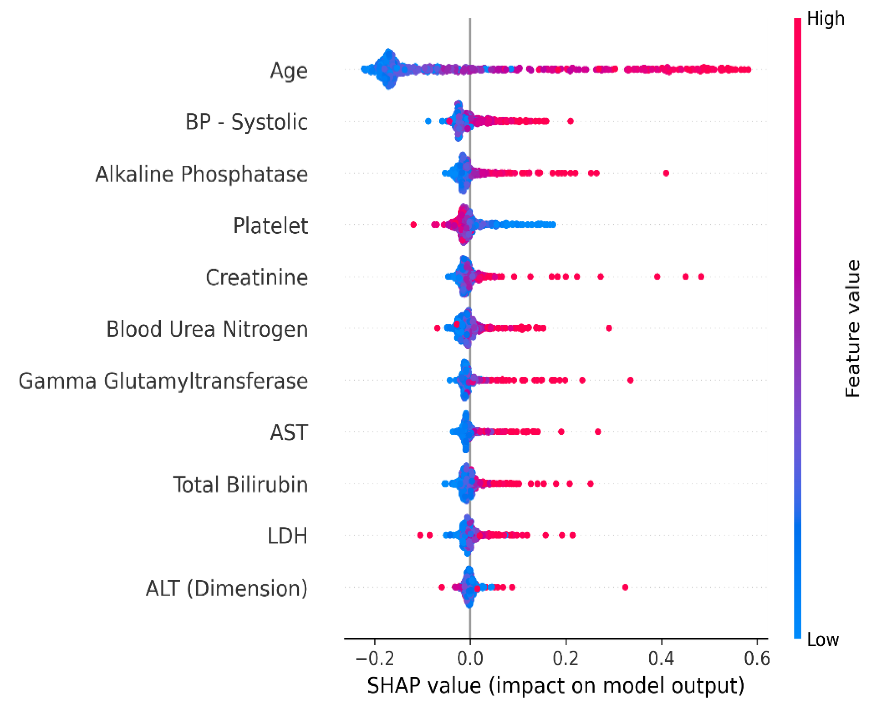
4.1.1. Shapley Additive Explanation (SHAP)
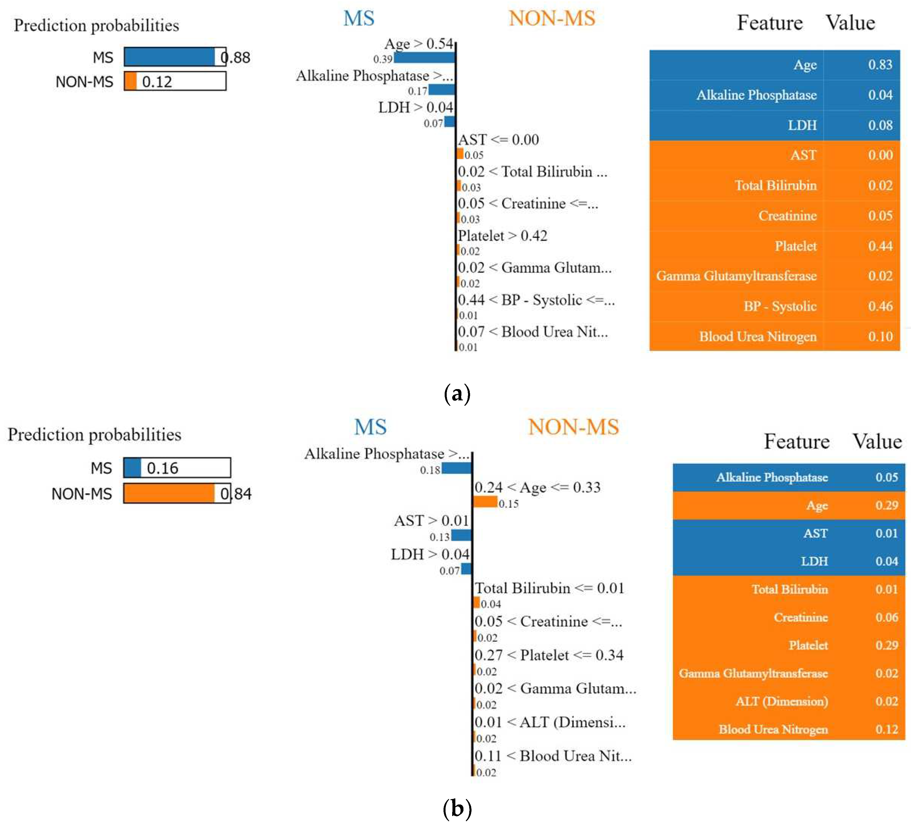
4.1.2. Local Interpretable Model-Agnostic Explanations (LIME)
5. Discussion
6. Conclusions
Supplementary Materials
Author Contributions
Funding
Institutional Review Board Statement
Informed Consent Statement
Data Availability Statement
Conflicts of Interest
References
- Noncommunicable Diseases. Available online: https://www.who.int/news-room/fact-sheets/detail/noncommunicable-diseases (accessed on 24 November 2022).
- Rappaport, S.M. Genetic Factors Are Not the Major Causes of Chronic Diseases. PLoS ONE 2016, 11, e0154387. [Google Scholar] [CrossRef]
- Morabia, A.; Abel, T. The WHO report “Preventing Chronic Diseases: A vital investment” and us. Soz. Praventivmed. 2006, 51, 74. [Google Scholar] [CrossRef]
- Walton, C.; King, R.; Rechtman, L.; Kaye, W.; Leray, E.; Marrie, R.A.; Robertson, N.; La Rocca, N.; Uitdehaag, B.; Van Der Mei, I.; et al. Rising prevalence of multiple sclerosis worldwide: Insights from the Atlas of MS, third edition. Mult. Scler. J. 2020, 26, 1816–1821. [Google Scholar] [CrossRef] [PubMed]
- Bunyan, R.; Al Otaibi, H.; Al Towaijri, G.; Karim, A.; Al Malik, Y.; Kalakatawi, M.; Alrajeh, S.; Al Mejally, M.; Algahtani, H. Rising prevalence of multiple sclerosis in Saudi Arabia, a descriptive study. BMC Neurol. 2020, 20, 49. [Google Scholar] [CrossRef]
- Multiple Sclerosis. Available online: https://www.moh.gov.sa/en/awarenessplateform/VariousTopics/Pages/MultipleSclerosis.aspx (accessed on 24 November 2022).
- Schaeffer, J.; Cossetti, C.; Mallucci, G.; Pluchino, S. Multiple Sclerosis. In Neurobiology of Brain Disorders: Biological Basis of Neurological and Psychiatric Disorders; Elsevier: Cambridge, MA, USA, 2015; pp. 497–520. [Google Scholar] [CrossRef]
- Murray, T.J. Diagnosis and treatment of multiple sclerosis. BMJ 2006, 332, 525–527. [Google Scholar] [CrossRef] [PubMed]
- Waubant, E. Improving Outcomes in Multiple Sclerosis Through Early Diagnosis and Effective Management. Prim. Care Companion CNS Disord. 2012, 14, 27363. [Google Scholar] [CrossRef]
- Aslam, N.; Khan, I.U.; Bashamakh, A.; Alghool, F.A.; Aboulnour, M.; Alsuwayan, N.M.; Alturaif, R.K.; Brahimi, S.; Aljameel, S.S.; Al Ghamdi, K. Multiple Sclerosis Diagnosis Using Machine Learning and Deep Learning: Challenges and Opportunities. Sensors 2022, 22, 7856. [Google Scholar] [CrossRef] [PubMed]
- Schmierer, K.; Parkes, H.G.; So, P.-W.; An, S.F.; Brandner, S.; Ordidge, R.; Yousry, T.A.; Miller, D.H. High field (9.4 Tesla) magnetic resonance imaging of cortical grey matter lesions in multiple sclerosis. Brain 2010, 133, 858–867. [Google Scholar] [CrossRef]
- Fangerau, T.; Schimrigk, S.; Haupts, M.; Kaeder, M.; Ahle, G.; Brune, N.; Klinkenberg, K.; Kotterba, S.; Mohring, M.; Sindern, E.; et al. Diagnosis of multiple sclerosis: Comparison of the Poser criteria and the new McDonald criteria. Acta Neurol. Scand. 2004, 109, 385–389. [Google Scholar] [CrossRef]
- Despotović, I.; Goossens, B.; Philips, W. MRI Segmentation of the Human Brain: Challenges, Methods, and Applications. Comput. Math. Methods Med. 2015, 2015, 1–23. [Google Scholar] [CrossRef]
- Arrieta, A.B.; Díaz-Rodríguez, N.; Del Ser, J.; Bennetot, A.; Tabik, S.; Barbado, A.; Garcia, S.; Gil-Lopez, S.; Molina, D.; Benjamins, R.; et al. Explainable Artificial Intelligence (XAI): Concepts, taxonomies, opportunities and challenges toward responsible AI. Inf. Fusion 2020, 58, 82–115. [Google Scholar] [CrossRef]
- Montolío, A.; Martín-Gallego, A.; Cegoñino, J.; Orduna, E.; Vilades, E.; Garcia-Martin, E.; del Palomar, A.P. Machine learning in diagnosis and disability prediction of multiple sclerosis using optical coherence tomography. Comput. Biol. Med. 2021, 133, 104416. [Google Scholar] [CrossRef] [PubMed]
- Montolío, A.; Cegoñino, J.; Garcia-Martin, E.; Pérez del Palomar, A. Comparison of Machine Learning Methods Using Spectralis OCT for Diagnosis and Disability Progression Prognosis in Multiple Sclerosis. Ann. Biomed. Eng. 2022, 50, 507–528. [Google Scholar] [CrossRef]
- Del Palomar, A.P.; Cegoñino, J.; Montolío, A.; Orduna, E.; Vilades, E.; Sebastián, B.; Pablo, L.E.; Garcia-Martin, E. Swept source optical coherence tomography to early detect multiple sclerosis disease. The use of machine learning techniques. PLoS ONE 2019, 14, e0216410. [Google Scholar] [CrossRef]
- Garcia-Martin, E.; Ortiz, M.; Boquete, L.; Sánchez-Morla, E.; Barea, R.; Cavaliere, C.; Vilades, E.; Orduna, E.; Rodrigo, M. Early diagnosis of multiple sclerosis by OCT analysis using Cohen’s d method and a neural network as classifier. Comput. Biol. Med. 2021, 129, 104165. [Google Scholar] [CrossRef] [PubMed]
- Ettema, R.; Lenders, M.W.P.M.; Vliegen, J.; Slettenaar, A.; Tjepkema-Cloostermans, M.C.; de Vos, C. Detecting multiple sclerosis via breath analysis using an eNose, a pilot study. J. Breath Res. 2021, 15, 027101. [Google Scholar] [CrossRef]
- Rocca, M.A.; Anzalone, N.; Storelli, L.; Del Poggio, A.; Cacciaguerra, L.; Manfredi, A.A.; Meani, A.; Filippi, M. Deep Learning on Conventional Magnetic Resonance Imaging Improves the Diagnosis of Multiple Sclerosis Mimics. Investig. Radiol. 2021, 56, 252–260. [Google Scholar] [CrossRef]
- Storelli, L.; Azzimonti, M.; Gueye, M.; Vizzino, C.M.; Preziosa, P.M.; Tedeschi, G.; De Stefano, N.M.; Pantano, P.M.; Filippi, M.; Rocca, M.A. A Deep Learning Approach to Predicting Disease Progression in Multiple Sclerosis Using Magnetic Resonance Imaging. Investig. Radiol. 2022, 57, 423–432. [Google Scholar] [CrossRef]
- Al Jannat, S.; Hoque, T.; Alam Supti, N.; Alam, A. Detection of Multiple Sclerosis using Deep Learning. In Proceedings of the 2021 Asian Conference on Innovation in Technology, ASIANCON 2021, Pune, India, 27–29 August 2021; pp. 1–8. [Google Scholar] [CrossRef]
- Alijamaat, A.; NikravanShalmani, A.; Bayat, P. Multiple sclerosis identification in brain MRI images using wavelet convolutional neural networks. Int. J. Imaging Syst. Technol. 2021, 31, 778–785. [Google Scholar] [CrossRef]
- sklearn.preprocessing. LabelEncoder—scikit-learn 1.1.3 documentation. Available online: https://scikit-learn.org/stable/modules/generated/sklearn.preprocessing.LabelEncoder.html (accessed on 24 November 2022).
- Bai, S.; Kolter, J.Z.; Koltun, V. An Empirical Evaluation of Generic Convolutional and Recurrent Networks for Sequence Modeling. arXiv 2018, arXiv:1803.01271. [Google Scholar]
- Zulfiker, S.; Kabir, N.; Biswas, A.A.; Nazneen, T.; Uddin, M.S. An in-depth analysis of machine learning approaches to predict depression. Curr. Res. Behav. Sci. 2021, 2, 100044. [Google Scholar] [CrossRef]
- Brereton, R.G.; Lloyd, G.R. Support Vector Machines for classification and regression. Analyst 2010, 135, 230–267. [Google Scholar] [CrossRef]
- Moguerza, J.M.; Muñoz, A. Support Vector Machines with Applications. Stat. Sci. 2006, 21, 322–336. [Google Scholar] [CrossRef]
- Battineni, G.; Chintalapudi, N.; Amenta, F. Machine learning in medicine: Performance calculation of dementia prediction by support vector machines (SVM). Inform. Med. Unlocked 2019, 16, 100200. [Google Scholar] [CrossRef]
- Rokach, L.; Maimon, O. Decision Trees. In Data Mining and Knowledge Discovery Handbook; Springer: Berlin/Heidelberg, Germany, 2005; pp. 165–192. [Google Scholar]
- Ashenden, S.K. The Era of Artificial Intelligence, Machine Learning, and Data Science in the Pharmaceutical Industry; Elsevier: London, UK, 2021. [Google Scholar] [CrossRef]
- Belyadi, H.; Haghighat, A. Machine Learning Guide for Oil and Gas Using Python: A Step-by-Step Breakdown with Data, Algorithms, Codes, and Applications; Gulf Professional Publishing: Oxford, UK, 2021. [Google Scholar] [CrossRef]
- Gislason, P.O.; Benediktsson, J.A.; Sveinsson, J.R. Random Forests for land cover classification. Pattern Recognit. Lett. 2006, 27, 294–300. [Google Scholar] [CrossRef]
- Krishnamoorthi, R.; Joshi, S.; Almarzouki, H.Z.; Shukla, P.K.; Rizwan, A.; Kalpana, C.; Tiwari, B. A Novel Diabetes Healthcare Disease Prediction Framework Using Machine Learning Techniques. J. Healthc. Eng. 2022, 2022, 1684017. [Google Scholar] [CrossRef]
- Geurts, P.; Ernst, D.; Wehenkel, L. Extremely randomized trees. Mach. Learn. 2006, 63, 3–42. [Google Scholar] [CrossRef]
- Paul, A.; Furmanchuk, A.; Liao, W.; Choudhary, A.; Agrawal, A. Property Prediction of Organic Donor Molecules for Photovoltaic Applications Using Extremely Randomized Trees. Mol. Inform. 2019, 38, e1900038. [Google Scholar] [CrossRef]
- Li, W.; Yin, Y.; Quan, X.; Zhang, H. Gene Expression Value Prediction Based on XGBoost Algorithm. Front. Genet. 2019, 10, 1077. [Google Scholar] [CrossRef]
- Sinha, N.K.; Khulal, M.; Gurung, M.; Lal, A. Developing A Web based System for Breast Cancer Prediction using XGboost Classifier. Int. J. Eng. Res. 2020, 9, 852–856. [Google Scholar] [CrossRef]
- Schapire, R.E. Explaining adaboost. In Empirical Inference; Springer: Berlin/Heidelberg, Germany, 2013; pp. 37–52. [Google Scholar] [CrossRef]
- Pandey, P.; Prabhakar, R. An analysis of machine learning techniques (J48 & AdaBoost)-for classification. In Proceedings of the 2016 1st India International Conference on Information Processing (IICIP), Delhi, India, 12–14 August 2016; pp. 1–6. [Google Scholar] [CrossRef]
- Gaitán, M.I.; Correale, J. Multiple Sclerosis Misdiagnosis: A Persistent Problem to Solve. Front. Neurol. 2019, 10, 466. [Google Scholar] [CrossRef] [PubMed]
- Solomon, A.J.; Naismith, R.T.; Cross, A.H. Misdiagnosis of multiple sclerosis: Impact of the 2017 McDonald criteria on clinical practice. Neurology 2018, 92, 26–33. [Google Scholar] [CrossRef] [PubMed]
- Kamath, U.; Liu, J. Explainable Artificial Intelligence: An Introduction to Interpretable Machine Learning; Springer: Berlin/Heidelberg, Germany, 2021. [Google Scholar] [CrossRef]
- Emmert-Streib, F.; Yli-Harja, O.; Dehmer, M. Explainable artificial intelligence and machine learning: A reality rooted perspective. WIREs Data Min. Knowl. Discov. 2020, 10, e1368. [Google Scholar] [CrossRef]
- Feng, D.-C.; Wang, W.-J.; Mangalathu, S.; Taciroglu, E. Interpretable XGBoost-SHAP Machine-Learning Model for Shear Strength Prediction of Squat RC Walls. J. Struct. Eng. 2021, 147, 04021173. [Google Scholar] [CrossRef]
- Alkadhim, H.A.; Amin, M.N.; Ahmad, W.; Khan, K.; Nazar, S.; Faraz, M.I.; Imran, M. Evaluating the Strength and Impact of Raw Ingredients of Cement Mortar Incorporating Waste Glass Powder Using Machine Learning and SHapley Additive ExPlanations (SHAP) Methods. Materials 2022, 15, 7344. [Google Scholar] [CrossRef] [PubMed]
- Gabbay, F.; Bar-Lev, S.; Montano, O.; Hadad, N. A LIME-Based Explainable Machine Learning Model for Predicting the Severity Level of COVID-19 Diagnosed Patients. Appl. Sci. 2021, 11, 10417. [Google Scholar] [CrossRef]
- Magesh, P.R.; Myloth, R.D.; Tom, R.J. An Explainable Machine Learning Model for Early Detection of Parkinson’s Disease using LIME on DaTSCAN Imagery. Comput. Biol. Med. 2020, 126, 104041. [Google Scholar] [CrossRef]
- Javaid, M.; Haleem, A.; Singh, R.P.; Suman, R.; Rab, S. Significance of machine learning in healthcare: Features, pillars and applications. Int. J. Intell. Networks 2022, 3, 58–73. [Google Scholar] [CrossRef]
- Kaur, P.; Sharma, M.; Mittal, M. Big Data and Machine Learning Based Secure Healthcare Framework. Procedia Comput. Sci. 2018, 132, 1049–1059. [Google Scholar] [CrossRef]
- Saudi Arabia Magnetic Resonance Imaging Market Size, Share, Trends, and Forecast 2027. Available online: https://www.techsciresearch.com/report/saudi-arabia-magnetic-resonance-imaging-market/8197.html (accessed on 22 February 2023).
- Johnson, P.M.; Recht, M.P.; Knoll, F. Improving the Speed of MRI with Artificial Intelligence. Semin. Musculoskelet. Radiol. 2020, 24, 012–020. [Google Scholar] [CrossRef]
- Hardy-Sosa, A.; León-Arcia, K.; Llibre-Guerra, J.J.; Berlanga-Acosta, J.; Baez, S.d.l.C.; Guillen-Nieto, G.; Valdes-Sosa, P.A. Diagnostic Accuracy of Blood-Based Biomarker Panels: A Systematic Review. Front. Aging Neurosci. 2022, 14, 103. [Google Scholar] [CrossRef] [PubMed]
- Goldman, M.D.; Min, S.; Lobo, J.M.; Sohn, M.-W. Retrospective cohort study of the relationship between systolic blood pressure variability and multiple sclerosis disability. BMJ Open 2020, 10, e034355. [Google Scholar] [CrossRef] [PubMed]
- Millar, J.H.; Merrett, J.D.; Dalby, A.M. Platelet stickiness in multiple sclerosis. J. Neurol. Neurosurg. Psychiatry 1966, 29, 187–189. [Google Scholar] [CrossRef]
- Tavazzi, B.; Batocchi, A.P.; Amorini, A.M.; Nociti, V.; D’Urso, S.; Longo, S.; Gullotta, S.; Picardi, M.; Lazzarino, G. Serum Metabolic Profile in Multiple Sclerosis Patients. Mult. Scler. Int. 2011, 2011, 167156. [Google Scholar] [CrossRef] [PubMed]


| Feature | Type |
|---|---|
| Sex | Categorical |
| Age | Integer |
| Anion Gap | Integer |
| ALT (Dimension) | Integer |
| LDH | Integer |
| White Blood Cells | Float |
| Red Blood Cells | Float |
| Hemoglobin | Float |
| Hematocrit | Float |
| Sodium | Integer |
| Potassium | Float |
| Chloride | Integer |
| Carbon Dioxide | Integer |
| Creatinine | Float |
| Total Protein | Float |
| Albumin | Float |
| Blood Urea Nitrogen | Integer |
| Total Bilirubin | Float |
| Direct Bilirubin | Float |
| Gamma Glutamyl transferase | Integer |
| MCV | Float |
| MCH | Float |
| MCHC | Float |
| Alkaline Phosphatase | Integer |
| RDW | Float |
| MPV | Float |
| AST | Integer |
| Lymphocyte—Instrument % | Float |
| Monocyte—Instrument % | Float |
| Lymphocyte—Instrument Abso | Float |
| Monocyte—Instrument Abso | Float |
| Neutrophil Granulocyte—Instrument % | Float |
| Neutrophil Granulocyte—Instrument Abso | Float |
| Platelet | Integer |
| Eosinophil—Instrument % | Float |
| Eosinophil—Instrument Abso | Float |
| Basophil—Instrument % | Float |
| Basophil—Instrument Abso | Float |
| BP—Systolic | Integer |
| Pulse Ox | Integer |
| Temperature | Float |
| Pulse | Integer |
| Respiratory Rate | Integer |
| BP—Diastolic | Integer |
| Class | Boolean |
| Feature | Mean | Standard Deviation | Min | 25th Quartile | 50th Quartile | 75th Quartile | Max | Missing Value Counts |
|---|---|---|---|---|---|---|---|---|
| Age | 43.28 | 16.71 | 13.00 | 30.00 | 38.00 | 55.00 | 89.00 | 0 |
| Anion Gap | 9.61 | 2.63 | 1.00 | 8.00 | 10.00 | 11.00 | 27.00 | 20 |
| ALT (Dimension) | 33.59 | 64.25 | 5.00 | 16.00 | 22.00 | 32.00 | 1278.00 | 12 |
| LDH | 182.51 | 131.29 | 95.00 | 142.75 | 164.00 | 187.00 | 2523.00 | 13 |
| White Blood Cells | 6.39 | 2.62 | 1.30 | 4.65 | 6.00 | 7.60 | 28.20 | 2 |
| Red Blood Cells | 4.68 | 0.69 | 1.91 | 4.26 | 4.69 | 5.13 | 6.72 | 2 |
| Hemoglobin | 12.80 | 2.14 | 5.80 | 11.50 | 12.90 | 14.40 | 18.50 | 2 |
| Hematocrit | 38.65 | 5.99 | 18.30 | 35.10 | 38.90 | 42.90 | 54.30 | 2 |
| Sodium | 140.00 | 2.69 | 125.00 | 138.00 | 140.00 | 141.00 | 157.00 | 20 |
| Potassium | 4.30 | 0.43 | 3.10 | 4.00 | 4.30 | 4.50 | 6.10 | 20 |
| Chloride | 103.86 | 2.51 | 92.00 | 102.00 | 104.00 | 105.00 | 121.00 | 20 |
| Carbon Dioxide | 26.43 | 3.14 | 13.00 | 25.00 | 27.00 | 28.00 | 44.00 | 20 |
| Creatinine | 0.89 | 0.97 | 0.15 | 0.62 | 0.72 | 0.89 | 12.23 | 19 |
| Total Protein | 7.31 | 0.64 | 3.10 | 7.00 | 7.30 | 7.70 | 8.90 | 13 |
| Albumin | 3.80 | 0.52 | 1.70 | 3.60 | 3.90 | 4.10 | 5.10 | 13 |
| Blood Urea Nitrogen | 13.81 | 9.37 | 3.00 | 9.00 | 12.00 | 15.00 | 83.00 | 20 |
| Total Bilirubin | 0.62 | 0.98 | 0.10 | 0.30 | 0.40 | 0.70 | 16.70 | 13 |
| Direct Bilirubin | 0.21 | 0.56 | 0.05 | 0.09 | 0.12 | 0.20 | 11.10 | 13 |
| Gamma Glutamyl Transferase | 49.85 | 104.49 | 4.00 | 19.00 | 27.00 | 43.00 | 1296.00 | 13 |
| MCV | 83.41 | 8.81 | 48.9 | 79.35 | 84.50 | 89.20 | 133.00 | 2 |
| MCH | 27.48 | 3.29 | 15.30 | 25.80 | 28.00 | 29.80 | 40.90 | 2 |
| MCHC | 33.00 | 1.39 | 27.70 | 32.10 | 33.10 | 34.00 | 36.20 | 2 |
| Alkaline Phosphatase | 85.00 | 100.13 | 21.00 | 58.00 | 70.00 | 90.00 | 1881.00 | 13 |
| RDW | 14.39 | 2.25 | 10.40 | 13.10 | 13.80 | 15.00 | 30.90 | 2 |
| MPV | 8.77 | 1.02 | 6.00 | 8.10 | 8.70 | 9.40 | 12.70 | 4 |
| AST | 34.97 | 157.53 | 5.00 | 15.00 | 18.00 | 24.00 | 2560.00 | 12 |
| Lymphocyte—Instrument % | 33.91 | 11.95 | 2.00 | 26.60 | 34.30 | 42.30 | 69.20 | 43 |
| Monocyte—Instrument % | 8.78 | 2.54 | 1.20 | 7.00 | 8.40 | 10.17 | 19.20 | 43 |
| Lymphocyte—Instrument Abso | 2.06 | 0.82 | 0.20 | 1.50 | 2.00 | 2.60 | 5.40 | 43 |
| Monocyte—Instrument Abso | 0.54 | 0.20 | 0.10 | 0.40 | 0.50 | 0.60 | 1.60 | 43 |
| Neutrophil Granulocyte—Instrument % | 53.87 | 13.37 | 17.70 | 45.30 | 53.30 | 60.70 | 91.90 | 43 |
| Neutrophil Granulocyte—Instrument Abso | 3.69 | 2.00 | 0.70 | 2.40 | 3.30 | 4.60 | 12.30 | 43 |
| Platelet | 254.80 | 81.72 | 27.00 | 204.00 | 249.00 | 302.25 | 679.00 | 9 |
| Eosinophil—Instrument % | 2.67 | 2.00 | 0.00 | 1.30 | 2.20 | 3.60 | 13.70 | 43 |
| Eosinophil—Instrument Abso | 0.16 | 0.15 | 0.00 | 0.10 | 0.10 | 0.20 | 1.00 | 43 |
| Basophil—Instrument % | 0.60 | 0.42 | 0.00 | 0.30 | 0.50 | 0.80 | 2.80 | 43 |
| Basophil—Instrument Abso | 0.03 | 0.04 | 0.00 | 0.00 | 0.00 | 0.10 | 0.20 | 43 |
| BP—Systolic | 126.30 | 18.01 | 58.00 | 115.00 | 124.00 | 137.00 | 191.00 | 110 |
| Pulse Ox | 98.70 | 2.56 | 53.00 | 98.00 | 99.00 | 100.00 | 100.00 | 123 |
| Temperature | 36.76 | 0.29 | 35.40 | 36.60 | 36.80 | 36.90 | 39.30 | 120 |
| Pulse | 83.40 | 13.00 | 50.00 | 75.00 | 83.00 | 89.00 | 132.00 | 111 |
| Respiratory Rate | 19.59 | 1.29 | 15.00 | 18.00 | 20.00 | 20.00 | 28.00 | 110 |
| BP—Diastolic | 76.00 | 10.92 | 32.00 | 69.00 | 76.00 | 84.00 | 107.00 | 110 |
| Classifier | Hyperparameter | Optimal Hyperparameter |
|---|---|---|
| SVM | C | 1 |
| gamma | 1 | |
| kernel | rbf | |
| DT | criterion | gini |
| max_depth | 2 | |
| min_samples_leaf | 3 | |
| max_leaf_nodes | 19 | |
| LR | penalty | l2 |
| class_weight | dict | |
| C | 1 | |
| RF | max_depth | 6 |
| n_estimators | 150 | |
| criterion | entropy | |
| max_leaf_nodes | None | |
| min_samples_leaf | 3 | |
| XGBoost | n_estimators | 80 |
| learning_rate | 0.1 | |
| booster | gbtree | |
| gamma | 0.3 | |
| AdaBoost | n_estimators | 100 |
| learning_rate | 0.2 | |
| algorithm | SAMME.R | |
| ET | n_estimators | 450 |
| max_depth | 12 | |
| max_leaf_nodes | None | |
| min_samples_leaf | 1 |
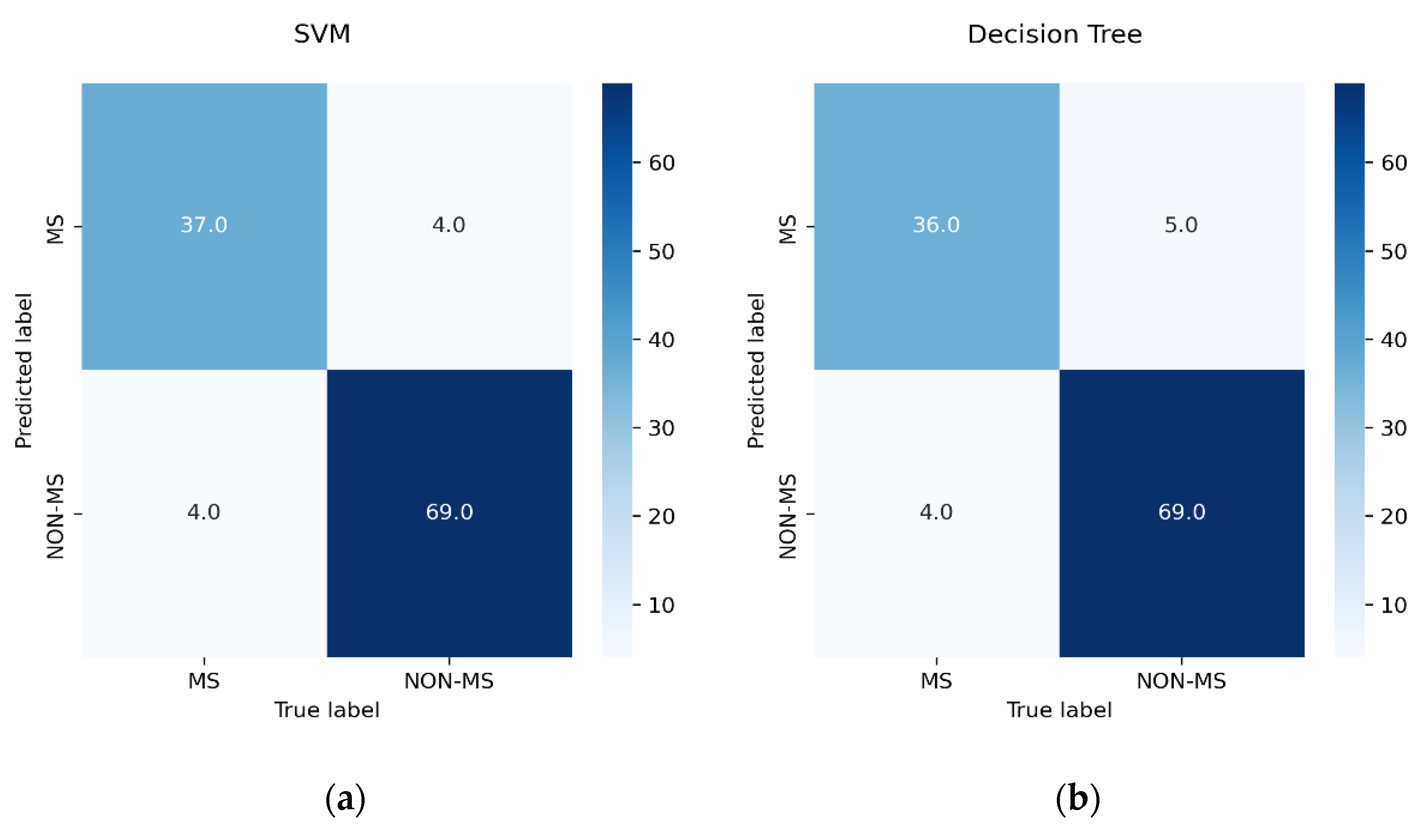
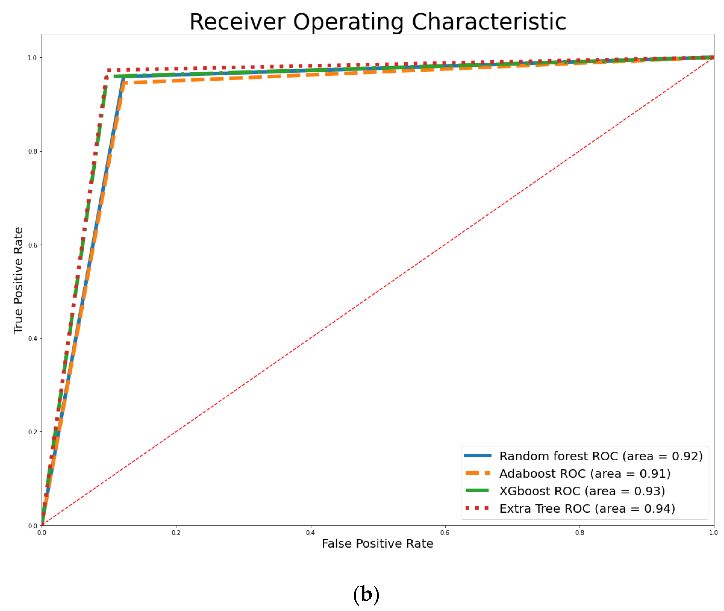
| Classifier | Training Accuracy | Testing Accuracy | Precision | Recall | F1-Score |
|---|---|---|---|---|---|
| SVM | 89.01% | 92.98% | 94.52% | 94.52% | 94.52% |
| DT | 88.13% | 92.11% | 93.24% | 94.52% | 93.88% |
| LR | 87.69% | 92.98% | 94.52% | 94.52% | 94.52% |
| RF | 92.53% | 92.98% | 93.33% | 95.89% | 94.59% |
| XGBoost | 99.56% | 93.86% | 94.59% | 95.89% | 95.24% |
| AdaBoost | 93.24% | 92.11% | 93.24% | 94.52% | 93.88% |
| ET | 95.82% | 94.74% | 94.67% | 97.26% | 95.95% |
Disclaimer/Publisher’s Note: The statements, opinions and data contained in all publications are solely those of the individual author(s) and contributor(s) and not of MDPI and/or the editor(s). MDPI and/or the editor(s) disclaim responsibility for any injury to people or property resulting from any ideas, methods, instructions or products referred to in the content. |
© 2023 by the authors. Licensee MDPI, Basel, Switzerland. This article is an open access article distributed under the terms and conditions of the Creative Commons Attribution (CC BY) license (https://creativecommons.org/licenses/by/4.0/).
Share and Cite
Olatunji, S.O.; Alsheikh, N.; Alnajrani, L.; Alanazy, A.; Almusairii, M.; Alshammasi, S.; Alansari, A.; Zaghdoud, R.; Alahmadi, A.; Basheer Ahmed, M.I.; et al. Comprehensible Machine-Learning-Based Models for the Pre-Emptive Diagnosis of Multiple Sclerosis Using Clinical Data: A Retrospective Study in the Eastern Province of Saudi Arabia. Int. J. Environ. Res. Public Health 2023, 20, 4261. https://doi.org/10.3390/ijerph20054261
Olatunji SO, Alsheikh N, Alnajrani L, Alanazy A, Almusairii M, Alshammasi S, Alansari A, Zaghdoud R, Alahmadi A, Basheer Ahmed MI, et al. Comprehensible Machine-Learning-Based Models for the Pre-Emptive Diagnosis of Multiple Sclerosis Using Clinical Data: A Retrospective Study in the Eastern Province of Saudi Arabia. International Journal of Environmental Research and Public Health. 2023; 20(5):4261. https://doi.org/10.3390/ijerph20054261
Chicago/Turabian StyleOlatunji, Sunday O., Nawal Alsheikh, Lujain Alnajrani, Alhatoon Alanazy, Meshael Almusairii, Salam Alshammasi, Aisha Alansari, Rim Zaghdoud, Alaa Alahmadi, Mohammed Imran Basheer Ahmed, and et al. 2023. "Comprehensible Machine-Learning-Based Models for the Pre-Emptive Diagnosis of Multiple Sclerosis Using Clinical Data: A Retrospective Study in the Eastern Province of Saudi Arabia" International Journal of Environmental Research and Public Health 20, no. 5: 4261. https://doi.org/10.3390/ijerph20054261
APA StyleOlatunji, S. O., Alsheikh, N., Alnajrani, L., Alanazy, A., Almusairii, M., Alshammasi, S., Alansari, A., Zaghdoud, R., Alahmadi, A., Basheer Ahmed, M. I., Ahmed, M. S., & Alhiyafi, J. (2023). Comprehensible Machine-Learning-Based Models for the Pre-Emptive Diagnosis of Multiple Sclerosis Using Clinical Data: A Retrospective Study in the Eastern Province of Saudi Arabia. International Journal of Environmental Research and Public Health, 20(5), 4261. https://doi.org/10.3390/ijerph20054261