
Is Active Moss Biomonitoring Comparable to Air Filter Standard Sampling?

 ,
, 
 , and
, and 
Abstract
:
1. Introduction
2. Materials and Methods
3. Results
4. Discussion
5. Conclusions
Supplementary Materials
Author Contributions
Funding
Institutional Review Board Statement
Informed Consent Statement
Data Availability Statement
Acknowledgments
Conflicts of Interest
References
- Li, H.H.; Chen, L.J.; Yu, L.; Guo, Z.B.; Shan, C.Q.; Lin, J.Q.; Gu, Y.G.; Yang, Z.B.; Yang, Y.X.; Shao, J.R.; et al. Pollution characteristics and risk assessment of human exposure to oral bioaccessibility of heavy metals via urban street dusts from different functional areas in Chengdu, China. Sci. Total Environ. 2017, 586, 1076–1084. [Google Scholar] [CrossRef] [PubMed]
- Chen, S.; Jiang, N.; Huang, J.; Zang, Z.; Guan, X.; Ma, X.; Luo, Y.; Li, J.; Zhang, X.; Zhang, Y. Estimations of indirect and direct anthropogenic dust emission at the global scale. Atmos. Environ. 2019, 200, 50–60. [Google Scholar] [CrossRef]
- Arditsoglou, A.; Samara, C. Levels of total suspended particulate matter and major trace elements in Kosovo: A source identification and apportionment study. Chemosphere 2005, 59, 669–678. [Google Scholar] [CrossRef] [PubMed]
- Després, V.R.; Nowoisky, J.F.; Klose, M.; Conrad, R.; Andreae, M.O.; Pöschl, U. Characterization of primary biogenic aerosol particles in urban, rural, and high-alpine air by DNA sequence and restriction fragment analysis of ribosomal RNA genes. Biogeosciences 2007, 4, 1127–1141. [Google Scholar] [CrossRef] [Green Version]
- Bakolis, I.; Hammoud, R.; Stewart, R.; Beevers, S.; Dajnak, D.; MacCrimmon, S.; Broadbent, M.; Pritchard, M.; Shiode, N.; Fecht, D.; et al. Mental health consequences of urban air pollution: Prospective population-based longitudinal survey. Soc. Psychiatry Psychiatr. Epidemiol. 2021, 56, 1587–1599. [Google Scholar] [CrossRef]
- Ma, J.; Ding, Y.; Cheng, J.C.P.; Jiang, F.; Tan, Y.; Gan, V.J.L.; Wan, Z. Identification of high impact factors of air quality on a national scale using big data and machine learning techniques. J. Clean. Prod. 2020, 244, 118955. [Google Scholar] [CrossRef]
- Kim, J.; Jeong, U.; Ahn, M.H.; Kim, J.H.; Park, R.J.; Lee, H.; Song, C.H.; Choi, Y.S.; Lee, K.H.; Yoo, J.M.; et al. New era of air quality monitoring from space: Geostationary environment monitoring spectrometer (GEMS). Bull. Am. Meteorol. Soc. 2020, 101, E1–E22. [Google Scholar] [CrossRef] [Green Version]
- Sheikh, A. Improving air quality needs to be a policy priority for governments globally. PLoS Med. 2020, 17, 10–12. [Google Scholar] [CrossRef] [Green Version]
- Vodonos, A.; Kloog, I.; Boehm, L.; Novack, V. The impact of exposure to particulate air pollution from non-Anthropogenic sources on hospital admissions due to pneumonia. Eur. Respir. J. 2016, 48, 1791–1794. [Google Scholar] [CrossRef] [Green Version]
- Kermani, M.; Jonidi Jafari, A.; Gholami, M.; Arfaeinia, H.; Shahsavani, A.; Fanaei, F. Characterization, possible sources and health risk assessment of PM2.5-bound Heavy Metals in the most industrial city of Iran. J. Environ. Heal. Sci. Eng. 2021, 19, 151–163. [Google Scholar] [CrossRef]
- Silva da Silva, C.; Rossato, J.M.; Vaz Rocha, J.A.; Vargas, V.M.F. Characterization of an area of reference for inhalable particulate matter (PM2.5) associated with genetic biomonitoring in children. Mutat. Res. Genet. Toxicol. Environ. Mutagen. 2015, 778, 44–55. [Google Scholar] [CrossRef] [PubMed]
- Liu, C.; Zhang, Y. Relations between indoor and outdoor PM2.5 and constituent concentrations. Front. Environ. Sci. Eng. 2019, 13, 1–20. [Google Scholar] [CrossRef]
- Wilson, W.E.; Chow, J.C.; Claiborn, C.; Fusheng, W.; Engelbrecht, J.; Watson, J.G. Monitoring of particulate matter outdoors. Chemosphere 2002, 49, 1009–1043. [Google Scholar] [CrossRef]
- Ali, M.; Athar, M. Air pollution due to traffic, air quality monitoring along three sections of National Highway N-5, Pakistan. Environ. Monit. Assess. 2008, 136, 219–226. [Google Scholar] [CrossRef] [PubMed]
- Schroeder, W.H.; Dobson, M.; Kane, D.M.; Johnson, N.D. Toxic Trace Elements Associated With Airborne Pariacnlaie Matter: A Review. J. Air Pollut. Control Assoc. 1987, 37, 1267–1285. [Google Scholar]
- Petrovský, E.; Zbořil, R.; Grygar, T.M.; Kotlík, B.; Novák, J.; Kapička, A.; Grison, H. Magnetic particles in atmospheric particulate matter collected at sites with different level of air pollution. Stud. Geophys. Geod. 2013, 57, 755–770. [Google Scholar] [CrossRef]
- Matos, P.; Vieira, J.; Rocha, B.; Branquinho, C.; Pinho, P. Modeling the provision of air-quality regulation ecosystem service provided by urban green spaces using lichens as ecological indicators. Sci. Total Environ. 2019, 665, 521–530. [Google Scholar] [CrossRef]
- Almeida, S.M.; Ramos, C.A.; Marques, A.M.; Silva, A.V.; Freitas, M.C.; Farinha, M.M.; Reis, M.; Marques, A.P. Use of INAA and PIXE for multipollutant air quality assessment and management. J. Radioanal. Nucl. Chem. 2012, 294, 343–347. [Google Scholar] [CrossRef]
- Stankovic, S.; Kalaba, P.; Stankovic, A.R. Biota as toxic metal indicators. Environ. Chem. Lett. 2014, 12, 63–84. [Google Scholar] [CrossRef]
- Hewitt, C.N.; Ashworth, K.; MacKenzie, A.R. Using green infrastructure to improve urban air quality (GI4AQ). Ambio 2020, 49, 62–73. [Google Scholar] [CrossRef] [Green Version]
- Floreani, F.; Barago, N.; Acquavita, A.; Covelli, S.; Skert, N.; Higueras, P. Spatial distribution and biomonitoring of atmospheric mercury concentrations over a contaminated coastal lagoon (Northern Adriatic, Italy). Atmosphere 2020, 11, 1280. [Google Scholar] [CrossRef]
- Kempter, H.; Krachler, M.; Shotyk, W.; Zaccone, C. Validating modelled data on major and trace element deposition in southern Germany using Sphagnum moss. Atmos. Environ. 2017, 167, 656–664. [Google Scholar] [CrossRef]
- Zarazúa-Ortega, G.; Poblano-Bata, J.; Tejeda-Vega, S.; Ávila-Pérez, P.; Zepeda-Gómez, C.; Ortiz-Oliveros, H.; Macedo-Miranda, G. Assessment of spatial variability of heavy metals in metropolitan zone of toluca valley, Mexico, using the biomonitoring technique in mosses and TXRF analysis. Sci. World J. 2013, 2013, 1–7. [Google Scholar] [CrossRef] [PubMed]
- Rai, P.K. Impacts of particulate matter pollution on plants: Implications for environmental biomonitoring. Ecotoxicol. Environ. Saf. 2016, 129, 120–136. [Google Scholar] [CrossRef] [PubMed]
- Clough, W.S. The deposition of particles on moss and grass surfaces. Atmos. Environ. 1975, 9, 1113–1119. [Google Scholar] [CrossRef]
- Ştefănuţ, S.; Manole, A.; Ion, M.C.; Constantin, M.; Banciu, C.; Onete, M.; Manu, M.; Vicol, I.; Moldoveanu, M.M.; Maican, S.; et al. Developing a novel warning-informative system as a tool for environmental decision-making based on biomonitoring. Ecol. Indic. 2018, 89, 480–487. [Google Scholar] [CrossRef]
- Ștefănuț, S.; Öllerer, K.; Manole, A.; Ion, M.C.; Constantin, M.; Banciu, C.; Maria, G.M.; Florescu, L.I. National environmental quality assessment and monitoring of atmospheric heavy metal pollution—A moss bag approach. J. Environ. Manag. 2019, 248, 109224. [Google Scholar] [CrossRef]
- Iodice, P.; Adamo, P.; Capozzi, F.; Di Palma, A.; Senatorea, A.; Spagnuolo, V.; Giordano, S. Air pollution monitoring using emission inventories combined with the moss bag approach. Sci. Total Environ. 2016, 541, 1410–1419. [Google Scholar] [CrossRef]
- Vanicela, B.D.; Nebel, M.; Stephan, M.; Riethmüller, C.; Gresser, G.T. Quantitative analysis of fine dust particles on moss surfaces under laboratory conditions using the example of Brachythecium rutabulum. Environ. Sci. Pollut. Res. 2021, 28, 51763–51771. [Google Scholar] [CrossRef]
- Vuković, G.; Aničić Uroševic, M.; Razumenić, I.; Kuzmanoski, M.; Pergal, M.; Škrivanj, S.; Popović, A. Air quality in urban parking garages (PM10, major and trace elements, PAHs): Instrumental measurements vs. active moss biomonitoring. Atmos. Environ. 2014, 85, 31–40. [Google Scholar] [CrossRef]
- Capozzi, F.; Sorrentino, M.C.; Di Palma, A.; Mele, F.; Arena, C.; Adamo, P.; Spagnuolo, V.; Giordano, S. Implication of vitality, seasonality and specific leaf area on PAH uptake in moss and lichen transplanted in bags. Ecol. Indic. 2020, 108, 105727. [Google Scholar] [CrossRef]
- Markert, B. From biomonitoring to integrated observation of the environment—The multi-markered bioindication concept. Ecol. Chem. Eng. S 2008, 15, 315–333. [Google Scholar]
- Sheppard, P.R.; Speakman, R.J.; Farris, C.; Witten, M.L. Multiple environmental monitoring techniques for assessing spatial patterns of airborne tungsten. Environ. Sci. Technol. 2007, 41, 406–410. [Google Scholar] [CrossRef] [PubMed]
- Pöykiö, R. Assessing Industrial Pollution by Means of Environmental Samples in the Kemi-Tornio Region; Oulu University Press: Oulu, Finland, 2002; ISBN 9514268709. [Google Scholar]
- Kupiainen, K.; Tervahattu, H. The effect of traction sanding on urban suspended particles in Finland. Environ. Monit. Assess. 2004, 93, 287–300. [Google Scholar] [CrossRef] [PubMed]
- Harmens, H.; Frontasyeva, M. Heavy Metals, Nitrogen and POPs in European Mosses: 2020 Survey; ICP Vegetation: Lancester, UK, 2020. [Google Scholar]
- Świsłowski, P.; Kosior, G.; Rajfur, M. The influence of preparation methodology on the concentrations of heavy metals in Pleurozium schreberi moss samples prior to use in active biomonitoring studies. Environ. Sci. Pollut. Res. 2021, 28, 10068–10076. [Google Scholar] [CrossRef]
- European Commission. EN 12341:2014 Ambient Air—Standard Gravimetric Measurement Method for the Determination of the PM10 or PM2,5 Mass Concentration of Suspended Particulate Matter; Austrian Standards International: Vienna, Austria, 2014. [Google Scholar]
- Gerboles, M.; Buzica, D.; Brown, R.J.C.; Yardley, R.E.; Hanus-Illnar, A.; Salfinger, M.; Vallant, B.; Adriaenssens, E.; Claeys, N.; Roekens, E.; et al. Interlaboratory comparison exercise for the determination of As, Cd, Ni and Pb in PM10 in Europe. Atmos. Environ. 2011, 45, 3488–3499. [Google Scholar] [CrossRef]
- Thermo Fisher Scientific Inc. iCE 3000 Series AA Spectrometers Operator’s Manual; Thermo Scientific: New York, NY, USA, 2011; Volume 44, pp. 1, 7–18. [Google Scholar]
- Rajfur, M.; Świsłowski, P.; Nowainski, F.; Śmiechowicz, B. Mosses as Biomonitor of Air Pollution with Analytes Originating from Tobacco Smoke. Chem. Didact. Ecol. Metrol. 2018, 23, 127–136. [Google Scholar] [CrossRef] [Green Version]
- Šraj Kržič, N.; Gaberščik, A. Photochemical efficiency of amphibious plants in an intermittent lake. Aquat. Bot. 2005, 83, 281–288. [Google Scholar] [CrossRef]
- Aitchison, J. The Statistical Analysis of Compositional Data; The Blackburn Press: Caldwell, NJ, USA, 2003. [Google Scholar]
- Pawlowsky-Glahn, V.; Buccianti, A. Compositional Data Analysis. Theory and Applications; John Wiley & Sons: London, UK, 2011. [Google Scholar]
- R Core Team. R: A Language and Environment for Statistical Computing; R Foundation for Statistical Computing: Vienna, Austria, 2021. [Google Scholar]
- Palarea-Albaladejo, J.; Martín-Fernández, J.A. ZCompositions—R package for multivariate imputation of left-censored data under a compositional approach. Chemom. Intell. Lab. Syst. 2015, 143, 85–96. [Google Scholar] [CrossRef]
- Chambers, J.M.; Hastie, T. Statistical Models in S; Wadsworth\& Brooks/Cole computer science series; Chapman & Hall: New York, NY, USA, 1993; ISBN 9780534167646. [Google Scholar]
- Kosior, G.; Frontasyeva, M.; Ziembik, Z.; Zincovscaia, I.; Dołhańczuk-Śródka, A.; Godzik, B. The Moss Biomonitoring Method and Neutron Activation Analysis in Assessing Pollution by Trace Elements in Selected Polish National Parks. Arch. Environ. Contam. Toxicol. 2020, 79, 310–320. [Google Scholar] [CrossRef]
- Kłos, A.; Ziembik, Z.; Rajfur, M.; Dołhańczuk-Śródka, A.; Bochenek, Z.; Bjerke, J.W.; Tømmervik, H.; Zagajewski, B.; Ziółkowski, D.; Jerz, D.; et al. Using moss and lichens in biomonitoring of heavy-metal contamination of forest areas in southern and north-eastern Poland. Sci. Total Environ. 2018, 627, 438–449. [Google Scholar] [CrossRef] [PubMed]
- Olszowski, T.; Bozym, M. Pilot study on using an alternative method of estimating emission of heavy metals from wood combustion. Atmos. Environ. 2014, 94, 22–27. [Google Scholar] [CrossRef]
- Rogova, N.; Ryzhakova, N.; Gusvitskii, K.; Eruntsov, V. Studying the influence of seasonal conditions and period of exposure on trace element concentrations in the moss-transplant Pylaisia polyantha. Environ. Monit. Assess. 2021, 193, 1–9. [Google Scholar] [CrossRef] [PubMed]
- Węgrzyn, M.H.; Fałowska, P.; Alzayany, K.; Waszkiewicz, K.; Dziurowicz, P.; Wietrzyk-Pełka, P. Seasonal Changes in the Photosynthetic Activity of Terrestrial Lichens and Mosses in the Lichen Scots Pine Forest Habitat. Diversity 2021, 13, 642. [Google Scholar] [CrossRef]
- Sujetovienė, G.; Galinytė, V. Effects of the urban environmental conditions on the physiology of lichen and moss. Atmos. Pollut. Res. 2016, 7, 611–618. [Google Scholar] [CrossRef]
- Romańska, M. Impact of water stress on physiological processes of moss Polytrichum piliferum Hedw. Ann. Univ. Paedagog. Cracoviensis Stud. Naturae 2020, 129–141. [Google Scholar] [CrossRef]
- Bargagli, R. Moss and lichen biomonitoring of atmospheric mercury: A review. Sci. Total Environ. 2016, 572, 216–231. [Google Scholar] [CrossRef]
- Diener, A.; Mudu, P. How can vegetation protect us from air pollution? A critical review on green spaces’ mitigation abilities for air-borne particles from a public health perspective—With implications for urban planning. Sci. Total Environ. 2021, 796, 148605. [Google Scholar] [CrossRef]
- González, A.G.; Pokrovsky, O.S. Metal adsorption on mosses: Toward a universal adsorption model. J. Colloid Interface Sci. 2014, 415, 169–178. [Google Scholar] [CrossRef] [Green Version]
- Sabovljević, M.S.; Weidinger, M.; Sabovljević, A.D.; Stanković, J.; Adlassnig, W.; Lang, I. Metal accumulation in the acrocarp moss Atrichum undulatum under controlled conditions. Environ. Pollut. 2020, 256, 1–8. [Google Scholar] [CrossRef]
- Culicov, O.A.; Mocanu, R.; Frontasyeva, M.V.; Yurukova, L.; Steinnes, E. Active moss biomonitoring applied to an industrial site in Romania: Relative accumulation of 36 elements in moss-bags. Environ. Monit. Assess. 2005, 108, 229–240. [Google Scholar] [CrossRef] [PubMed]
- Onianwa, P.C. Monitoring atmospheric metal pollution: A review of the use of mosses as indicators. Environ. Monit. Assess. 2001, 71, 13–50. [Google Scholar] [CrossRef] [PubMed]
- Aydoğan, S.; Erdağ, B.; Yildiz Aktaş, L. Bioaccumulation and oxidative stress impact of Pb, Ni, Cu, and Cr heavy metals in two bryophyte species, Pleurochaete squarrosa and timmiella barbuloides. Turk. J. Botany 2017, 41, 464–475. [Google Scholar] [CrossRef]
- Hussain, S.; Hoque, R.R. Biomonitoring of metallic air pollutants in unique habitations of the Brahmaputra Valley using moss species—Atrichum angustatum: Spatiotemporal deposition patterns and sources. Environ. Sci. Pollut. Res. 2022, 29, 10617–10634. [Google Scholar] [CrossRef] [PubMed]
- Kempter, H.; Krachler, M.; Shotyk, W.; Zaccone, C. Major and trace elements in Sphagnum moss from four southern German bogs, and comparison with available moss monitoring data. Ecol. Indic. 2017, 78, 19–25. [Google Scholar] [CrossRef]
- Aničić, M.; Tomašević, M.; Tasić, M.; Rajšić, S.; Popović, A.; Frontasyeva, M.V.; Lierhagen, S.; Steinnes, E. Monitoring of trace element atmospheric deposition using dry and wet moss bags: Accumulation capacity versus exposure time. J. Hazard. Mater. 2009, 171, 182–188. [Google Scholar] [CrossRef] [PubMed]
- Vuković, G.; Urošević, M.A.; Pergal, M.; Janković, M.; Goryainova, Z.; Tomašević, M.; Popović, A. Residential heating contribution to level of air pollutants (PAHs, major, trace, and rare earth elements): A moss bag case study. Environ. Sci. Pollut. Res. 2015, 22, 18956–18966. [Google Scholar] [CrossRef]
- Hu, R.; Yan, Y.; Zhou, X.; Wang, Y.; Fang, Y. Monitoring heavy metal contents with Sphagnum junghuhnianum moss bags in relation to traffic volume in Wuxi, China. Int. J. Environ. Res. Public Health 2018, 15, 374. [Google Scholar] [CrossRef] [Green Version]
- Capozzi, F.; Adamo, P.; Di Palma, A.; Aboal, J.R.; Bargagli, R.; Fernandez, J.A.; Lopez Mahia, P.; Reski, R.; Tretiach, M.; Spagnuolo, V.; et al. Sphagnum palustre clone vs native Pseudoscleropodium purum: A first trial in the field to validate the future of the moss bag technique. Environ. Pollut. 2017, 225, 323–328. [Google Scholar] [CrossRef]
- Morales-Casa, V.; Rebolledo, J.; Ginocchio, R.; Saéz-Navarrete, C. The effect of “moss bag” shape in the air monitoring of metal(oid)s in semi-arid sites: Influence of wind speed and moss porosity. Atmos. Pollut. Res. 2019, 10, 1921–1930. [Google Scholar] [CrossRef]
- Boquete, M.T.; Ares, A.; Fernández, J.A.; Aboal, J.R. Matching times: Trying to improve the correlation between heavy metal levels in mosses and bulk deposition. Sci. Total Environ. 2020, 715, 136955. [Google Scholar] [CrossRef]
- Debén, S.; Fernández, J.A.; Carballeira, A.; Aboal, J.R. Using devitalized moss for active biomonitoring of water pollution. Environ. Pollut. 2016, 210, 315–322. [Google Scholar] [CrossRef] [PubMed]
- Holt, E.; Miller, S. Bioindicators: Using organisms to measure environmental impacts. Nat. Educ. Knowl. 2011, 2, 1–8. [Google Scholar]
- Markert, B.; Wünschmann, S. Bioindicators and Biomonitors: Use of Organisms to Observe the Influence of Chemicals on the Environment. Plant. Ecophysiol. 2011, 217–236. [Google Scholar]
- Parmar, T.K.; Rawtani, D.; Agrawal, Y.K. Bioindicators: The natural indicator of environmental pollution. Front. Life Sci. 2016, 9, 110–118. [Google Scholar] [CrossRef] [Green Version]
- Cao, T.; Wang, M.; An, L.; Yu, Y.; Lou, Y.; Guo, S.; Zuo, B.; Liu, Y.; Wu, J.; Cao, Y.; et al. Air quality for metals and sulfur in Shanghai, China, determined with moss bags. Environ. Pollut. 2009, 157, 1270–1278. [Google Scholar] [CrossRef]
- Boquete, M.T.; Aboal, J.R.; Carballeira, A.; Fernández, J.A. Do mosses exist outside of Europe? A biomonitoring reflection. Sci. Total Environ. 2017, 593–594, 567–570. [Google Scholar] [CrossRef]
- Mojžiš, M.; Bubeníková, T.; Zachar, M.; Kačíková, D.; Štefková, J. Comparison of natural and synthetic sorbents’ efficiency at oil spill removal. BioResources 2019, 14, 8738–8752. [Google Scholar]
- Sandu, I.O.; Bulgariu, L.; Macoveanu, M. Evaluation of atmospheric pollution by using natural low-cost sorbents. Environ. Eng. Manag. J. 2012, 11, 177–184. [Google Scholar]
- Giordano, S.; Adamo, P.; Sorbo, S.; Vingiani, S. Atmospheric trace metal pollution in the Naples urban area based on results from moss and lichen bags. Environ. Pollut. 2005, 136, 431–442. [Google Scholar] [CrossRef]
- Świsłowski, P.; Rajfur, M.; Wacławek, M. Influence of Heavy Metal Concentration on Chlorophyll Content in Pleurozium schreberi Mosses. Ecol. Chem. Eng. S 2020, 27, 591–601. [Google Scholar] [CrossRef]
- Adamo, P.; Crisafulli, P.; Giordano, S.; Minganti, V.; Modenesi, P.; Monaci, F.; Pittao, E.; Tretiach, M.; Bargagli, R. Lichen and moss bags as monitoring devices in urban areas. Part II: Trace element content in living and dead biomonitors and comparison with synthetic materials. Environ. Pollut. 2007, 146, 392–399. [Google Scholar] [CrossRef] [PubMed]
- Tretiach, M.; Adamo, P.; Bargagli, R.; Baruffo, L.; Carletti, L.; Crisafulli, P.; Giordano, S.; Modenesi, P.; Orlando, S.; Pittao, E. Lichen and moss bags as monitoring devices in urban areas. Part I: Influence of exposure on sample vitality. Environ. Pollut. 2007, 146, 380–391. [Google Scholar] [CrossRef] [PubMed]
- Chen, Y.E.; Yuan, S.; Su, Y.Q.; Wang, L. Comparison of heavy metal accumulation capacity of some indigenous mosses in Southwest China cities: A case study in Chengdu city. Plant Soil Environ. 2010, 56, 60–66. [Google Scholar] [CrossRef] [Green Version]
- Ryzhakova, N.K.; Rogova, N.S.; Borisenko, A.L. Research of Mosses Accumulation Properties Used for Assessment of Regional and Local Atmospheric Pollution. Environ. Res. Eng. Manag. 2014, 69, 84–91. [Google Scholar] [CrossRef] [Green Version]
- Zechmeister, H.G.; Rivera, M.; Köllensperger, G.; Marrugat, J.; Künzli, N. Indoor monitoring of heavy metals and NO2 using active monitoring by moss and Palmes diffusion tubes. Environ. Sci. Eur. 2020, 32, 1–12. [Google Scholar] [CrossRef]
- Cowden, P.; Aherne, J. Interspecies comparison of three moss species (Hylocomium splendens, Pleurozium schreberi, and Isothecium stoloniferum) as biomonitors of trace element deposition. Environ. Monit. Assess. 2019, 191, 1–13. [Google Scholar] [CrossRef]
- Saitanis, C.J.; Frontasyeva, M.V.; Steinnes, E.; Palmer, M.W.; Ostrovnaya, T.M.; Gundorina, S.F. Spatiotemporal distribution of airborne elements monitored with the moss bags technique in the Greater Thriasion Plain, Attica, Greece. Environ. Monit. Assess. 2013, 185, 955–968. [Google Scholar] [CrossRef]
- Institute of Meteorology and Water Management Historical Measurement Data. Available online: https://dane.imgw.pl (accessed on 7 February 2021).
- Świsłowski, P.; Nowak, A.; Rajfur, M. The influence of environmental conditions on the lifespan of mosses under long-term active biomonitoring. Atmos. Pollut. Res. 2021, 12, 101203. [Google Scholar] [CrossRef]
- Świsłowski, P.; Ziembik, Z.; Rajfur, M. Air quality during new year’s eve: A biomonitoring study with moss. Atmosphere 2021, 12, 975. [Google Scholar] [CrossRef]
- Weerakkody, U.; Dover, J.W.; Mitchell, P.; Reiling, K. Evaluating the impact of individual leaf traits on atmospheric particulate matter accumulation using natural and synthetic leaves. Urban For. Urban Green. 2018, 30, 98–107. [Google Scholar] [CrossRef]
- Weerakkody, U.; Dover, J.W.; Mitchell, P.; Reiling, K. Quantification of the traffic-generated particulate matter capture by plant species in a living wall and evaluation of the important leaf characteristics. Sci. Total Environ. 2018, 635, 1012–1024. [Google Scholar] [CrossRef] [PubMed]
- Di Palma, A.; Capozzi, F.; Spagnuolo, V.; Giordano, S.; Adamo, P. Atmospheric particulate matter intercepted by moss-bags: Relations to moss trace element uptake and land use. Chemosphere 2017, 176, 361–368. [Google Scholar] [CrossRef]
- Tretiach, M.; Pittao, E.; Crisafulli, P.; Adamo, P. Influence of exposure sites on trace element enrichment in moss-bags and characterization of particles deposited on the biomonitor surface. Sci. Total Environ. 2011, 409, 822–830. [Google Scholar] [CrossRef]
- Stojanowska, A.; Mach, T.; Olszowski, T.; Bihałowicz, J.S.; Górka, M.; Rybak, J.; Rajfur, M.; Świsłowski, P. Air pollution research based on spider web and parallel continuous particulate monitoring—A comparison study coupled with identification of sources. Minerals 2021, 11, 812. [Google Scholar] [CrossRef]
- Giordano, S.; Adamo, P.; Spagnuolo, V.; Tretiach, M.; Bargagli, R. Accumulation of airborne trace elements in mosses, lichens and synthetic materials exposed at urban monitoring stations: Towards a harmonisation of the moss-bag technique. Chemosphere 2013, 90, 292–299. [Google Scholar] [CrossRef]
- Adamo, P.; Giordano, S.; Naimo, D.; Bargagli, R. Geochemical properties of airborne particulate matter (PM10) collected by automatic device and biomonitors in a Mediterranean urban environment. Atmos. Environ. 2008, 42, 346–357. [Google Scholar] [CrossRef]
- Krommer, V.; Zechmeister, H.G.; Roder, I.; Scharf, S.; Hanus-Illnar, A. Monitoring atmospheric pollutants in the biosphere reserve Wienerwald by a combined approach of biomonitoring methods and technical measurements. Chemosphere 2007, 67, 1956–1966. [Google Scholar] [CrossRef]
- Svozilík, V.; Krakovská, A.S.; Bitta, J.; Jančík, P. Comparison of the air pollution mathematical model of pm10 and moss biomonitoring results in the Tritia region. Atmosphere 2021, 12, 656. [Google Scholar] [CrossRef]
- Lazić, L.; Urošević, M.A.; Mijić, Z.; Vuković, G.; Ilić, L. Traffic contribution to air pollution in urban street canyons: Integrated application of the OSPM, moss biomonitoring and spectral analysis. Atmos. Environ. 2016, 141, 347–360. [Google Scholar] [CrossRef]


| Metal | IDL | IQL |
|---|---|---|
| Mn | 0.0016 | 0.020 |
| Fe | 0.0043 | 0.050 |
| Cu | 0.0045 | 0.033 |
| Zn | 0.0033 | 0.010 |
| Cd | 0.0028 | 0.013 |
| Pb | 0.0130 | 0.070 |
| BCR-482 lichen | AAS (n = 5) | Dev. ** | |||
|---|---|---|---|---|---|
| Metal | Concentration | Measurement Uncertainty | Average | ±SD * of the Concentrations | |
| [mg/kg d.m.] | [%] | ||||
| Mn | 33.0 | 0.50 | 31.7 | 0.68 | −3.90 |
| Fe | 804 | 160 | 771 | 154 | −4.10 |
| Cu | 7.03 | 0.19 | 6.63 | 0.17 | −5.70 |
| Zn | 100.6 | 2.20 | 95.1 | 2.30 | −5.50 |
| Cd | 0.56 | 0.02 | 0.53 | 0.03 | −5.30 |
| Pb | 40.9 | 1.40 | 38.2 | 1.00 | −6.60 |
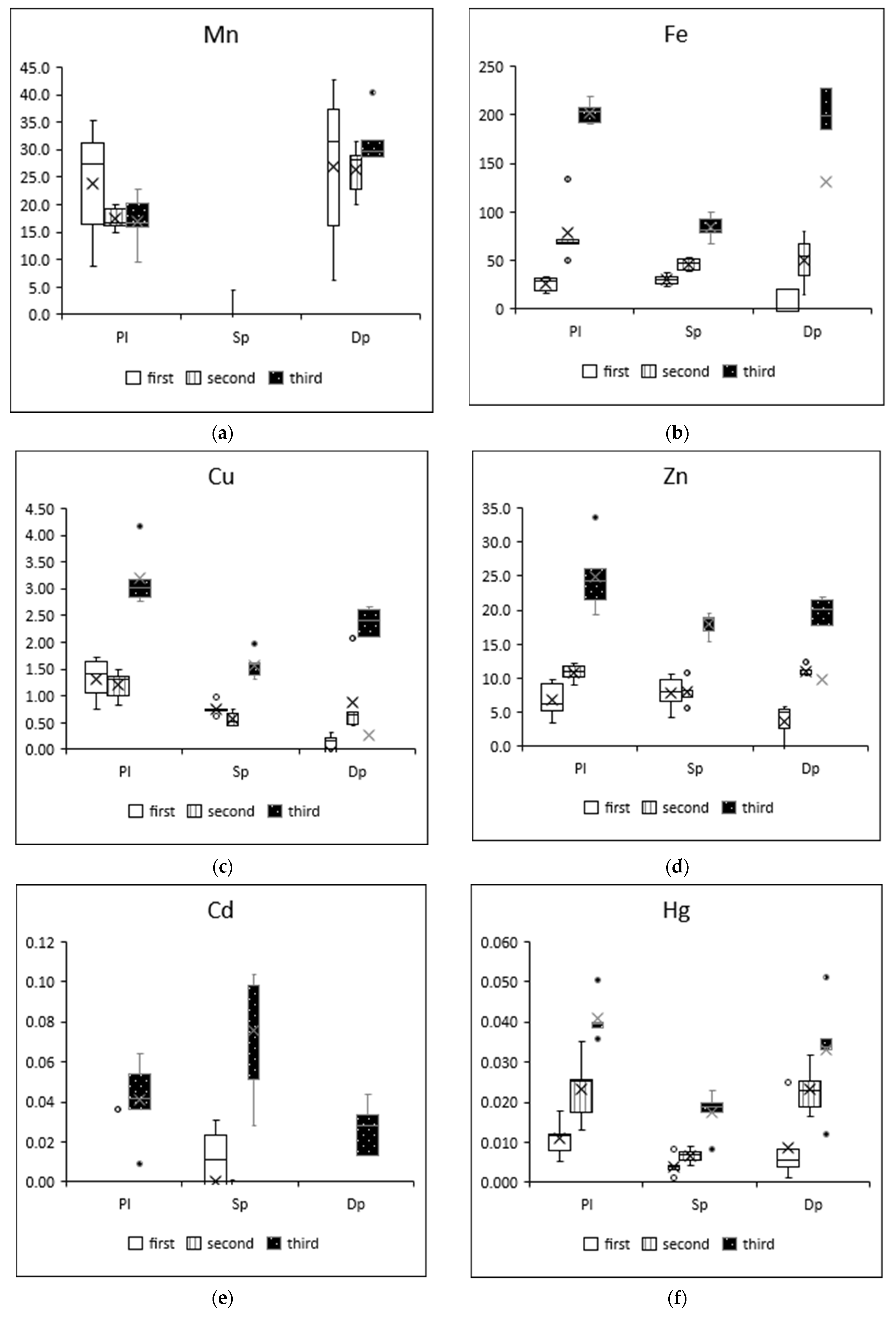
| Mn | Fe | Cu | Zn | Cd | Hg | Pb | |
|---|---|---|---|---|---|---|---|
| 1st month min | 64.1 | 6305 | 202 | 951 | 21.7 | 67.5 | 124 |
| max | 473 | 29,664 | 586 | 4433 | 21.7 | 88.8 | 6049 |
| median | 182 | 11,036 | 327 | 2091 | 21.7 | 81.6 | 2312 |
| average | 189 | 12,033 | 352 | 2215 | 21.7 | 79.3 | 2216 |
| SD | 81.8 | 4613 | 115 | 804 | - | 10.8 | 1442 |
| n | 31 | 31 | 31 | 31 | 1 | 3 | 31 |
| 2nd month min | 93.5 | 6335 | 182 | 1066 | 8.70 | 49.2 | 443 |
| max | 661 | 29,712 | 584 | 6545 | 207 | 69.2 | 5499 |
| median | 213 | 10,138 | 320 | 2240 | 117 | 68.7 | 1892 |
| average | 252 | 11,163 | 357 | 2634 | 103 | 62.4 | 2065 |
| SD | 117 | 4801 | 112 | 1454 | 57.8 | 11.4 | 1159 |
| n | 31 | 31 | 31 | 31 | 31 | 3 | 31 |
| 3rd month min | 8.70 | 3774 | 196 | 691 | 4.35 | 74.5 | 234 |
| max | 247 | 19,722 | 834 | 7184 | 59.8 | 81.0 | 8963 |
| median | 96.7 | 7575 | 358 | 1245 | 35.3 | 78.5 | 1011 |
| average | 110 | 8953 | 432 | 2453 | 34.4 | 78.0 | 1651 |
| SD | 82.7 | 3855 | 183 | 2003 | 20.4 | 3.29 | 2049 |
| n | 15 | 19 | 19 | 19 | 8 | 3 | 19 |
Publisher’s Note: MDPI stays neutral with regard to jurisdictional claims in published maps and institutional affiliations. |
© 2022 by the authors. Licensee MDPI, Basel, Switzerland. This article is an open access article distributed under the terms and conditions of the Creative Commons Attribution (CC BY) license (https://creativecommons.org/licenses/by/4.0/).
Share and Cite
Świsłowski, P.; Nowak, A.; Wacławek, S.; Ziembik, Z.; Rajfur, M. Is Active Moss Biomonitoring Comparable to Air Filter Standard Sampling? Int. J. Environ. Res. Public Health 2022, 19, 4706. https://doi.org/10.3390/ijerph19084706
Świsłowski P, Nowak A, Wacławek S, Ziembik Z, Rajfur M. Is Active Moss Biomonitoring Comparable to Air Filter Standard Sampling? International Journal of Environmental Research and Public Health. 2022; 19(8):4706. https://doi.org/10.3390/ijerph19084706
Chicago/Turabian StyleŚwisłowski, Paweł, Arkadiusz Nowak, Stanisław Wacławek, Zbigniew Ziembik, and Małgorzata Rajfur. 2022. "Is Active Moss Biomonitoring Comparable to Air Filter Standard Sampling?" International Journal of Environmental Research and Public Health 19, no. 8: 4706. https://doi.org/10.3390/ijerph19084706
APA StyleŚwisłowski, P., Nowak, A., Wacławek, S., Ziembik, Z., & Rajfur, M. (2022). Is Active Moss Biomonitoring Comparable to Air Filter Standard Sampling? International Journal of Environmental Research and Public Health, 19(8), 4706. https://doi.org/10.3390/ijerph19084706