
Numerical Investigations of Urban Pollutant Dispersion and Building Intake Fraction with Various 3D Building Configurations and Tree Plantings

 , , and
Abstract
:1. Introduction
2. Methodology
2.1. Definition of Crucial Parameters
2.1.1. Velocity Ratio (VR)
2.1.2. Building Intake Fraction <P_IF>
2.2. Set-Up for Numerical Modelling
2.2.1. CFD Model Description
2.2.2. Model Set-Up and Boundary Conditions
2.2.3. Description of Pollutant Dispersion Modelling
2.2.4. Description of the Vegetation Modelling
2.2.5. Validations for Flow, Dispersion and Vegetation Modelling
- Flow validation by wind tunnel tests of cubic arrays
- Pollutant dispersion validation by wind tunnel tests without tree models
- Pollutant dispersion validation by wind tunnel tests with tree models
3. Results
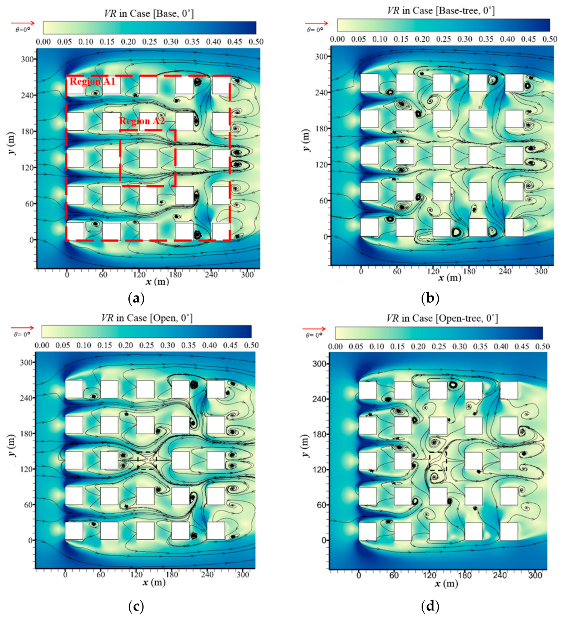
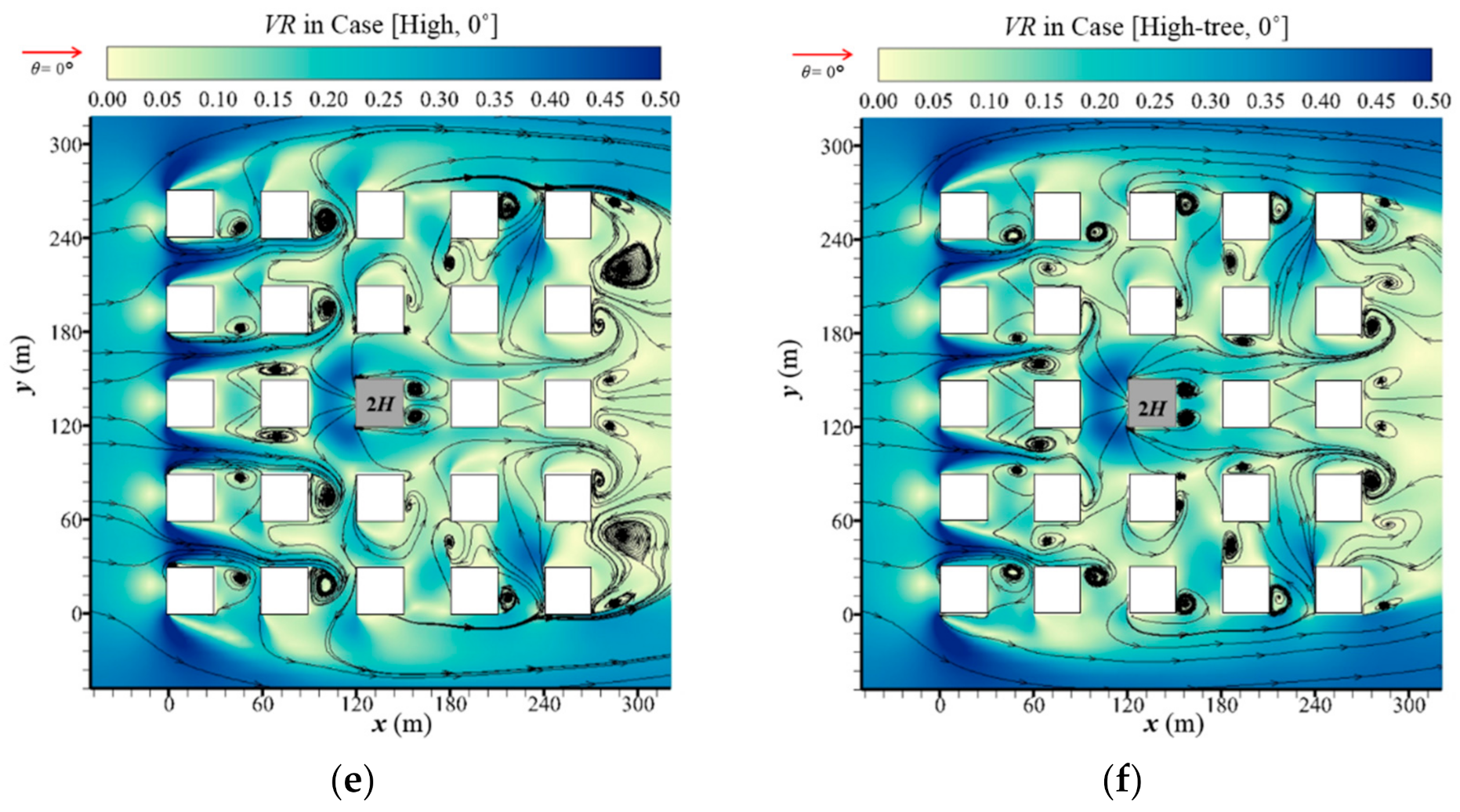
3.1. Impacts of Building Configurations and Tree Planting on Flow Pattern
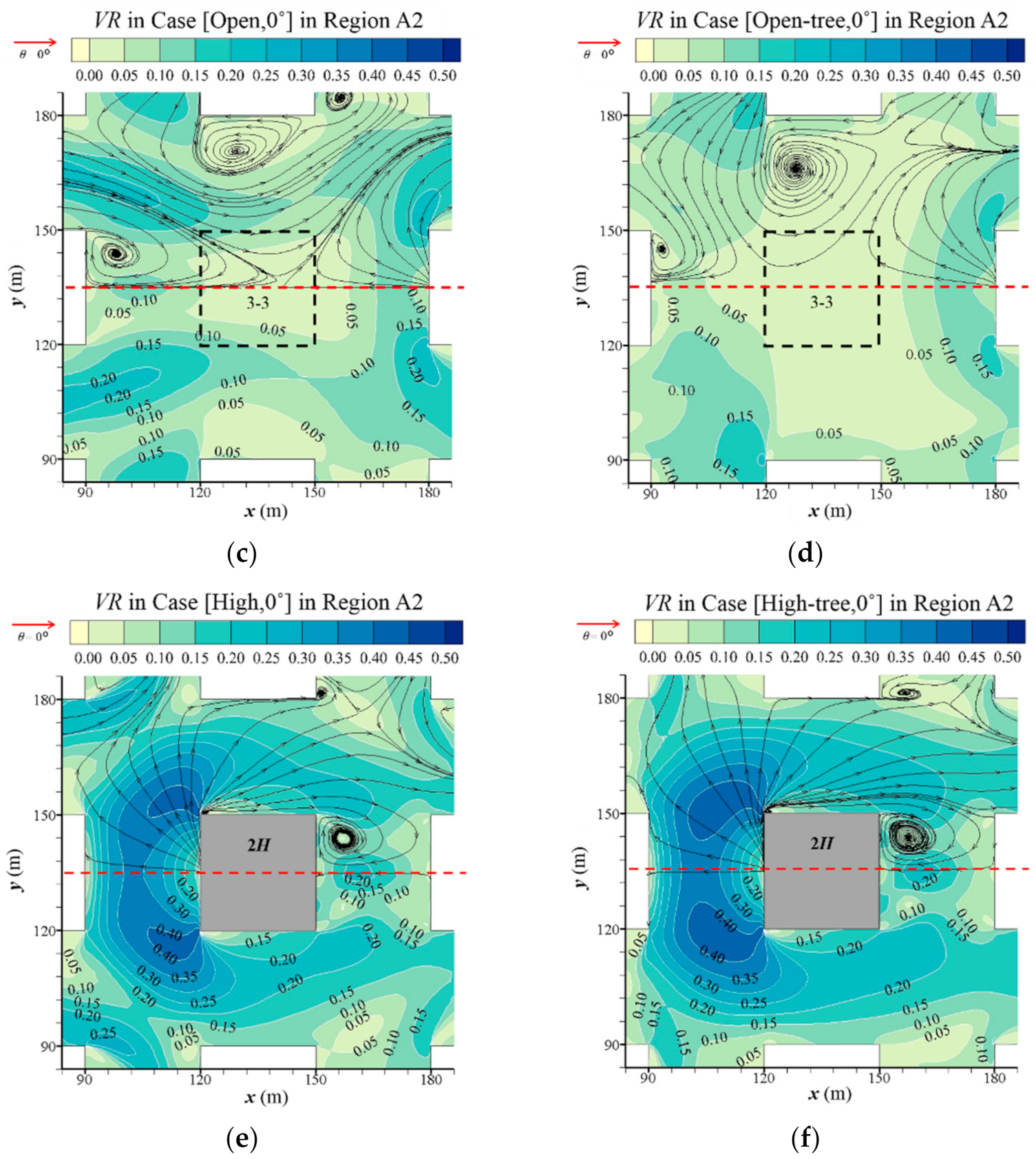
3.1.1. Impact of Open Space and High-Rise Building on Airflow
3.1.2. Influence of Tree Planting on Airflow
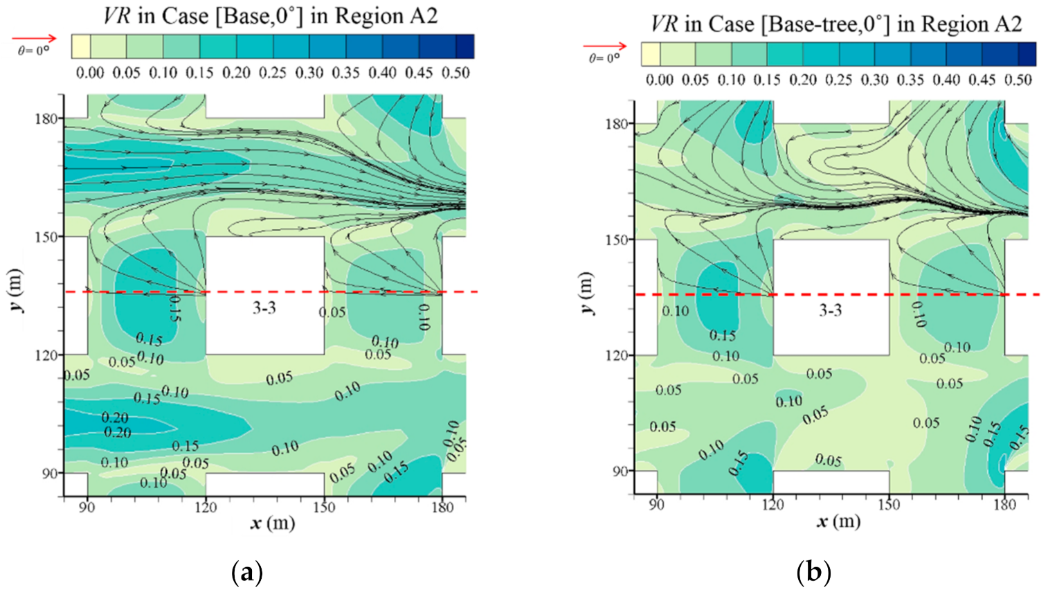
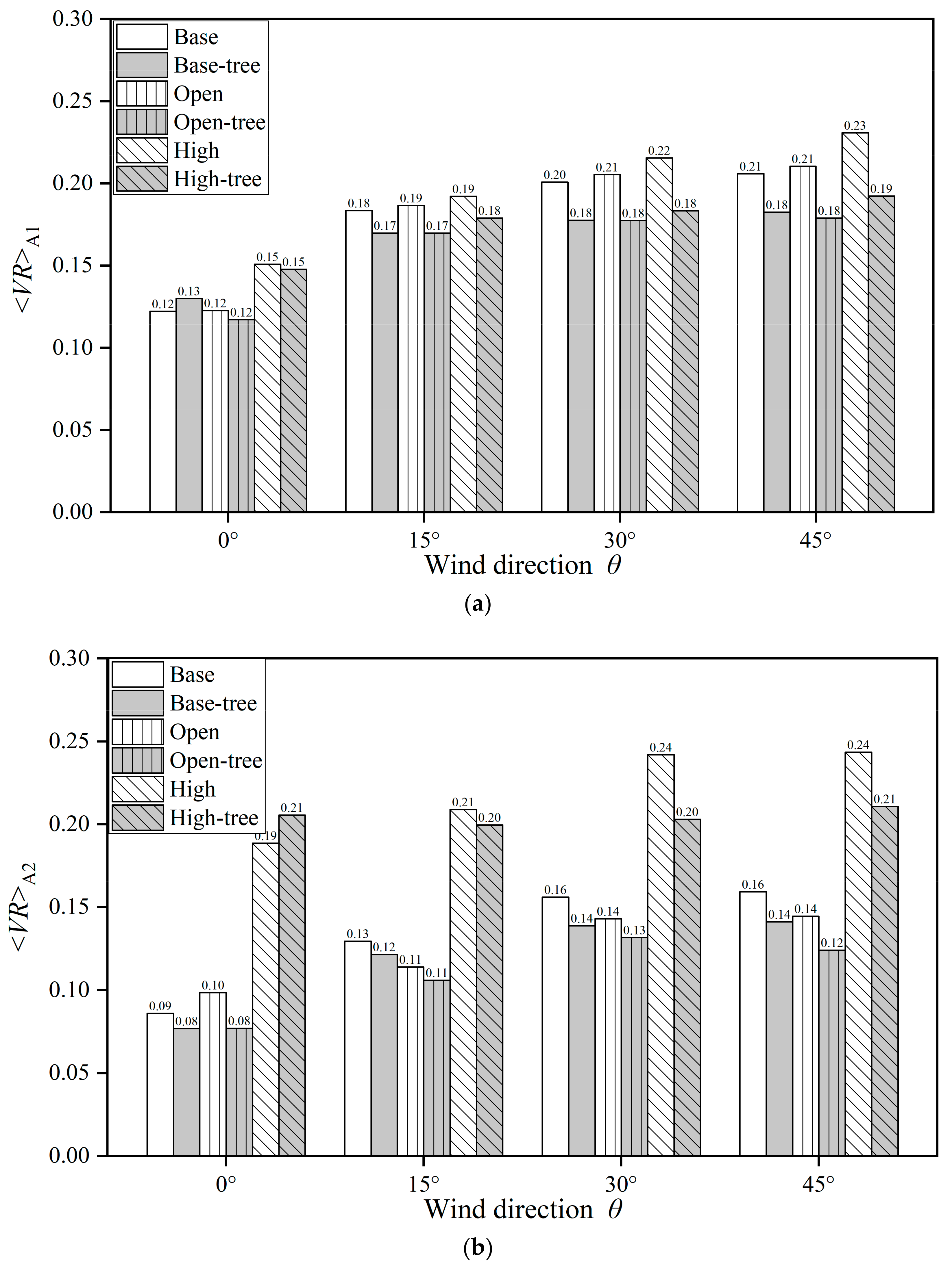
3.1.3. Quantitative Analysis of Impact of Different Urban Layouts on Velocity Field
3.2. Impacts of Building Configurations and Tree Planting on Pollutant Dispersion
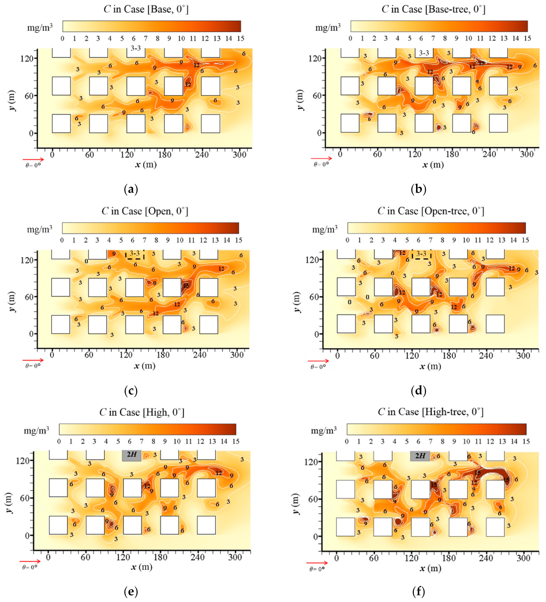
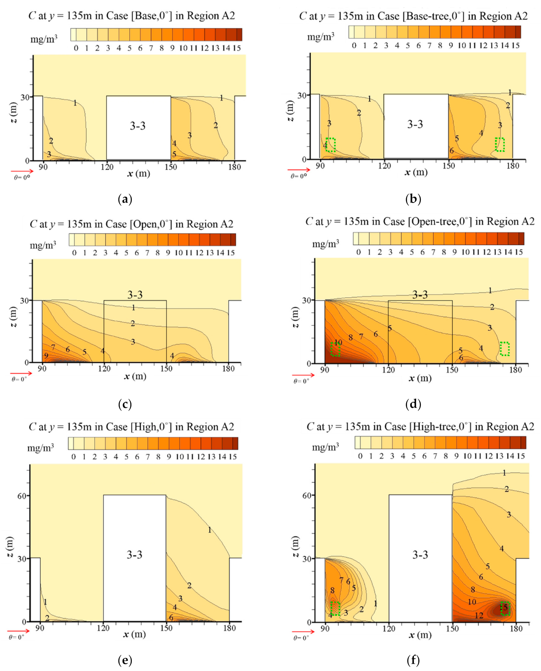
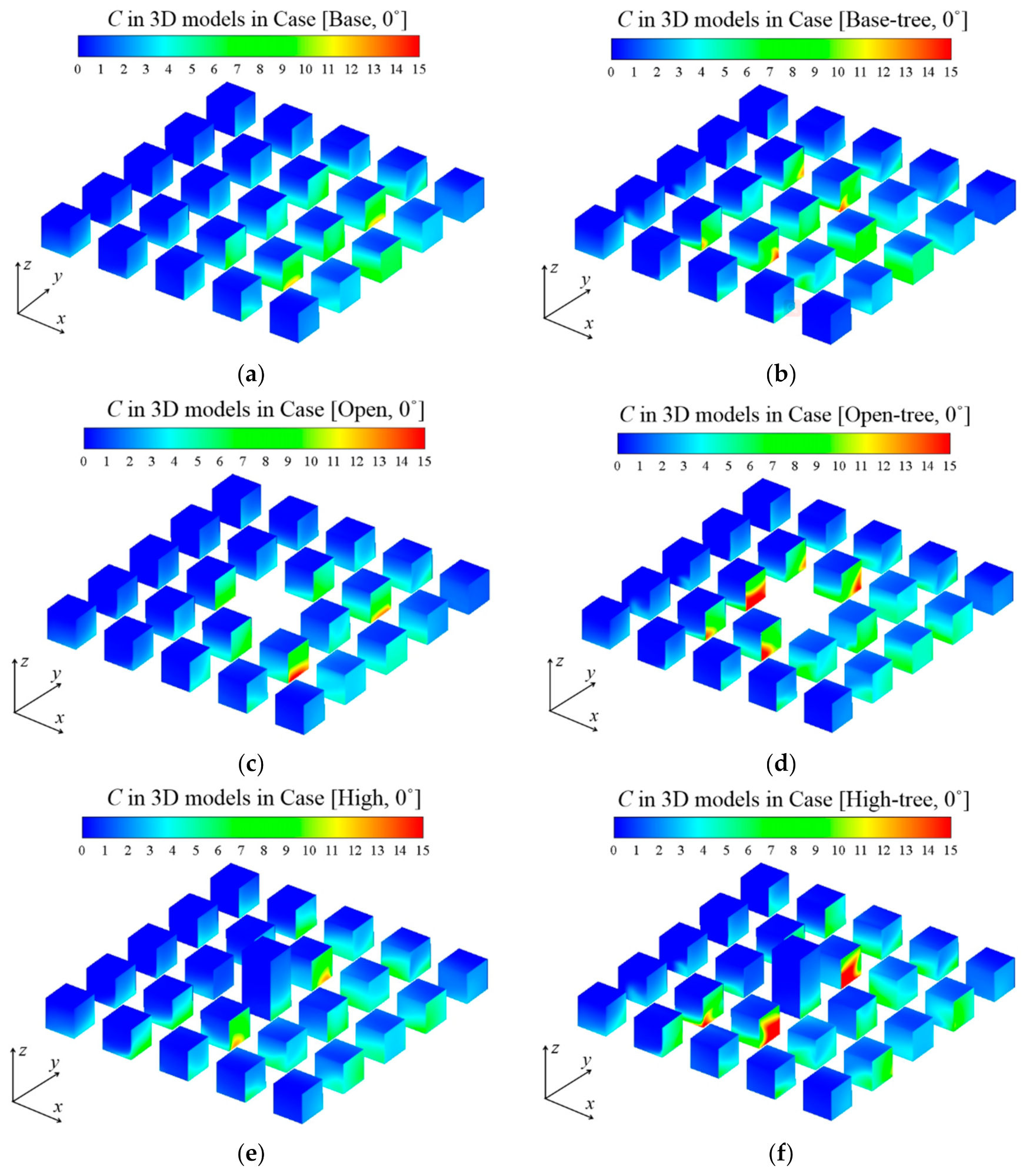
3.2.1. Influence of Open Space and High-Rise Building on Pollutant Dispersion
3.2.2. Influence of Tree Planting on Pollutant Dispersion
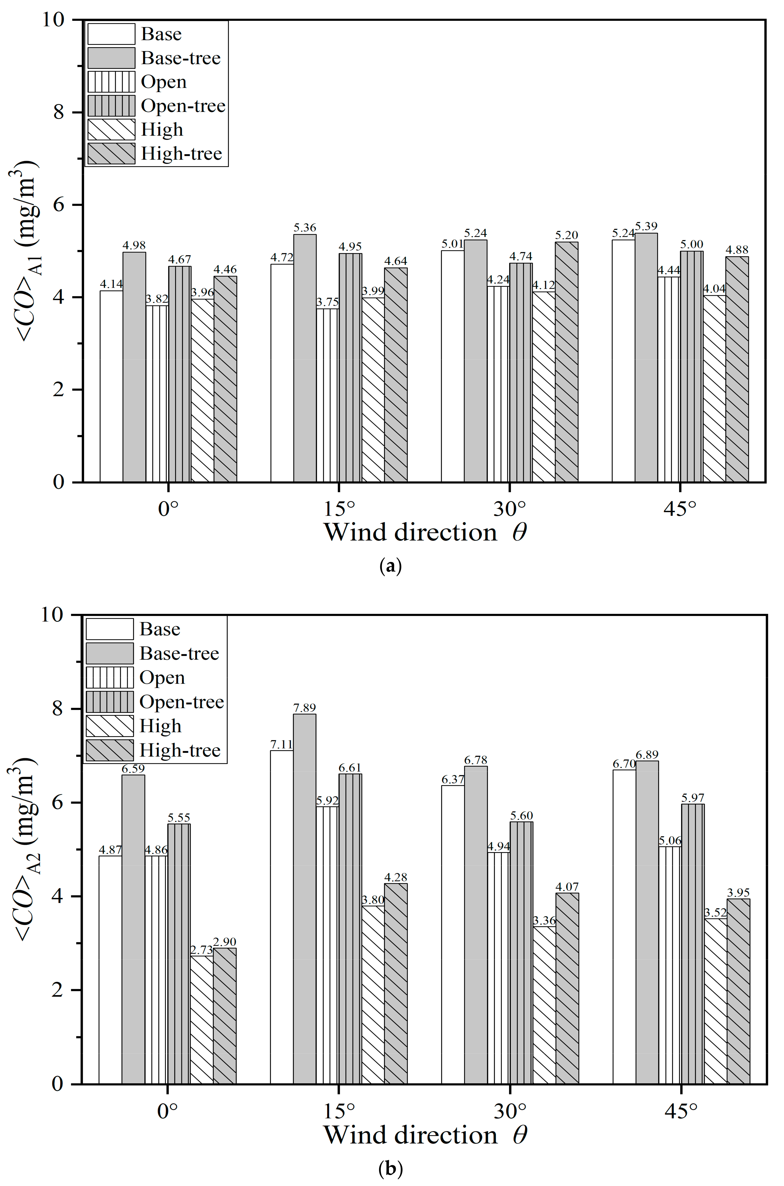
3.2.3. Quantitative Analysis for Impact of Building Configurations and Tree Planting on Pollutant Dispersion
3.3. Impacts of Building Configurations and Tree Planting on <P_IF>
3.4. Velocity, CO Concentration and <P_IF> in Surrounding Area of A2 (Region A1−A2)
4. Discussion
5. Conclusions
- (1)
- Without tree planting, in contrast to the general 5 × 5 uniform-height building cluster (H = B = W = 30m), open space (the central building is removed) increases the spatially-averaged velocity ratio (VR) for the whole urban area under all four approaching wind directions (0°, 15°, 30° and 45°) by 0.40–2.27%. Designing the central building to be taller (2H) than the surroundings (H) can increase the VR for the entire urban area by 4.73–23.36%. In particular, the mean wind speed at the pedestrian level (z = 2 m) in the area around the high-rise building is significantly increased by 52.78–119.05%. However, tree planting significantly decreases the urban wind speed at z = 2 m on the basis of either open space or high-rise building designs, by 4.63–14.99% or 2.04–16.68%, respectively.
- (2)
- Pollutant dispersion is determined by urban airflow characteristics. CO is released near the ground as a surrogate of traffic emissions. Without tree planting, both open space and central high-rise building would decrease the mean C at the pedestrian level for the whole urban area by 7.83–20.54% (0.32–0.97 mg/m3) and 4.39–23.00% (0.18–1.2 mg/m3) separately. This decreasing effect on C is significantly stronger for the high-rise building in the central area, by 43.88–47.40% (2.14–3.18 mg/m3). On the contrary, urban tree planting evidently weakens the pollutant dilution in all scenarios, with the increasing rate of 2.84–31.88% (0.15–1.2 mg/m3) for C at the pedestrian level in the entire urban area.
- (3)
- The traffic-related CO exposure on residents in kerbside buildings is evaluated by <P_IF>. For the tree-free scenarios, both open space and high-rise buildings could decrease <P_IF> with the wind from all four directions by 6.56–16.08% and 9.59–24.70%, respectively. In contrast, tree planting obviously increases personal exposure in all scenarios by 14.89–50.19%. The <P_IF> of the tree-free cases ranges from 1.54 to 2.53 ppm, while <P_IF> ranges from 2.05 to 2.90 ppm in cases with tree planting.
Author Contributions
Funding
Conflicts of Interest
Nomenclature
| AR, H/W | aspect ratio |
| B, H, W | building width, building height and street width (m) |
| Br | volume-mean breathing rate (m3/s) |
| C | time-averaged pollutant (CO) concentration (kg/m3) |
| Cd | leaf drag coefficient |
| <CO>A1, <CO>A2 | the spatial mean CO concentration at z = 2 m in Region A1 and in Region A2 (mg/m3) |
| Dm, Dt | molecular and turbulent diffusivity of the pollutant (m2/s) |
| I/O | indoor/outdoor pollutant concentration ratio |
| IF | intake fraction |
| k, ε | turbulent kinetic energy (m2/s2) and its dissipation rate (m2/s3) |
| LAD | leaf area density (m2/m3) |
| m | total pollutant emission over the considered period (kg) |
| M, N | total number of micro-environment types and population age groups |
| P | number of the population |
| P_IF, <P_IF> | personal intake fraction (ppm), building intake fraction (ppm) |
| Re | Reynolds number |
| S | realistic CO emission rate (kg/m3/s) |
| SCt | turbulent Schmidt number |
| , Sk, Sε | additional source and sink terms of momentum, k and ε (kg/m/s3) |
| t | time (s) |
| time-averaged velocity component (m/s) on stream-wise (), span-wise (, lateral) and vertical () directions, as j = 1, 2, 3 | |
| U | velocity magnitude (m/s) |
| Uin(z) | velocity profiles used at CFD domain inlet (m/s) |
| Uref, u* | reference velocity at building height and friction velocity (m/s) |
| v, vt | kinematic viscosity and kinetic eddy viscosity (m2/s) |
| Vp, Vδ | wind velocity at pedestrian-level and at the top of boundary layer (m/s) |
| VR | velocity ratio |
| <VR>A1, <VR>A2 | the spatial mean velocity ratio at z = 2 m in Region A1 and in Region A2 (mg/m3) |
| xj | spatial coordinates (m) on stream-wise (x), span-wise (y) and vertical (z) directions, as j = 1, 2, 3 |
| βd | portion of turbulent kinetic energy converted from mean kinetic energy under the influence of drag |
| βp | dimensionless coefficient of the Kolmogorov cascade |
| θ | wind direction (°) |
| κv | von Kármán constant |
| λp, λf | building plan area density, frontal area density |
| ρ | air density (kg/m3) |
Appendix A
- Factors for exposure assessmentTable A1. Population composition and related factors for exposure assessment.
Item Juveniles Adults Elderly Percentage of total population 21.2% 63.3% 15.5% Breathing rate Br indoors at home (m3/day) 12.5 13.8 13.1 Time spent indoors at home (percentage) 61.70% 59.50% 71.60% - Validation studies for the flow, dispersion and vegetation modelling
- 2.1.
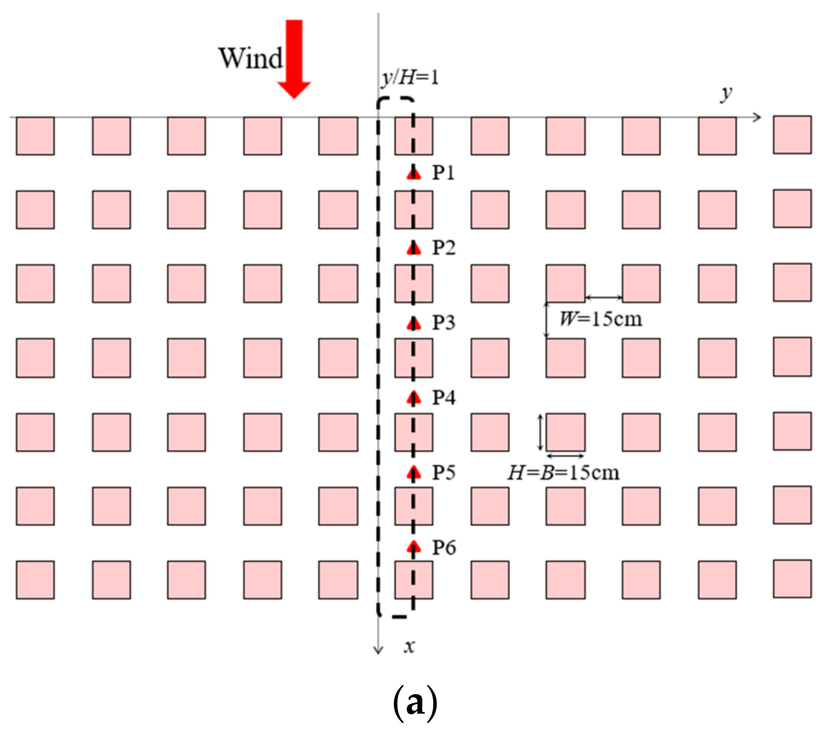
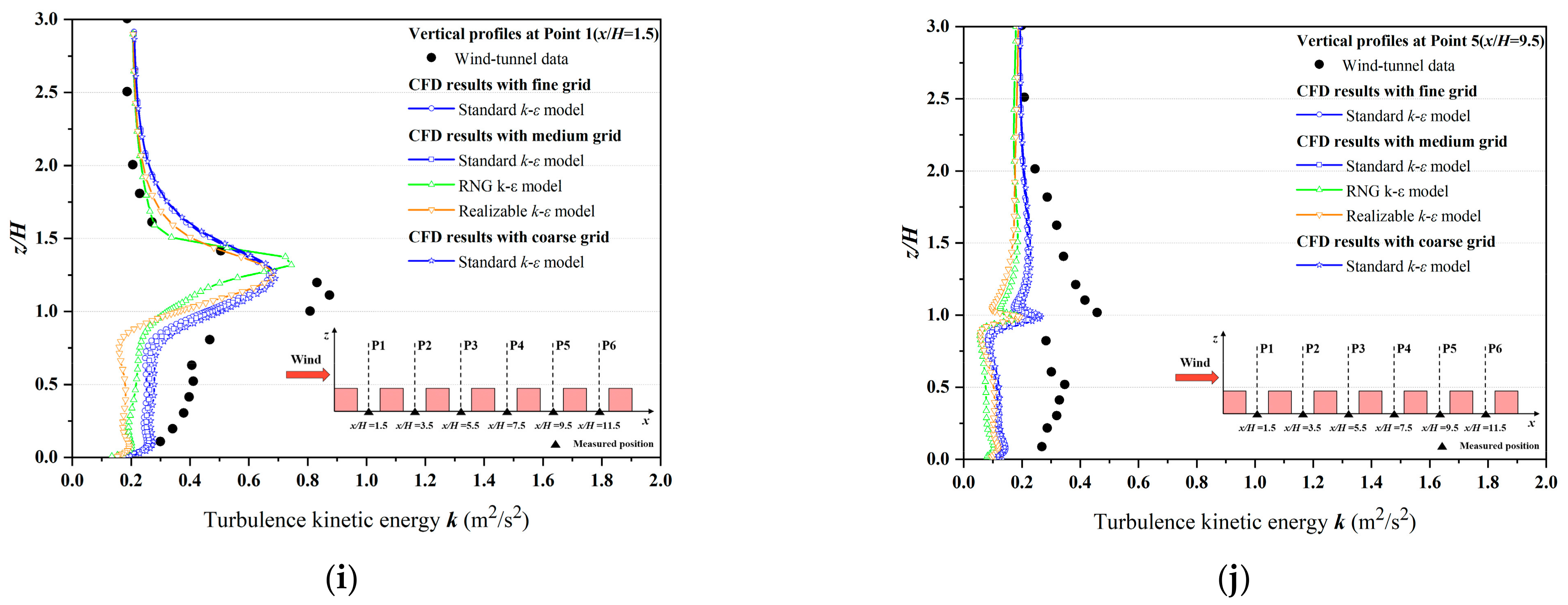
- CFD validation of flow modellingFigure A1. Flow validation by wind tunnel data. (a) Geometry of the UCL model in wind tunnel dataset. (b) Setting of the computational domain and boundary conditions. (c–h) Vertical profiles of monitored and modelled stream-wise velocity () at Point P1–P6. (i,j) Vertical profiles of monitored and modelled turbulence kinetic energy (k) at Point P1 and P5.Figure A1. Flow validation by wind tunnel data. (a) Geometry of the UCL model in wind tunnel dataset. (b) Setting of the computational domain and boundary conditions. (c–h) Vertical profiles of monitored and modelled stream-wise velocity () at Point P1–P6. (i,j) Vertical profiles of monitored and modelled turbulence kinetic energy (k) at Point P1 and P5.
![Ijerph 19 03524 g0a1a]()
![Ijerph 19 03524 g0a1b]()
![Ijerph 19 03524 g0a1c]() Table A2. Statistical analysis between wind tunnel data and CFD simulation results—flow validation.
Table A2. Statistical analysis between wind tunnel data and CFD simulation results—flow validation.Variable (Position) Grid Size Turbulence Model NMSE * FB ** R *** Criteria ≤1.5 −0.3–0.3 → 1.0 Stream-wise velocity at P1 Fine grid STD 0.054 0.084 0.990 Medium grid STD 0.049 0.087 0.990 RNG 0.107 0.018 0.996 RKE 0.115 0.094 0.986 Coarse grid STD 0.038 0.081 0.991 Stream-wise velocity at P2 Fine grid STD 0.007 0.002 0.999 Medium grid STD 0.009 0.002 0.997 RNG 0.045 −0.090 0.994 RKE 0.016 −0.083 0.998 Coarse grid STD 0.011 0.013 0.997 Stream-wise velocity at P3 Fine grid STD 0.012 −0.063 0.996 Medium grid STD 0.005 −0.024 0.998 RNG 0.093 −0.179 0.996 RKE 0.022 −0.100 0.997 Coarse grid STD 0.005 −0.013 0.997 Stream-wise velocity at P4 Fine grid STD 0.014 −0.057 0.999 Medium grid STD 0.014 −0.034 1.000 RNG 0.053 −0.175 0.998 RKE 0.014 −0.102 0.999 Coarse grid STD 0.015 −0.023 0.999 Stream-wise velocity at P5 Fine grid STD 0.019 −0.051 0.998 Medium grid STD 0.021 −0.017 0.998 RNG 0.033 −0.130 0.998 RKE 0.016 −0.073 0.997 Coarse grid STD 0.022 −0.009 0.997 Stream-wise velocity at P6 Fine grid STD 0.037 −0.104 0.995 Medium grid STD 0.037 −0.058 0.997 RNG 0.039 −0.147 0.993 RKE 0.039 −0.106 0.993 Coarse grid STD 0.035 −0.048 0.998 TKE at P1 Fine grid STD 0.137 0.177 0.820 Medium grid STD 0.115 0.150 0.842 RNG 0.275 0.343 0.662 RKE 0.361 0.366 0.727 Coarse grid STD 0.091 0.115 0.867 TKE at P5 Fine grid STD 0.610 0.615 0.076 Medium grid STD 0.621 0.615 0.135 RNG 1.299 0.837 −0.105 RKE 1.096 0.802 −0.378 Coarse grid STD 0.526 0.575 0.255 * normalised mean square error. ** fractional bias-. *** correlation coefficient–. - 2.2.
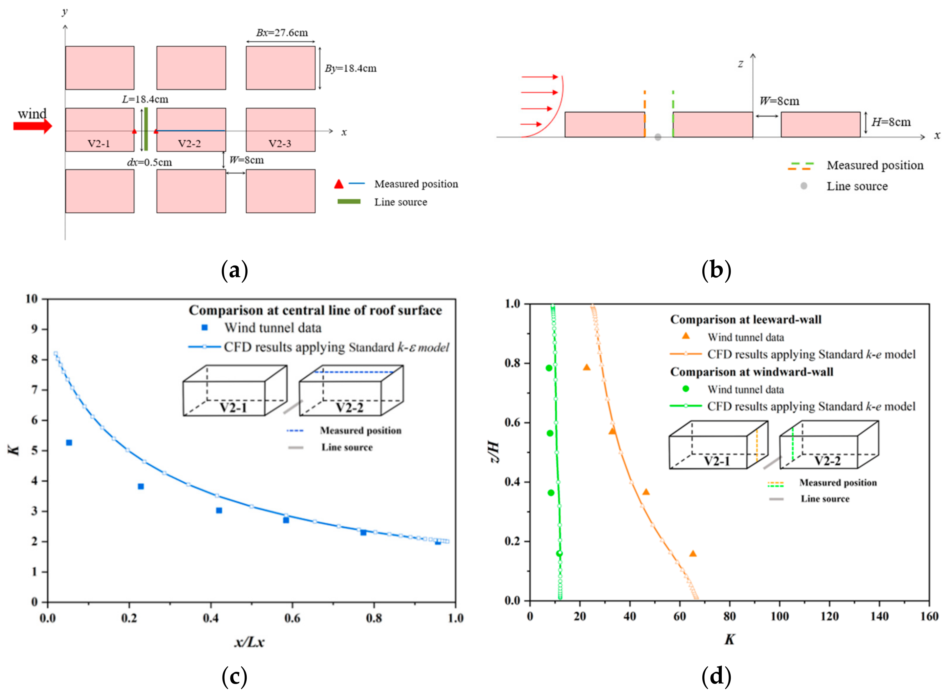
- CFD validation of pollutant dispersion without tree modelsFigure A2. Validation for pollutant dispersion. (a) Configurations of the wind tunnel experiment with top view. (b) Configurations of the wind tunnel experiment with lateral view. (c) Vertical profiles of normalized inert gas concentration K at the roof top of the model. (d) Vertical profiles of K at the leeward and windward wall.Figure A2. Validation for pollutant dispersion. (a) Configurations of the wind tunnel experiment with top view. (b) Configurations of the wind tunnel experiment with lateral view. (c) Vertical profiles of normalized inert gas concentration K at the roof top of the model. (d) Vertical profiles of K at the leeward and windward wall.
![Ijerph 19 03524 g0a2]() Table A3. Statistical analysis between wind tunnel data and CFD simulation results—dispersion modelling.Table A3. Statistical analysis between wind tunnel data and CFD simulation results—dispersion modelling.
Table A3. Statistical analysis between wind tunnel data and CFD simulation results—dispersion modelling.Table A3. Statistical analysis between wind tunnel data and CFD simulation results—dispersion modelling.Variable (Position) NMSE * FB ** R *** Criteria ≤1.5 −0.3–0.3 → 1.0 Leeward wall 0.021 −0.012 0.997 Windward wall 0.064 −0.223 0.855 Central line 0.029 −0.13 0.998 * normalised mean square error: . ** fractional bias-. *** correlation coefficient–. - 2.3.
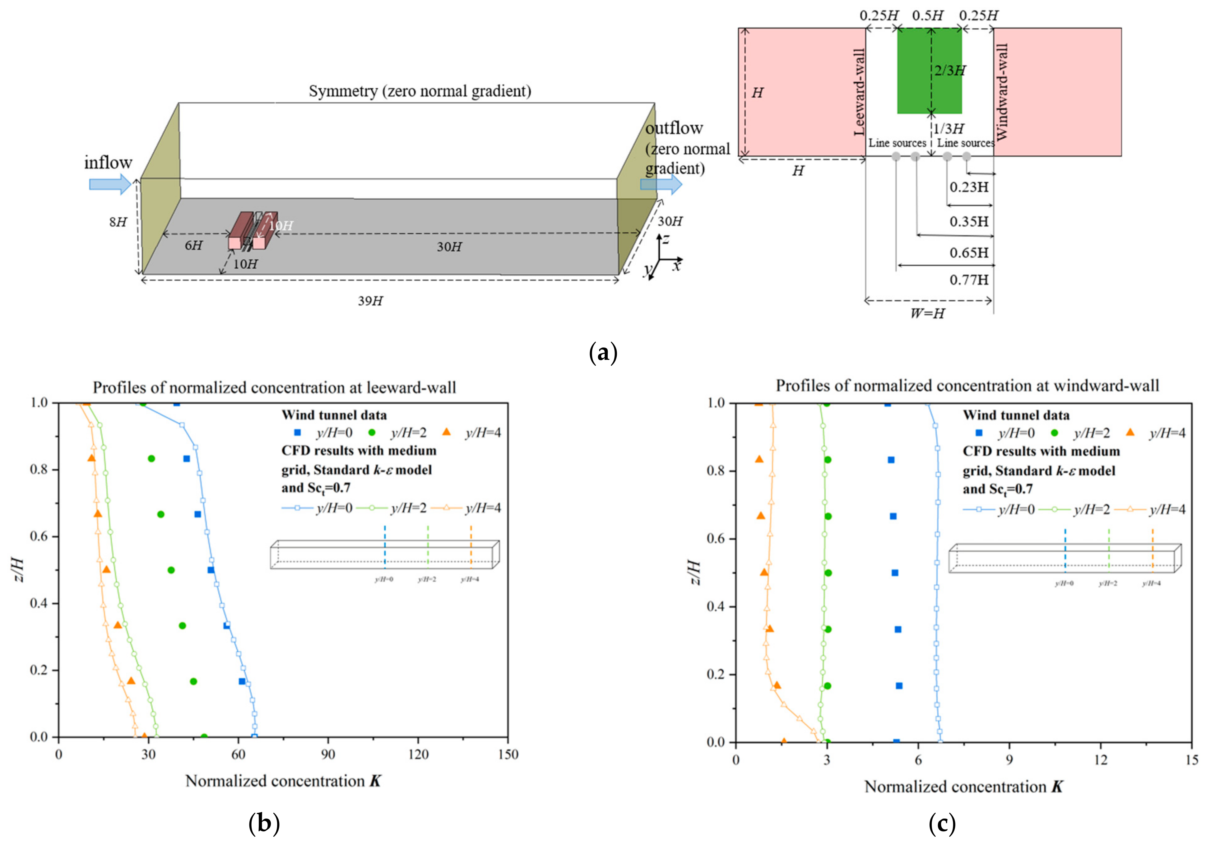
- CFD validation of pollutant dispersion with tree modelsFigure A3. Validation for the vegetation modelling. (a) Configurations of the wind tunnel experiment with vegetation model. (b) Vertical profiles of K at the leeward wall. (c) Vertical profiles of K at the windward wall.Figure A3. Validation for the vegetation modelling. (a) Configurations of the wind tunnel experiment with vegetation model. (b) Vertical profiles of K at the leeward wall. (c) Vertical profiles of K at the windward wall.
![Ijerph 19 03524 g0a3]() Table A4. Statistical analysis between wind tunnel data and CFD simulation results—vegetation modelling.Table A4. Statistical analysis between wind tunnel data and CFD simulation results—vegetation modelling.
Table A4. Statistical analysis between wind tunnel data and CFD simulation results—vegetation modelling.Table A4. Statistical analysis between wind tunnel data and CFD simulation results—vegetation modelling.Variable (Position) NMSE * FB ** R *** Criteria ≤1.5 −0.3–0.3 → 1.0 Leeward side y/H = 0 0.159 0.011 0.918 y/H = 2 1.306 0.594 0.987 y/H = 4 0.108 0.128 0.974 Windward side y/H = 0 0.055 −0.233 0.630 y/H = 2 0.007 0.049 0.784 y/H = 4 0.221 −0.256 0.700 * normalised mean square error: . ** fractional bias-. *** correlation coefficient–.
- Quantitative investigations of the flow, pollutant concentration and traffic-related exposureTable A5. Spatial mean velocity ratio (VR) at z = 2 m in Region A1 (<VR>A1) and Region A2 (<VR>A2) of each scenario and the change rate.Table A5. Spatial mean velocity ratio (VR) at z = 2 m in Region A1 (<VR>A1) and Region A2 (<VR>A2) of each scenario and the change rate.
Case <VR>A1 <VR>A2 0° 15° 30° 45° 0° 15° 30° 45° Case [Base] 0.12 0.18 0.20 0.21 0.09 0.13 0.16 0.16 Case [Open] 0.12 0.19 0.21 0.21 0.10 0.11 0.14 0.14 +0.40% +1.70% +2.27% +2.22% +14.53% −12.06% −8.40% −9.29% Case [High] 0.15 0.19 0.22 0.23 0.19 0.21 0.24 0.24 +23.36% +4.73% +7.30% +12.07% +119.05% +61.30% +55.06% +52.78% Case [Base-tree] 0.13 0.17 0.18 0.18 0.08 0.12 0.14 0.14 +6.27% −7.51% −11.59% −11.41% −10.76% −6.22% −11.08% −11.43% Case [Open-tree] 0.12 0.17 0.18 0.18 0.08 0.11 0.13 0.12 −4.63% −9.01% −13.65% −14.99% −21.92% −6.91% −7.84% −14.18% Case [High-tree] 0.15 0.18 0.18 0.19 0.21 0.20 0.20 0.21 −2.04% −6.87% −14.93% −16.68% +8.98% −4.42% −16.11% −13.44% The percentage number in each cell denotes the change rate of each case. Case [Base] is the comparison reference for Case [Open], Case [High] and Case [Base-tree]. The change rate of Case [Open-tree] refers to Case [Open], and that of Case [High-tree] refers to Case [High].Table A6. Spatial mean CO concentration (C) at z = 2 m in Region A1 (<CO>A1) and Region A2 (<CO>A2) of each scenario and the change rate.Table A6. Spatial mean CO concentration (C) at z = 2 m in Region A1 (<CO>A1) and Region A2 (<CO>A2) of each scenario and the change rate.Case <CO>A1 (mg/m3) <CO>A2 (mg/m3) 0° 15° 30° 45° 0° 15° 30° 45° Case [Base] 4.14 4.72 5.01 5.24 4.87 7.11 6.37 6.70 Case [Open] 3.82 3.75 4.24 4.44 4.86 5.92 4.94 5.06 −7.83% −20.54% −15.31% −15.27% −0.08% −16.82% −22.48% −24.43% Case [High] 3.96 3.99 4.12 4.04 2.73 3.80 3.36 3.52 −4.39% −15.47% −17.78% −23.00% −43.88% −46.58% −47.24% −47.40% Case [Base-tree] 4.98 5.36 5.24 5.39 6.59 7.89 6.78 6.89 +20.19% +13.55% +4.73% +2.84% +35.46% +10.93% +6.47% +2.85% Case [Open-tree] 4.67 4.95 4.74 5.00 5.55 6.61 5.60 5.97 +22.44% +31.88% +11.80% +12.64% +14.09% +11.76% +13.35% +17.93% Case [High-tree] 4.46 4.64 5.20 4.88 2.90 4.28 4.07 3.95 +12.61% +16.31% +26.38% +20.88% +6.10% +12.57% +21.19% +12.04% The percentage data denote the change rate of each case in contrast to Case [Base]. The change rate of Case [Open-tree] refers to Case [Open], and that of Case [High-tree] refers to Case [High].Table A7. Building intake fraction <P_IF> and the change rate in different cases.Case <P_IF> (ppm) 0° 15° 30° 45° Case [Base] 1.71 2.23 2.32 2.53 Case [Open] 1.59 1.87 2.05 2.19 −6.56% −16.08% −11.65% −13.19% Case [High] 1.54 1.89 1.86 1.90 −9.59% −15.00% −19.74% −24.70% Case [Base-tree] 2.05 2.87 2.75 2.90 +19.94% +28.92% +18.24% +14.89% Case [Open-tree] 2.00 2.65 2.51 2.68 +25.67% +41.62% +22.22% +22.43% Case [High-tree] 2.32 2.41 2.57 2.48 +50.19% +27.28% +37.63% +30.51% The percentage number in each cell denotes the rate of change of each case. Case [Base] is the comparison reference for Case [Open], Case [High] and Case [Base-tree]. The change rate of Case [Open-tree] refers to Case [Open], and that of Case [High-tree] refers to Case [High].Table A8. Spatial mean velocity ratio (VR) at z = 2 m in the Region A1−A2 (<VR>A1−A2) of each scenario and the change rate.Table A8. Spatial mean velocity ratio (VR) at z = 2 m in the Region A1−A2 (<VR>A1−A2) of each scenario and the change rate.Case Name <VR>A1−A2 0° 15° 30° 45° Case [Base] 0.55 0.83 0.90 0.92 Case [Open] 0.59 0.76 0.79 0.81 +7.71% −7.61% −11.64% −11.41% Case [High] 0.55 0.85 0.93 0.95 −7.90% +11.35% +16.88% +16.60% Case [Base-tree] 0.53 0.77 0.79 0.81 −2.94% −9.16% −14.14% −15.06% Case [Open-tree] 0.63 0.83 0.92 0.99 +19.69% +6.92% +15.91% +23.36% Case [High-tree] 0.61 0.77 0.79 0.82 −3.82% −7.20% −14.76% −17.11% The percentage number in each cell denotes the rate of change of each case. Case [Base] is the comparison reference for Case [Open], Case [High] and Case [Base-tree]. The change rate of Case [Open-tree] refers to Case [Open], and that of Case [High-tree] refers to Case [High].Table A9. Spatial mean CO concentration (C) at z = 2 m in the Region A1−A2 (<CO>A1−A2) of each scenario and the change rate.Table A9. Spatial mean CO concentration (C) at z = 2 m in the Region A1−A2 (<CO>A1−A2) of each scenario and the change rate.Case Name <CO>A1−A2 0° 15° 30° 45° Case [Base] 4.05 4.42 4.84 5.06 Case [Open] 4.78 5.04 5.05 5.20 +17.89% +14.07% +4.45% +2.83% Case [High] 3.69 3.48 4.15 4.36 −22.81% −31.00% −17.79% −16.13% Case [Base-tree] 4.56 4.74 4.63 4.88 +23.82% +36.15% +11.57% +11.87% Case [Open-tree] 4.11 4.01 4.21 4.10 −9.88% −15.29% −9.13% −16.01% Case [High-tree] 4.65 4.69 5.34 5.00 +13.15% +16.75% +26.89% +21.83% The percentage number in each cell denotes the rate of change of each case. Case [Base] is the comparison reference for Case [Open], Case [High] and Case [Base-tree]. The change rate of Case [Open-tree] refers to Case [Open], and that of Case [High-tree] refers to Case [High].


References
- Chan, C.K.; Yao, X. Air pollution in mega cities in China. Atmos. Environ. 2008, 42, 1–42. [Google Scholar] [CrossRef]
- Fenger, J. Urban air quality. Atmos. Environ. 1999, 33, 4877–4900. [Google Scholar] [CrossRef]
- Pu, Y.; Yang, C. Estimating urban roadside emissions with an atmospheric dispersion model based on in-field measurements. Environ. Pollut. 2014, 192, 300–307. [Google Scholar] [CrossRef] [PubMed]
- Ji, W.; Zhao, B. Estimating mortality derived from indoor exposure to particles of outdoor origin. PLoS ONE 2015, 10, e0124238. [Google Scholar] [CrossRef] [PubMed] [Green Version]
- Peters, A.; Pope III, C.A. Cardiopulmonary mortality and air pollution. Lancet 2002, 360, 1184–1185. [Google Scholar] [CrossRef]
- Chen, C.; Zhao, B.; Zhou, W.; Jiang, X.; Tan, Z. A methodology for predicting particle penetration factor through cracks of windows and doors for actual engineering application. Build. Environ. 2012, 47, 339–348. [Google Scholar] [CrossRef]
- Quang, T.N.; He, C.; Morawska, L.; Knibbs, L.D.; Falk, M. Vertical particle concentration profiles around urban office buildings. Atmos. Chem. Phys. Discuss. 2012, 12, 5017–5030. [Google Scholar] [CrossRef] [Green Version]
- Zaeh, S.E.; Koehler, K.; Eakin, M.N.; Wohn, C.; Diibor, I.; Eckmann, T.; Wu, T.D.; Clemons-Erby, D.; Gummerson, C.E.; Green, T.; et al. Indoor air quality prior to and following school building renovation in a mid-Atlantic school district. Int. J. Environ. Res. Public Health 2021, 18, 12149. [Google Scholar] [CrossRef]
- Bady, M.; Kato, S.; Huang, H. Towards the application of indoor ventilation efficiency indices to evaluate the air quality of urban areas. Build. Environ. 2008, 43, 1991–2004. [Google Scholar] [CrossRef]
- Ng, W.-Y.; Chau, C.-K. A modeling investigation of the impact of street and building configurations on personal air pollutant exposure in isolated deep urban canyons. Sci. Total Environ. 2014, 468, 429–448. [Google Scholar] [CrossRef]
- Ng, E. Policies and technical guidelines for urban planning of high-density cities-air ventilation assessment (ava) of Hong Kong. Build. Environ. 2009, 44, 1478–1488. [Google Scholar] [CrossRef] [PubMed]
- Chang, C.H.; Meroney, R.N. Concentration and flow distributions in urban street canyons: Wind tunnel and computational data. J. Wind. Eng. Ind. Aerodyn. 2003, 91, 1141–1154. [Google Scholar] [CrossRef]
- Chew, L.W.; Aliabadi, A.A.; Norford, L.K. Flows across high aspect ratio street canyons: Reynolds number independence revisited. Environ. Fluid Mech. 2018, 18, 1275–1291. [Google Scholar] [CrossRef]
- Grimmond, C.; Roth, M.; Oke, T.R.; Au, Y.; Best, M.; Betts, R.; Carmichael, G.; Cleugh, H.; Dabberdt, W.; Emmanuel, R. Climate and more sustainable cities: Climate information for improved planning and management of cities (producers/capabilities perspective). Procedia Environ. Sci. 2010, 1, 247–274. [Google Scholar] [CrossRef] [Green Version]
- Li, X.-X.; Liu, C.-H.; Leung, D.Y.C.; Lam, K.M. Recent progress in CFD modelling of wind field and pollutant transport in street canyons. Atmos. Environ. 2006, 40, 5640–5658. [Google Scholar] [CrossRef]
- Peng, Y.L.; Buccolieri, R.; Gao, Z.; Ding, W. Indices employed for the assessment of “urban outdoor ventilation”—A review. Atmos. Environ. 2020, 223, 117211. [Google Scholar] [CrossRef]
- Tominaga, Y.; Stathopoulos, T. CFD simulation of near-field pollutant dispersion in the urban environment: A review of current modeling techniques. Atmos. Environ. 2013, 79, 716–730. [Google Scholar] [CrossRef] [Green Version]
- Vardoulakis, S.; Fisher, B.E.; Pericleous, K.; Gonzalez-Flesca, N. Modelling air quality in street canyons: A review. Atmos. Environ. 2003, 37, 155–182. [Google Scholar] [CrossRef] [Green Version]
- Antoniou, N.; Montazeri, H.; Wigo, H.; Neophytou, M.K.A.; Blocken, B.; Sandberg, M. CFD and wind-tunnel analysis of outdoor ventilation in a real compact heterogeneous urban area: Evaluation using “air delay”. Build. Environ. 2017, 126, 355–372. [Google Scholar] [CrossRef]
- Blocken, B.; Stathopoulos, T.; Carmeliet, J. CFD simulation of the atmospheric boundary layer: Wall function problems. Atmos. Environ. 2007, 41, 238–252. [Google Scholar] [CrossRef]
- Gromke, C. A vegetation modeling concept for building and environmental aerodynamics wind tunnel tests and its application in pollutant dispersion studies. Environ. Pollut. 2011, 159, 2094–2099. [Google Scholar] [CrossRef] [PubMed]
- Liu, J.L.; Zhang, X.L.; Niu, J.L.; Tse, K.T. Pedestrian-level wind and gust around buildings with a ‘lift-up’ design: Assessment of influence from surrounding buildings by adopting LES. Build. Simul. 2019, 12, 1107–1118. [Google Scholar] [CrossRef]
- Santiago, J.L.; Martilli, A.; Martin, F. CFD simulation of airflow over a regular array of cubes. Part I: Three-dimensional simulation of the flow and validation with wind-tunnel measurements. Bound.-Layer Meteorol. 2007, 122, 609–634. [Google Scholar] [CrossRef]
- Yang, H.Y.; Lam, C.K.C.; Lin, Y.Y.; Chen, L.; Mattsson, M.; Sandberg, M.; Hayati, A.; Claesson, L.; Hang, J. Numerical investigations of re-independence and influence of wall heating on flow characteristics and ventilation in full-scale 2d street canyons. Build. Environ. 2021, 189, 107510. [Google Scholar] [CrossRef]
- Zhang, M.; Gao, Z.; Guo, X.; Shen, J. Ventilation and pollutant concentration for the pedestrian zone, the near-wall zone, and the canopy layer at urban intersections. Int. J. Environ. Res. Public Health 2021, 18, 11080. [Google Scholar] [CrossRef]
- He, L.; Hang, J.; Wang, X.; Lin, B.; Li, X.; Lan, G. Numerical investigations of flow and passive pollutant exposure in high-rise deep street canyons with various street aspect ratios and viaduct settings. Sci. Total Environ. 2017, 584, 189–206. [Google Scholar] [CrossRef]
- Hang, J.; Xian, Z.; Wang, D.; Mak, C.M.; Wang, B.; Fan, Y. The impacts of viaduct settings and street aspect ratios on personal intake fraction in three-dimensional urban-like geometries. Build. Environ. 2018, 143, 138–162. [Google Scholar] [CrossRef]
- Duarte, D.H.S.; Shinzato, P.; Gusson, C.D.; Alves, C.A. The impact of vegetation on urban microclimate to counterbalance built density in a subtropical changing climate. Urban Clim. 2015, 14, 224–239. [Google Scholar] [CrossRef]
- Moradpour, M.; Hosseini, V. An investigation into the effects of green space on air quality of an urban area using CFD modelling. Urban Clim. 2020, 34, 100686. [Google Scholar] [CrossRef]
- Yang, X.; Peng, L.L.H.; Chen, Y.; Yao, L.; Wang, Q. Air humidity characteristics of local climate zones: A three-year observational study in Nanjing. Build. Environ. 2020, 171, 106661. [Google Scholar] [CrossRef]
- Gromke, C.; Ruck, B. Pollutant concentrations in street canyons of different aspect ratio with avenues of trees for various wind directions. Bound.-Layer Meteorol. 2012, 144, 41–64. [Google Scholar] [CrossRef] [Green Version]
- Hang, J.; Chen, L.; Lin, Y.Y.; Buccolieri, R.; Lin, B.R. The impact of semi-open settings on ventilation in idealized building arrays. Urban Clim. 2018, 25, 196–217. [Google Scholar] [CrossRef]
- Chen, L.; Hang, J.; Sandberg, M.; Claesson, L.; Di Sabatino, S.; Wigo, H. The impacts of building height variations and building packing densities on flow adjustment and city breathability in idealized urban models. Build. Environ. 2017, 118, 344–361. [Google Scholar] [CrossRef]
- Ramponi, R.; Blocken, B.; de Coo, L.B.; Janssen, W.D. CFD simulation of outdoor ventilation of generic urban configurations with different urban densities and equal and unequal street widths. Build. Environ. 2015, 92, 152–166. [Google Scholar] [CrossRef] [Green Version]
- Gu, Z.-L.; Zhang, Y.-W.; Cheng, Y.; Lee, S.-C. Effect of uneven building layout on air flow and pollutant dispersion in non-uniform street canyons. Build. Environ. 2011, 46, 2657–2665. [Google Scholar] [CrossRef]
- Hang, J.; Li, Y.; Sandberg, M.; Buccolieri, R.; Di Sabatino, S. The influence of building height variability on pollutant dispersion and pedestrian ventilation in idealized high-rise urban areas. Build. Environ. 2012, 56, 346–360. [Google Scholar] [CrossRef]
- Chen, L.; Wen, Y.; Zhang, L.; Xiang, W.-N. Studies of thermal comfort and space use in an urban park square in cool and cold seasons in shanghai. Build. Environ. 2015, 94, 644–653. [Google Scholar] [CrossRef]
- He, Y.Y.; Tablada, A.; Wong, N.H. Effects of non-uniform and orthogonal breezeway networks on pedestrian ventilation in Singapore’s high-density urban environments. Urban Clim. 2018, 24, 460–484. [Google Scholar] [CrossRef]
- Sha, C.; Wang, X.; Lin, Y.; Fan, Y.; Chen, X.; Hang, J. The impact of urban open space and ‘lift-up’ building design on building intake fraction and daily pollutant exposure in idealized urban models. Sci. Total Environ. 2018, 633, 1314–1328. [Google Scholar] [CrossRef]
- Cheung, J.O.P.; Liu, C.-H. CFD simulations of natural ventilation behaviour in high-rise buildings in regular and staggered arrangements at various spacings. Energy Build. 2011, 43, 1149–1158. [Google Scholar] [CrossRef]
- Zhang, Y.; Kwok, K.C.; Liu, X.-P.; Niu, J.-L. Characteristics of air pollutant dispersion around a high-rise building. Environ. Pollut. 2015, 204, 280–288. [Google Scholar] [CrossRef]
- Hang, J.; Luo, Z.; Wang, X.; He, L.; Wang, B.; Zhu, W. The influence of street layouts and viaduct settings on daily carbon monoxide exposure and intake fraction in idealized urban canyons. Environ. Pollut. 2017, 220, 72–86. [Google Scholar] [CrossRef]
- Lin, Y.; Chen, G.; Chen, T.; Luo, Z.; Yuan, C.; Gao, P.; Hang, J. The influence of advertisement boards, street and source layouts on co dispersion and building intake fraction in three-dimensional urban-like models. Build. Environ. 2019, 150, 297–321. [Google Scholar] [CrossRef]
- Zhang, K.; Chen, G.; Wang, X.; Liu, S.; Mak, C.M.; Fan, Y.; Hang, J. Numerical evaluations of urban design technique to reduce vehicular personal intake fraction in deep street canyons. Sci. Total Environ. 2019, 653, 968–994. [Google Scholar] [CrossRef]
- Habilomatis, G.; Chaloulakou, A. A CFD modeling study in an urban street canyon for ultrafine particles and population exposure: The intake fraction approach. Sci. Total Environ. 2015, 530, 227–232. [Google Scholar] [CrossRef]
- Luo, Z.; Li, Y.; Nazaroff, W.W. Intake fraction of nonreactive motor vehicle exhaust in Hong Kong. Atmos. Environ. 2010, 44, 1913–1918. [Google Scholar] [CrossRef]
- Nazaroff, W.W. Inhalation intake fraction of pollutants from episodic indoor emissions. Build. Environ. 2008, 43, 269–277. [Google Scholar] [CrossRef]
- Zhou, Y.; Levy, J.I. The impact of urban street canyons on population exposure to traffic-related primary pollutants. Atmos. Environ. 2008, 42, 3087–3098. [Google Scholar] [CrossRef]
- Chau, C.K.; Tu, E.Y.; Chan, D.W.T.; Burnett, C.J. Estimating the total exposure to air pollutants for different population age groups in hong kong. Environ. Int. 2002, 27, 617–630. [Google Scholar] [CrossRef]
- Allan, M.; Richardson, G.M.; Jones-Otazo, H. Probability density functions describing 24-h inhalation rates for use in human health risk assessments: An update and comparison. Hum. Ecol. Risk Assess. 2008, 14, 372–391. [Google Scholar] [CrossRef]
- Blocken, B. Computational fluid dynamics for urban physics: Importance, scales, possibilities, limitations and ten tips and tricks towards accurate and reliable simulations. Build. Environ. 2015, 91, 219–245. [Google Scholar] [CrossRef] [Green Version]
- Gao, Z.L.; Bresson, R.; Qu, Y.F.; Milliez, M.; de Munck, C.; Carissimo, B. High resolution unsteady RANS simulation of wind, thermal effects and pollution dispersion for studying urban renewal scenarios in a neighborhood of Toulouse. Urban Clim. 2018, 23, 114–130. [Google Scholar] [CrossRef]
- Li, X.-X.; Britter, R.E.; Norford, L.K. Transport processes in and above two-dimensional urban street canyons under different stratification conditions: Results from numerical simulation. Environ. Fluid Mech. 2015, 15, 399–417. [Google Scholar] [CrossRef] [Green Version]
- Wang, W.; Ng, E. Air ventilation assessment under unstable atmospheric stratification-a comparative study for Hong Kong. Build. Environ. 2018, 130, 1–13. [Google Scholar] [CrossRef]
- Zhang, Y.; Gu, Z.; Yu, C.W. Review on numerical simulation of airflow and pollutant dispersion in urban street canyons under natural background wind condition. Aerosol Air Qual. Res. 2018, 18, 780–789. [Google Scholar] [CrossRef] [Green Version]
- Blocken, B. LES over RANS in building simulation for outdoor and indoor applications: A foregone conclusion? Build. Simul. 2018, 11, 821–870. [Google Scholar] [CrossRef] [Green Version]
- Meroney, R.N. Ten questions concerning hybrid computational/physical model simulation of wind flow in the built environment. Build. Environ. 2016, 96, 12–21. [Google Scholar] [CrossRef]
- Zhong, J.; Cai, X.-M.; Bloss, W.J. Modelling the dispersion and transport of reactive pollutants in a deep urban street canyon: Using large-eddy simulation. Environ. Pollut. 2015, 200, 42–52. [Google Scholar] [CrossRef]
- Fuka, V.; Xie, Z.-T.; Castro, I.P.; Hayden, P.; Carpentieri, M.; Robins, A.G. Scalar fluxes near a tall building in an aligned array of rectangular buildings. Bound.-Layer Meteorol. 2018, 167, 53–76. [Google Scholar] [CrossRef] [Green Version]
- McMullan, W.A.; Angelino, M. The effect of tree planting on traffic pollutant dispersion in an urban street canyon using large eddy simulation with a recycling and rescaling inflow generation method. J. Wind. Eng. Ind. Aerodyn. 2022, 221, 104877. [Google Scholar] [CrossRef]
- Cui, D.J.; Mak, C.M.; Kwok, K.C.S.; Ai, Z.T. CFD simulation of the effect of an upstream building on the inter-unit dispersion in a multi-story building in two wind directions. J. Wind. Eng. Ind. Aerodyn. 2016, 150, 31–41. [Google Scholar] [CrossRef]
- Cui, D.; Hu, G.; Ai, Z.; Du, Y.; Mak, C.M.; Kwok, K. Particle image velocimetry measurement and CFD simulation of pedestrian level wind environment around u-type street canyon. Build. Environ. 2019, 154, 239–251. [Google Scholar] [CrossRef]
- Gromke, C.; Blocken, B. Influence of avenue-trees on air quality at the urban neighborhood scale. Part I: Quality assurance studies and turbulent Schmidt number analysis for RANS CFD simulations. Environ. Pollut. 2015, 196, 214–223. [Google Scholar] [CrossRef] [Green Version]
- Panagiotou, I.; Neophytou, M.K.A.; Hamlyn, D.; Britter, R.E. City breathability as quantified by the exchange velocity and its spatial variation in real inhomogeneous urban geometries: An example from central London urban area. Sci. Total Environ. 2013, 442, 466–477. [Google Scholar] [CrossRef] [PubMed]
- Wang, W.; Xu, Y.; Ng, E.; Raasch, S. Evaluation of satellite-derived building height extraction by CFD simulations: A case study of neighborhood-scale ventilation in Hong Kong. Landsc. Urban Plan. 2018, 170, 90–102. [Google Scholar] [CrossRef]
- Ashie, Y.; Kono, T. Urban-scale CFD analysis in support of a climate-sensitive design for the Tokyo bay area. Int. J. Clim. 2011, 31, 174–188. [Google Scholar] [CrossRef]
- Hang, J.; Wang, Q.; Chen, X.; Sandberg, M.; Zhu, W.; Buccolieri, R.; Di Sabatino, S. City breathability in medium density urban-like geometries evaluated through the pollutant transport rate and the net escape velocity. Build. Environ. 2015, 94, 166–182. [Google Scholar] [CrossRef]
- Zhang, K.; Chen, G.W.; Zhang, Y.; Liu, S.H.; Wang, X.M.; Wang, B.M.; Hang, J. Integrated impacts of turbulent mixing and nox-o-3 photochemistry on reactive pollutant dispersion and intake fraction in shallow and deep street canyons. Sci. Total Environ. 2020, 712, 135553. [Google Scholar] [CrossRef]
- Franke, J.; Hellsten, A.; Schluenzen, K.H.; Carissimo, B. The cost 732 best practice guideline for CFD simulation of flows in the urban environment: A summary. Int. J. Environ. Pollut. 2011, 44, 419–427. [Google Scholar] [CrossRef]
- Tominaga, Y.; Mochida, A.; Yoshie, R.; Kataoka, H.; Nozu, T.; Yoshikawa, M.; Shirasawa, T. Aij guidelines for practical applications of CFD to pedestrian wind environment around buildings. J. Wind. Eng. Ind. Aerodyn. 2008, 96, 1749–1761. [Google Scholar] [CrossRef]
- Lien, F.S.; Yee, E. Numerical modelling of the turbulent flow developing within and over a 3-d building array, part I: A high-resolution reynolds-averaged navier-stokes approach. Bound.-Layer Meteorol. 2004, 112, 427–466. [Google Scholar] [CrossRef]
- Lin, M.; Hang, J.; Li, Y.; Luo, Z.; Sandberg, M. Quantitative ventilation assessments of idealized urban canopy layers with various urban layouts and the same building packing density. Build. Environ. 2014, 79, 152–167. [Google Scholar] [CrossRef]
- Lu, Y.; Lin, S.; Fatmi, Z.; Malashock, D.; Hussain, M.M.; Siddique, A.; Carpenter, D.O.; Lin, Z.; Khwaja, H.A. Assessing the association between fine particulate matter (pm2.5) constituents and cardiovascular diseases in a mega-city of Pakistan. Environ. Pollut. 2019, 252, 1412–1422. [Google Scholar] [CrossRef]
- Sinharay, R.; Gong, J.; Barratt, B.; Ohman-Strickland, P.; Ernst, S.; Kelly, F.; Zhang, J.; Collins, P.; Cullinan, P.; Chung, K.F. Respiratory and cardiovascular responses to walking down a traffic-polluted road compared with walking in a traffic-free area in participants aged 60 years and older with chronic lung or heart disease and age-matched healthy controls: A randomised, crossover study. Lancet 2018, 391, 339–349. [Google Scholar]
- Blocken, B.; Vervoort, R.; van Hooff, T. Reduction of outdoor particulate matter concentrations by local removal in semi-enclosed parking garages: A preliminary case study for Eindhoven city center. J. Wind. Eng. Ind. Aerodyn. 2016, 159, 80–98. [Google Scholar] [CrossRef]
- Lin, L.; Hang, J.; Wang, X.; Wang, X.; Fan, S.; Fan, Q.; Liu, Y. Integrated effects of street layouts and wall heating on vehicular pollutant dispersion and their reentry toward downstream canyons. Aerosol Air Qual. Res. 2016, 16, 3142–3163. [Google Scholar] [CrossRef]
- Kwak, K.-H.; Baik, J.-J.; Lee, K.-Y. Dispersion and photochemical evolution of reactive pollutants in street canyons. Atmos. Environ. 2013, 70, 98–107. [Google Scholar] [CrossRef]
- Di Bernardino, A.; Monti, P.; Leuzzi, G.; Querzoli, G. Turbulent Schmidt number measurements over three-dimensional cubic arrays. Bound.-Layer Meteorol. 2020, 174, 231–250. [Google Scholar] [CrossRef] [Green Version]
- Xia, L.P.; Shao, Y.P. Modelling of traffic flow and air pollution emission with application to Hong Kong island. Environ. Model. Softw. 2005, 20, 1175–1188. [Google Scholar] [CrossRef]
- Yang, H.; Chen, T.; Lin, Y.; Buccolieri, R.; Mattsson, M.; Zhang, M.; Hang, J.; Wang, Q. Integrated impacts of tree planting and street aspect ratios on co dispersion and personal exposure in full-scale street canyons. Build. Environ. 2020, 169, 106529. [Google Scholar] [CrossRef]
- Buccolieri, R.; Santiago, J.-L.; Rivas, E.; Sanchez, B. Review on urban tree modelling CFD simulations: Aerodynamic, deposition and thermal effects. Urban For. Urban Green. 2018, 31, 212–220. [Google Scholar] [CrossRef]
- Katul, G.G.; Mahrt, L.; Poggi, D.; Sanz, C. One- and two-equation models for canopy turbulence. Bound.-Layer Meteorol. 2004, 113, 81–109. [Google Scholar] [CrossRef] [Green Version]
- Sanz, C. A note on k-epsilon modelling of vegetation canopy air-flows. Bound.-Layer Meteorol. 2003, 108, 191–197. [Google Scholar] [CrossRef]
- Abhijith, K.V.; Kumar, P.; Gallagher, J.; McNabola, A.; Baldauf, R.; Pilla, F.; Broderick, B.; Di Sabatino, S.; Pulvirenti, B. Air pollution abatement performances of green infrastructure in open road and built-up street canyon environments—A review. Atmos. Environ. 2017, 162, 71–86. [Google Scholar] [CrossRef]
- Toparlar, Y.; Blocken, B.; Maiheu, B.; van Heijst, G.J.F. A review on the CFD analysis of urban microclimate. Renew. Sustain. Energy Rev. 2017, 80, 1613–1640. [Google Scholar] [CrossRef]
- Brown, M.J.; Lawson, R.E.; Decroix, D.S.; Lee, R.L. Comparison of centerline velocity measurements obtained around 2d and 3d building arrays in a wind tunnel. Int. Soc. Environ. Hydraul. Conf. 2001, 5, 495. [Google Scholar]
- Snyder, W.H. Similarity criteria for the application of fluid models to the study of air pollution meteorology. Bound.-Layer Meteorol. 1972, 3, 113–134. [Google Scholar] [CrossRef]
- Zhang, Y.; Yang, X.; Yang, H.Y.; Zhang, K.; Wang, X.M.; Luo, Z.W.; Hang, J.; Zhou, S.Z. Numerical investigations of reactive pollutant dispersion and personal exposure in 3d urban-like models. Build. Environ. 2020, 169, 106569. [Google Scholar] [CrossRef]
- Chang, C.H.; Meroney, R.N. Numerical and physical modeling of bluff body flow and dispersion in urban street canyons. J. Wind. Eng. Ind. Aerodyn. 2001, 89, 1325–1334. [Google Scholar] [CrossRef] [Green Version]
- Gromke, C.; Ruck, B. Influence of trees on the dispersion of pollutants in an urban street canyon-experimental investigation of the flow and concentration field. Atmos. Environ. 2007, 41, 3287–3302. [Google Scholar] [CrossRef] [Green Version]
- Chang, J.C.; Hanna, S.R. Air quality model performance evaluation. Meteorol. Atmos. Phys. 2004, 87, 167–196. [Google Scholar] [CrossRef]
- Di Sabatino, S.; Buccolieri, R.; Olesen, H.R.; Ketzel, M.; Berkowicz, R.; Franke, J.; Schatzmann, M.; Schlunzen, K.H.; Leitl, B.; Britter, R.; et al. Cost 732 in practice: The must model evaluation exercise. Int. J. Environ. Pollut. 2011, 44, 403–418. [Google Scholar] [CrossRef] [Green Version]
- Chen, T.H.; Yang, H.Y.; Chen, G.W.; Lam, C.K.C.; Hang, J.; Wang, X.M.; Liu, Y.L.; Ling, H. Integrated impacts of tree planting and aspect ratios on thermal environment in street canyons by scaled outdoor experiments. Sci. Total Environ. 2021, 764, 142920. [Google Scholar] [CrossRef]
- Marshall, J.D.; Teoh, S.-K.; Nazaroff, W.W. Intake fraction of nonreactive vehicle emissions in us urban areas. Atmos. Environ. 2005, 39, 1363–1371. [Google Scholar] [CrossRef] [Green Version]
- Greco, S.L.; Wilson, A.M.; Spengler, J.D.; Levy, J.I. Spatial patterns of mobile source particulate matter emissions-to-exposure relationships across the united states. Atmos. Environ. 2007, 41, 1011–1025. [Google Scholar] [CrossRef]
- Chen, G.W.; Wang, D.Y.; Wang, Q.; Li, Y.G.; Wang, X.M.; Hang, J.; Gao, P.; Ou, C.Y.; Wang, K. Scaled outdoor experimental studies of urban thermal environment in street canyon models with various aspect ratios and thermal storage. Sci. Total. Environ. 2020, 726, 138147. [Google Scholar] [CrossRef]
- Chen, G.W.; Yang, X.; Yang, H.Y.; Hang, J.; Lin, Y.Y.; Wang, X.M.; Wang, Q.; Liu, Y.L. The influence of aspect ratios and solar heating on flow and ventilation in 2d street canyons by scaled outdoor experiments. Build. Environ. 2020, 185, 107159. [Google Scholar] [CrossRef]
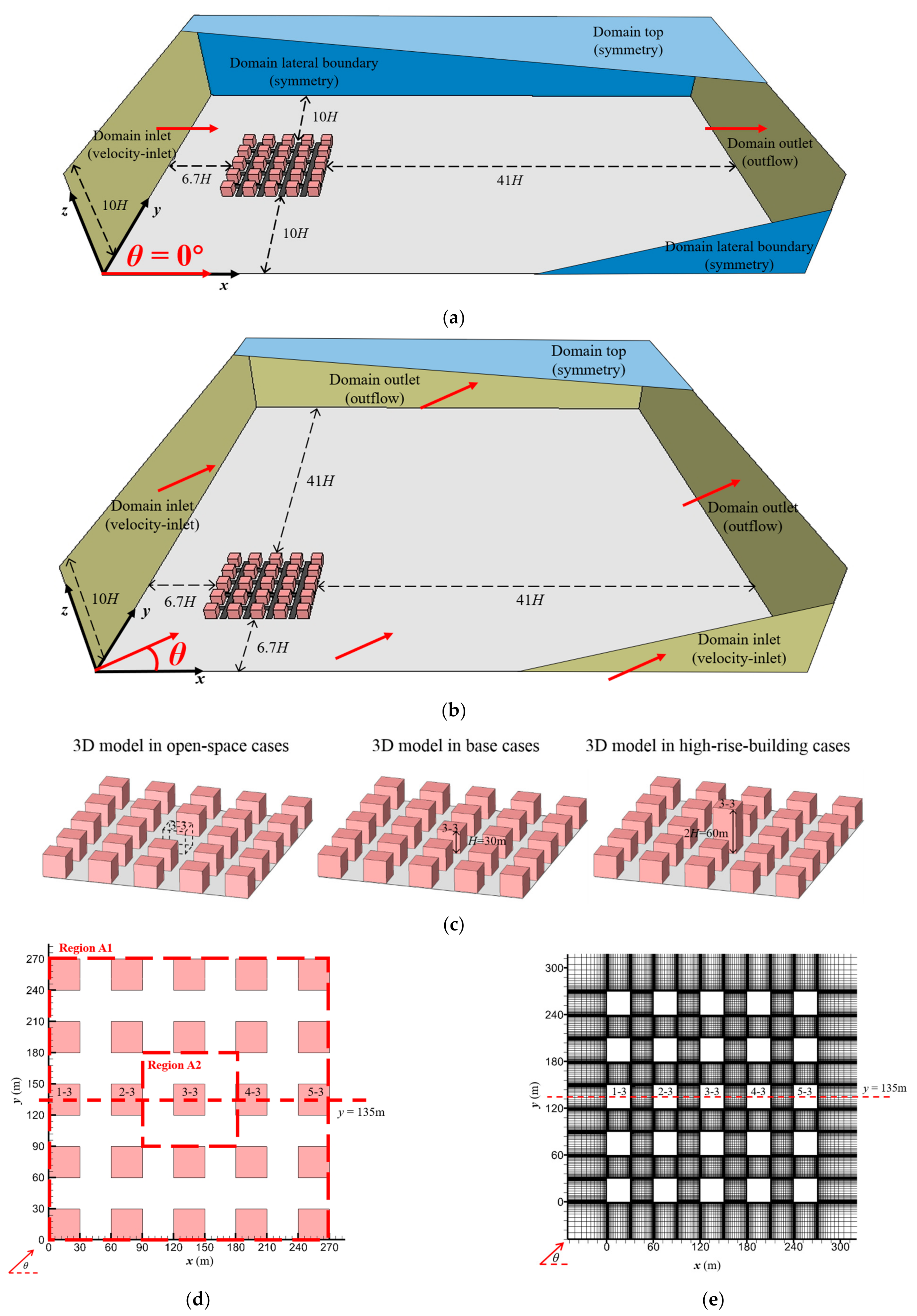


| Building Arrangement | Vegetation Planning | Wind Direction (θ) | Case Name |
|---|---|---|---|
| Base | Tree-free | 0°, 15°, 30°, 45° | [Base, θ] |
| With tree | 0°, 15°, 30°, 45° | [Base-tree, θ] | |
| Open space | Tree-free | 0°, 15°, 30°, 45° | [Open, θ] |
| With tree | 0°, 15°, 30°, 45° | [Open-tree, θ] | |
| High-rise building | Tree-free | 0°, 15°, 30°, 45° | [High, θ] |
| With tree | 0°, 15°, 30°, 45° | [High-tree, θ] |
Publisher’s Note: MDPI stays neutral with regard to jurisdictional claims in published maps and institutional affiliations. |
© 2022 by the authors. Licensee MDPI, Basel, Switzerland. This article is an open access article distributed under the terms and conditions of the Creative Commons Attribution (CC BY) license (https://creativecommons.org/licenses/by/4.0/).
Share and Cite
Li, Q.; Liang, J.; Wang, Q.; Chen, Y.; Yang, H.; Ling, H.; Luo, Z.; Hang, J. Numerical Investigations of Urban Pollutant Dispersion and Building Intake Fraction with Various 3D Building Configurations and Tree Plantings. Int. J. Environ. Res. Public Health 2022, 19, 3524. https://doi.org/10.3390/ijerph19063524
Li Q, Liang J, Wang Q, Chen Y, Yang H, Ling H, Luo Z, Hang J. Numerical Investigations of Urban Pollutant Dispersion and Building Intake Fraction with Various 3D Building Configurations and Tree Plantings. International Journal of Environmental Research and Public Health. 2022; 19(6):3524. https://doi.org/10.3390/ijerph19063524
Chicago/Turabian StyleLi, Qingman, Jie Liang, Qun Wang, Yuntong Chen, Hongyu Yang, Hong Ling, Zhiwen Luo, and Jian Hang. 2022. "Numerical Investigations of Urban Pollutant Dispersion and Building Intake Fraction with Various 3D Building Configurations and Tree Plantings" International Journal of Environmental Research and Public Health 19, no. 6: 3524. https://doi.org/10.3390/ijerph19063524
APA StyleLi, Q., Liang, J., Wang, Q., Chen, Y., Yang, H., Ling, H., Luo, Z., & Hang, J. (2022). Numerical Investigations of Urban Pollutant Dispersion and Building Intake Fraction with Various 3D Building Configurations and Tree Plantings. International Journal of Environmental Research and Public Health, 19(6), 3524. https://doi.org/10.3390/ijerph19063524