Drag Effect of Economic Growth and Its Spatial Differences under the Constraints of Resources and Environment: Empirical Findings from China’s Yellow River Basin


Abstract
:1. Introduction
2. Material and Methods
2.1. Variable Selection and Data Sources
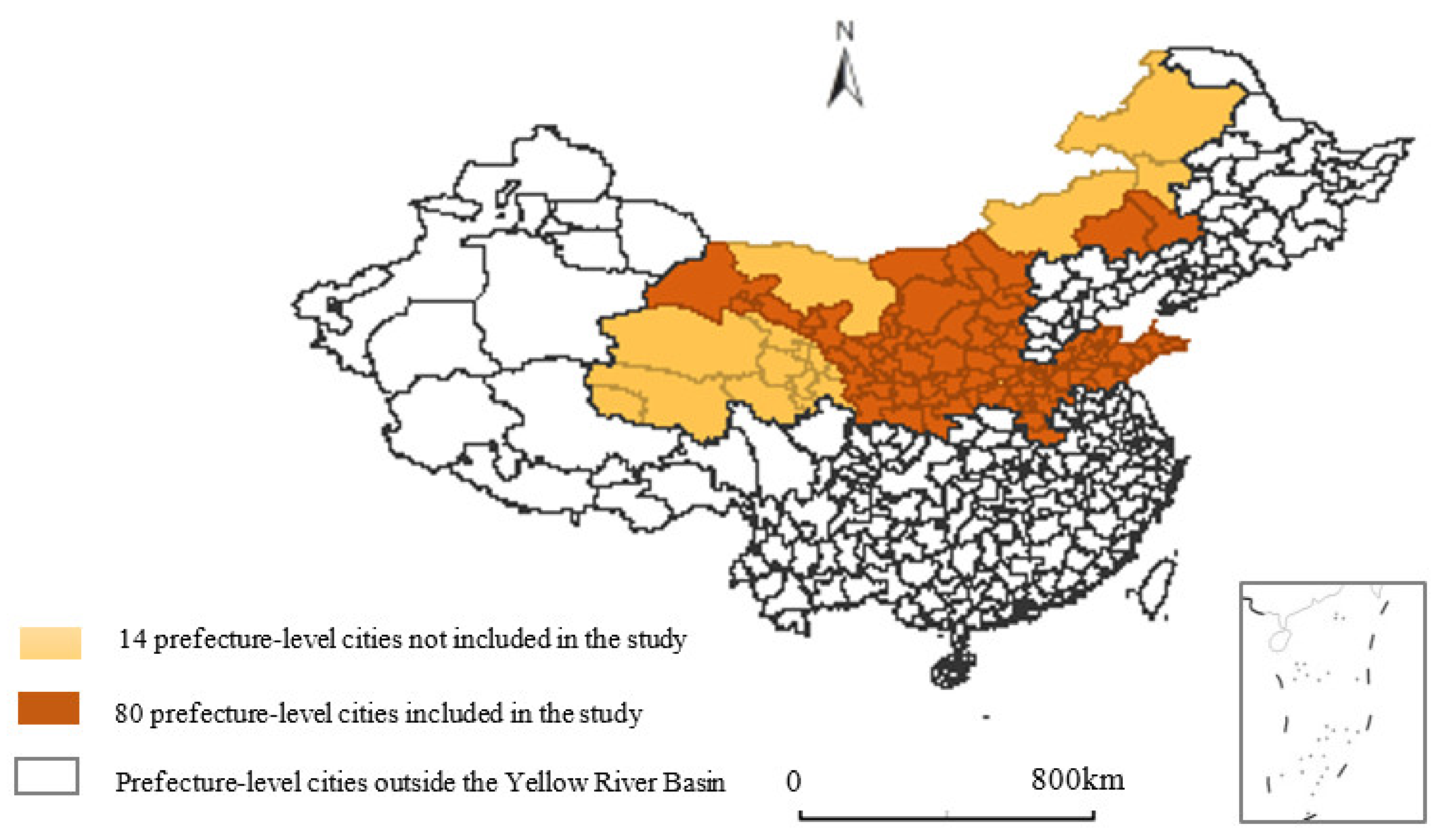
2.1.1. Research Object
2.1.2. Selection, Processing, and Data Sources of Specific Variables
2.1.3. Data Sources and Descriptive Statistical Analysis
2.2. Methods and Models
2.2.1. Construction of a Drag Effect Model of Economic Growth in the Yellow River Basin under Resource and Environmental Constraints
2.2.2. Construction of a Panel Model for the Economic Growth Drag Effect of the Yellow River Basin
- (1)
- Construction of classic panel model
- (2)
- Spatial Durbin model construction
3. Drag Effects Analysis and Discussion
3.1. Three Types of Drag Effects in a Single Prefecture-Level City
3.2. Regional Differences in Natural Resource Drag Effects
3.3. Regional Differences in Environmental Pollution Drag Effects
3.4. Regional Differences in Total Drag Effects
4. Spatial Effect Results and Discussion
4.1. Analysis of the Results of Classic Panel Regression and Spatial Regression of Drag Effects
4.2. Analysis of the Drag Effect Results under the Classic Panel Model and SDM
4.3. The Economic Growth Drag Effect Results of the Upper, Middle, and Lower Reaches of the Yellow River Basin
4.4. Further Discussion
5. Conclusions and Policy Recommendations
5.1. Main Conclusions
5.2. Policy Suggestion
Author Contributions
Funding
Institutional Review Board Statement
Informed Consent Statement
Data Availability Statement
Conflicts of Interest
Abbreviations
| CGE | Computable general equilibrium |
| SDM | Spatial Durbin model |
| GDP | Gross domestic product |
| SAR | Spatial autoregressive model |
| LLC | Levin, Lin, and Chu test |
| SEM | Spatial error model |
| IPS | Im, Pesaran, and Shin test |
| LR | Likelihood ratio test |
References
- Liu, Y.B.; Xiao, X.D.; Shao, C. Dynamic transformation mechanism and spatial heterogeneity analysis of water and soil resource constraints in the Yangtze River Economic Zone—Based on smooth panel transformation model and trend surface test. China Popul. Resour. Environ. 2019, 29, 89–98. [Google Scholar]
- Li, S.X.; Wang, N.; Wu, Q.S.; Cheng, J.H. The economic growth drag effect and its characteristics under energy and environmental constraints in poverty-stricken areas—An empirical study based on panel data of 21 provinces in China from 2000 to 2017. Quant. Econ. Res. 2020, 37, 42–60. [Google Scholar]
- Weitzman, M. Comments and Discussion (on “Lethal Model 2: The Limits to Growth Revisisted” by William D. Nordhaus). J. Brook. Pap. Econ. Act. 1992, 2, 50–54. [Google Scholar]
- Barbier, E.B. Endogenous Growth and Natural Resource Scarcity. J. Environ. Resour. Econ. 1999, 14, 51–74. [Google Scholar] [CrossRef]
- Bruvoll, A.; Glomsrod, S.; Vennemo, H. Environmental drag: Evidence from Norway. J. Ecol. Econ. 1999, 30, 235–249. [Google Scholar] [CrossRef]
- Romer, D. Advanced Macroeconomics, 2nd ed.; Shanghai University of Finance & Economics Press: Shanghai, China, 2001; pp. 30–38. [Google Scholar]
- Tsur, Y.; Zemel, A. Scarcity, growth and R&D. J. Environ. Econ. Manag. 2005, 49, 484–499. [Google Scholar]
- Brock, W.A.; Taylor, M.S. Economic Growth and the Environment: A Review of Theory and Empirics. Handb. Econ. Growth 2005, 1, 1749–1821. [Google Scholar]
- Copeland, B.R.; Taylor, M.S. Trade, Growth and the Environment. J. Econ. Lit. 2004, 42, 7–71. [Google Scholar] [CrossRef]
- Eriksson, C. Phasing out a polluting input in a growth model with directed technological change. Econ. Model. 2018, 68, 461–474. [Google Scholar] [CrossRef]
- Fatai, O.O. Tracking Unemployment Through Economic Growth, Export & FDI Inflows in Nigeria: An Application of Bound Test Approach. Soc. Sci. Med. 2016, 8, 218–229. [Google Scholar]
- Andersen, T.B.; Dalgaard, C.J. Power outages and economic growth in Africa. Energy Econ. 2013, 38, 19–23. [Google Scholar] [CrossRef] [Green Version]
- Sangmin, S.; Heekyung, P. Achieving cost-efficient diversification of water infrastructure system against uncertainty using modern portfolio theory. J. Hydroinformatics 2018, 20, 739–750. [Google Scholar]
- Boryczko, K.; Rak, J. Method for Assessment of Water Supply Diversification. Resources 2020, 9, 87. [Google Scholar] [CrossRef]
- Morton, H. Diversifying Water Sources with Potable Water Reuse. Water 2021, 2, 21. [Google Scholar]
- Xue, J.B.; Wang, Z.; Zhu, J.W.; Bing, W. Analysis of the “drag effect” of China’s economic growth. Financ. Res. 2004, 9, 5–14. [Google Scholar]
- Cui, Y. Analysis of the “drag effect” of Land Resources in China’s economic growth. Econ. Theory Econ. Manag. 2007, 11, 32–37. [Google Scholar]
- Wang, J.T. Study on the drag effect of land resources in China’s regional economic growth. Econ. Geogr. 2010, 30, 2067–2072, 2121. [Google Scholar]
- Luo, L.P. Study on the drag effect model of land resource growth based on virtual land growth. Seeker 2011, 2, 95–96. [Google Scholar]
- Xie, S.L.; Wang, Z.; Xue, J.B. Analysis of the “growth effect” of water and land resources in China’s economic development. Manag. World 2005, 7, 22–25+54. [Google Scholar]
- Liu, Y.B.; Yang, X.M.; Zhou, R.H.; Duan, Y.F.; Yao, C.S. Comparative study on the “growth effect” of water and land resources in the economic growth of the central region. Resour. Sci. 2011, 33, 1781–1787. [Google Scholar]
- Wan, Y.K.; Dong, S.C.; Wang, J.N.; Mao, Q.Y.; Liu, J.J. Research on the damping effect of Beijing water and soil resources on economic growth. Resour. Sci. 2012, 34, 475–480. [Google Scholar]
- Zhao, C.J.; Wu, B.J.; Wu, Y.M. Study on the effects of land resources on urban economic growth in the Yangtze River Delta metropolitan area. Ecol. Econ. 2018, 34, 81–85. [Google Scholar]
- Cao, C.; Chen, J.; Ding, C.C.; Xia, Y. Comparative study on the “drag effect” of the virtual cultivated land resources implied in the agricultural economic growth in the middle and lower reaches of the Yangtze River. China Agric. Resour. Reg. Plan. 2020, 41, 20–26. [Google Scholar]
- Sun, X.L.; Deng, F. An Empirical Analysis of the restrictive effect of water resources on economic growth in arid areas—taking Xinjiang as an example. Xinjiang Soc. Sci. 2013, 2, 43–47. [Google Scholar]
- Li, Y.; Shen, K.R. Energy structure constraints and China’s economic growth—Based on the measurement test of energy “End Effect”. J. Resour. Sci. 2010, 32, 2192–2199. [Google Scholar]
- Xu, D.L.; Li, Y. An Empirical study on the impact of energy constraints on economic growth and urbanization—Taking shandong province as an example. J. Beijing Inst. Technol. Soc. Sci. Ed. 2012, 14, 74–79, 88. [Google Scholar]
- Zhang, S.J. Analysis of the energy drag effect of regional economic growth—Taking wanjiang urban belt as an example. East China Econ. Manag. 2013, 27, 58–61. [Google Scholar]
- Shen, K.R.; Li, Y. Analysis of the energy drag effect of China’s economic growth. Ind. Econ. Res. 2010, 2, 1–8. [Google Scholar]
- Liu, Y.B.; Yang, X.M. Analysis of the “drag Effect” of resources and environment in the process of urbanization based on the theory of endogenous economic growth. China Popul. Resour. Environ. 2011, 21, 24–30. [Google Scholar]
- Li, F.; Zhang, J.; Zhang, F.L. The quantitative analysis of the “drag Effect” of resources and environment in the process of Xinjiang’s new industrialization. Stat. Decis. 2014, 13, 138–140. [Google Scholar]
- Gao, Y.; Feng, Z.X. Study on the “drag effect” of energy and environmental constraints in the process of urbanization. J. Xi’an Jiaotong Univ. Soc. Sci. Ed. 2018, 38, 44–50. [Google Scholar]
- Zhong, K.Y. Does the digital finance revolution validate the Environmental Kuznets Curve? Empirical findings from China. PLoS ONE 2022, 17, e0257498. [Google Scholar] [CrossRef]
- Sun, W. Analysis of the temporal and spatial differences of urban energy eco-efficiency in the Yellow River Basin and its influencing factors. J. Anhui Norm. Univ. Humanit. Soc. Sci. Ed. 2020, 48, 149–157. [Google Scholar]
- Zhang, J.; Wu, G.Y.; Zhang, J.P. Estimation of China’s inter-provincial material capital stock: 1952–2000. Econ. Res. J. 2004, 10, 35–44. [Google Scholar]
- Wang, X.L. The sustainability of China’s economic growth and institutional reform. Econ. Res. 2000, 7, 3–15. [Google Scholar]
- Zhong, K.Y.; Wang, Y.F.; Pei, J.M.; Tang, S.M.; Han, Z.L. Super Efficiency SBM-DEA and Neural Network for Performance Evaluation. Inf. Process. Manag. 2021, 58, 102728. [Google Scholar] [CrossRef]
- Zhong, K.; Li, C.; Wang, Q. Evaluation of Bank Innovation Efficiency with Data Envelopment Analysis: From the Perspective of Uncovering the Black Box between Input and Output. Mathematics 2021, 9, 3318. [Google Scholar] [CrossRef]
- Qin, T.; Zhang, H.Q.; Tong, J.P. Analysis of water resources constraint effect in the process of urbanization in the Yangtze River economic belt. China Popul. Resour. Environ. 2018, 28, 39–45. [Google Scholar]
- Zhang, L.; Duan, Q.L.; Wang, L.L. The Yellow River Basin Ecological Protection and High-Quality Development Report (2020); Social Science Literature Press: Beijing, China, 2020. [Google Scholar]

| Main Variable | Unit | Sample Size | Mean | Standard Deviation | Minimum | Maximum |
|---|---|---|---|---|---|---|
| GDP (Y) | Ten thousand yuan | 1280 | 10,996,580 | 12,720,747 | 210,687 | 92,433,263 |
| Capital stock (K) | Ten thousand yuan | 1280 | 10,840,525 | 12,443,174 | 207,025 | 82,804,866 |
| Effective labor (AL) | Hour | 1280 | 3,501,236 | 3,405,758 | 323,281 | 23,001,356 |
| Energy resources (E) | Ten thousand cubic meters | 1280 | 17,076 | 35,771 | 1 | 745,182 |
| Water resources (W) | Ten thousand cubic meters | 1280 | 184,266 | 245,450 | 205 | 2,279,600 |
| Land Resources (R) | Square kilometers | 1280 | 90 | 85 | 3 | 658 |
| Industrial wastewater discharge (B) | Ten thousand tons | 1280 | 5110 | 4799 | 99 | 28,191 |
| Industrial SO2 emissions (S) | Ton | 1280 | 65,786 | 55,031 | 633 | 337,164 |
| Industrial smoke (dust) emissions (D) | Ton | 1280 | 35,792 | 96,929 | 56 | 3,153,822 |
| Prefecture-Level City | Taiyuan | Datong | Yangquan | Changzhi | Jincheng | Shuozhou | Jinzhong | Yuncheng | Xinzhou | Linfen |
|---|---|---|---|---|---|---|---|---|---|---|
| Natural resource drag effect (%) | 0.4927 | 0.0716 | 0.0060 | −0.7223 | −0.4131 | −0.0095 | 0.2236 | 0.0931 | −0.6147 | −0.3503 |
| Environmental pollution drag effect (%) | 0.0252 | −0.7414 | −0.0088 | −0.3926 | −0.3090 | −0.5690 | 0.2258 | −0.0976 | 0.0731 | −0.0153 |
| Total drag effect (%) | 0.5179 | −0.6698 | −0.0029 | −1.1149 | −0.7221 | −0.5785 | 0.4495 | −0.0045 | −0.5417 | −0.3655 |
| Prefecture-level city | Luliang | Hohhot | Baotou | Wuhai | Chifeng | Tongliao | Ordos | Bayannaoer | Wulanchabu | Jinan |
| Natural resource drag effect (%) | −1.0134 | 0.1691 | 6.1147 | 2.2561 | −0.0813 | −0.0775 | 0.9787 | 0.6402 | 0.0553 | −0.7025 |
| Environmental pollution drag effect (%) | −0.0380 | −0.2319 | 1.7951 | −0.4369 | −0.4860 | −0.2778 | −0.0444 | −3.4039 | −0.4091 | 0.2631 |
| Total drag effect (%) | −1.0514 | −0.0628 | 7.9098 | 1.8192 | −0.5673 | −0.3553 | 0.9343 | −2.7637 | −0.3538 | −0.4394 |
| Prefecture-level city | Qingdao | Zibo | Zaozhuang | Dongying | Yantai | Weifang | Jining | Tai’an | Weihai | Rizhao |
| Natural resource drag effect (%) | −1.8576 | −0.0581 | 1.2073 | −0.8763 | 0.4128 | −0.3334 | −0.8016 | −0.6489 | 0.9906 | −1.4586 |
| Environmental pollution drag effect (%) | −1.8972 | −0.5157 | −0.2396 | 4.4830 | −0.1619 | −0.2317 | −0.5716 | −0.8008 | −0.3424 | −0.1671 |
| Total drag effect (%) | −3.7548 | −0.5738 | 0.9678 | 3.6067 | 0.2510 | −0.5651 | −1.3733 | −1.4497 | 0.6482 | −1.6257 |
| Prefecture-level city | Laiwu | Linyi | Dezhou | Liaocheng | Binzhou | Heze | Zhengzhou | Kaifeng | Luoyang | Pingdingshan |
| Natural resource end effect (%) | −0.2070 | −1.3444 | −0.8130 | −1.8578 | −0.5795 | −0.7496 | −0.2396 | −0.6379 | 0.8049 | −0.1847 |
| Environmental pollution drag effect (%) | −0.4381 | 0.1050 | −0.3704 | −0.0429 | −0.3331 | −0.1279 | −0.0860 | −0.0940 | −1.2916 | −0.3614 |
| Total drag effect (%) | −0.6451 | −1.2395 | −1.1833 | −1.9008 | −0.9126 | −0.8775 | −0.3256 | −0.7318 | −0.4867 | −0.5461 |
| Prefecture-level city | Anyang | Hebi | Xinxiang | Jiaozuo | Puyang | Xuchang | Luohe | Sanmenxia | Nanyang | Shangqiu |
| Natural resource drag effect (%) | −4.3472 | −1.1519 | −6.6325 | −0.0195 | −0.8639 | 3.9397 | −0.7620 | −1.1178 | −0.8147 | 0.1011 |
| Environmental pollution drag effect (%) | 1.0026 | 0.1850 | 10.1779 | −0.6514 | −0.5565 | −1.4055 | −0.5307 | −0.3594 | −0.4254 | −0.5957 |
| Total drag effect (%) | −3.3446 | −0.9669 | 3.5454 | −0.6708 | −1.4204 | 2.5342 | −1.2927 | −1.4771 | −1.2400 | −0.4946 |
| Prefecture-level city | Xinyang | Zhoukou | Zhumadian | Xi’an | Tongchuan | Baoji | Xianyang | Weinan | Yan’an | Hanzhong |
| Natural resource drag effect (%) | −1.0078 | −0.4242 | 0.1748 | 0.0980 | −0.9570 | 13.6347 | 0.3095 | −3.9266 | −0.8350 | 0.0514 |
| Environmental pollution drag effect (%) | 0.0345 | −0.1908 | −0.2540 | −0.2063 | −0.2357 | −61.5083 | −0.6221 | 0.0346 | −0.0935 | −0.1571 |
| Total drag effect (%) | −0.9733 | −0.6150 | −0.0791 | −0.1082 | −1.1927 | −47.8737 | −0.3126 | −3.8921 | −0.9285 | −0.1057 |
| Prefecture-level city | Yulin | Ankang | Shangluo | Lanzhou | Jiayuguan | Jinchang | Silver | Tianshui | Wuwei | Zhangye |
| Natural resource drag effect (%) | −1.6976 | −0.1051 | −1.3425 | −0.1793 | 0.0190 | 0.2086 | −0.7379 | 0.0748 | −0.4381 | 0.0154 |
| Environmental pollution drag effect (%) | −0.5067 | −0.6294 | −0.1335 | −0.4824 | −0.4174 | 0.1237 | 0.2605 | 0.1535 | −0.0879 | −0.1803 |
| Total drag effect (%) | −2.2043 | −0.7344 | −1.4761 | −0.6617 | −0.3985 | 0.3323 | −0.4775 | 0.2283 | −0.5260 | −0.1649 |
| Prefecture-level city | Pingliang | Jiuquan | Qingyang | Dingxi | Longnan | Yinchuan | Shizuishan | Wu Zhong | Guyuan | Zhongwei |
| Natural resource drag effect (%) | −1.4086 | 0.1662 | −0.1365 | −0.3527 | −0.3279 | −0.5504 | −0.1209 | −8.2142 | −0.2728 | 1.9752 |
| Environmental pollution drag effect (%) | −0.3701 | 0.1197 | 0.5258 | −0.8327 | −0.1287 | 0.0366 | −0.0427 | 0.6612 | 0.4016 | −0.8247 |
| Total drag effect (%) | −1.7786 | 0.2859 | 0.3893 | −1.1855 | −0.4566 | −0.5137 | −0.1635 | −7.5530 | 0.1288 | 1.1505 |
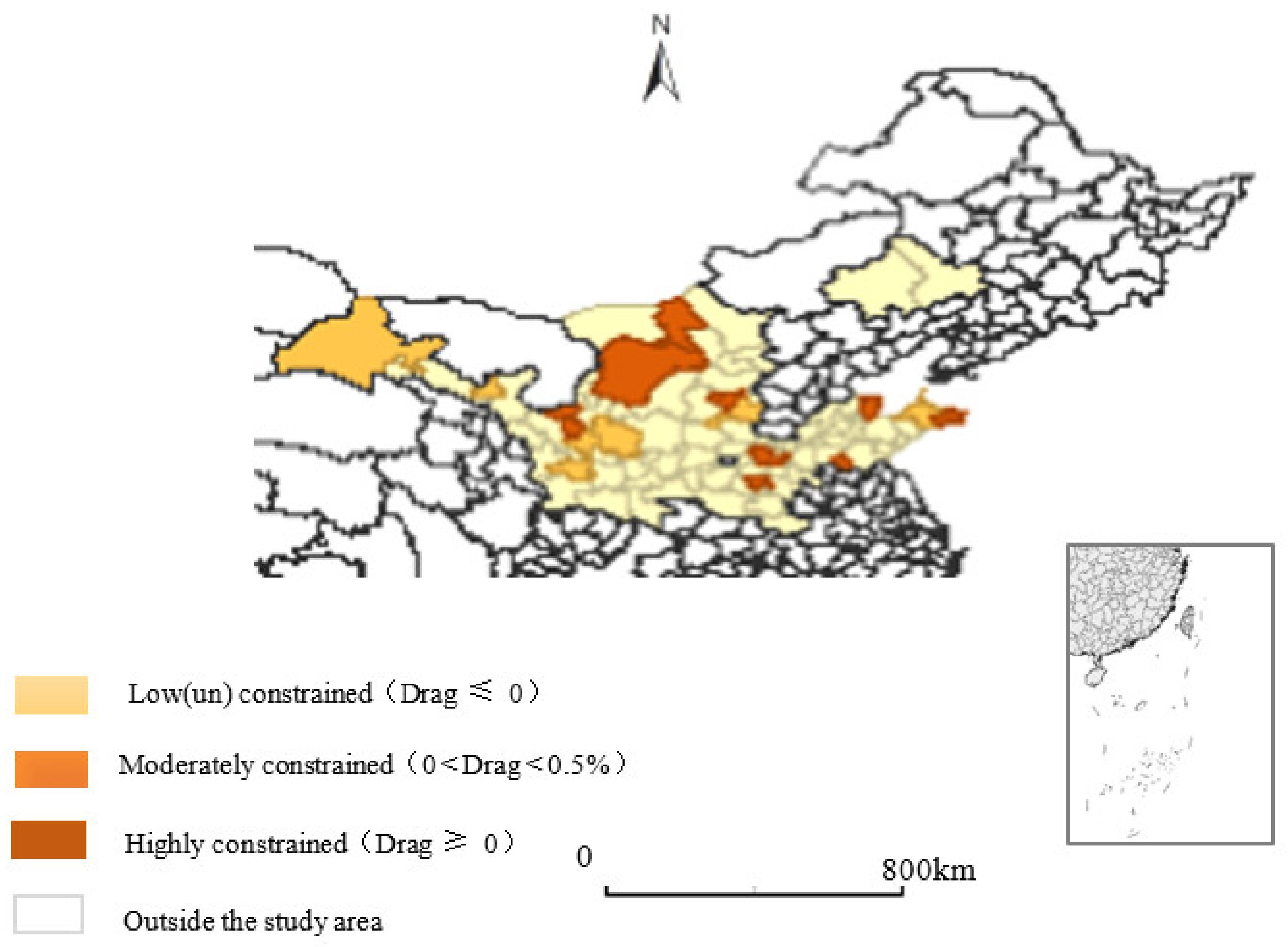
| Drag Effect Mode | Segmented Basins | Natural Resource Drag Effect | Environmental Pollution Drag Effect | Total Drag Effect |
|---|---|---|---|---|
| Low (un) constrained (Drag ≤ 0) | Upper Yellow River | Lanzhou, Baiyin, Wuwei, Pingliang, Qingyang, Dingxi, Longnan, Yinchuan, Shizuishan, Wuzhong, Guyuan (11) | Lanzhou, Jiayuguan, Wuwei, Zhangye, Pingliang, Dingxi, Longnan, Shizuishan, Zhongwei (9) | Lanzhou, Jiayuguan, Baiyin, Wuwei, Zhangye, Pingliang, Dingxi, Longnan, Yinchuan, Shizuishan, Wuzhong City (11) |
| Middle Yellow River | Changzhi, Jincheng, Shuozhou, Xinzhou, Linfen, Luliang, Tongchuan, Weinan, Yan’an, Yulin, Ankang, Shangluo, Chifeng, Tongliao (14) | Datong, Yangquan, Changzhi, Jincheng, Shuozhou, Yuncheng, Linfen, Luliang, Hohhot, Wuhai, Chifeng, Tongliao, Ordos, Bayanzhuoer, Ulanchabu, Xi’an, Tongchuan, Baoji, Xianyang, Yan’an, Hanzhong, Yulin, Ankang, Shangluo (24) | Datong, Yangquan, Changzhi, Jincheng, Shuozhou, Yuncheng, Xinzhou, Linfen, Luliang, Hohhot, Chifeng, Tongliao, Bayanzhuoer, Ulanchabu, Xi’an, Tongchuan, Baoji, Xianyang, Weinan, Yan’an, Hanzhong, Yulin, Ankang, Shangluo (24) | |
| Lower Yellow River | Jinan, Qingdao, Zibo, Dongying, Weifang, Jining, Taian, Rizhao, Laiwu, Linyi, Dezhou, Liaocheng, Binzhou, Heze, Zhengzhou, Kaifeng, Pingdingshan, Anyang, Hebi, Xinxiang, Jiaozuo, Puyang, Luohe, Sanmenxia, Nanyang, Xinyang, Zhoukou (27) | Qingdao, Zibo, Zaozhuang, Yantai, Weifang, Jining, Taian, Weihai, Rizhao, Laiwu, Dezhou, Liaocheng, Binzhou, Heze, Zhengzhou, Kaifeng, Luoyang, Pingdingshan, Jiaozuo, Puyang, Xuchang, Luohe, Sanmenxia, Nanyang, Shangqiu, Zhoukou, Zhumadian (27) | Jinan, Qingdao, Zibo, Weifang, Jining, Taian, Rizhao, Laiwu, Linyi, Dezhou, Liaocheng, Binzhou, Heze, Zhengzhou, Kaifeng, Luoyang, Pingdingshan, Anyang, Hebi, Jiaozuo, Puyang, Luohe, Sanmenxia, Nanyang, Xinyang, Shangqiu, Zhoukou, Zhumadian (28) | |
| Moderately constrained (0 < Drag < 0.5%) | Upper Yellow River | Jiayuguan, Jinchang, Tianshui, Zhangye, Jiuquan (5) | Jinchang, Baiyin, Tianshui, Jiuquan, Yinchuan, Guyuan (6) | Jinchang, Tianshui, Jiuquan, Qingyang, Guyuan (5) |
| Middle Yellow River | Hohhot, Ulan Chabu, Xi’an, Xianyang, Hanzhong, Taiyuan, Datong, Yangquan, Jinzhong, Yuncheng (10) | Taiyuan, Jinzhong, Xinzhou, Weinan (4) | Jinzhong (1) | |
| Lower Yellow River | Yantai, Shangqiu, Zhuma (3) | Jinan, Linyi, Hebi, Xinyang (4) | Yantai (1) | |
| Highly constrained (Drag ≥ 0.5%) | Upper Yellow River | Zhongwei (1) | Qingyang, Wu Zhong (2) | Zhongwei (1) |
| Middle Yellow River | Baotou, Wuhai, Ordos, Bayannaoer, Baoji (5) | Baotou (1) | Taiyuan, Baotou, Wuhai, Ordos (4) | |
| Lower Yellow River | Zaozhuang, Weihai, Luoyang, Xuchang (4) | Dongying, Anyang, Xinxiang (3) | Zaozhuang, Dongying, Weihai, Xinxiang, Xuchang (5) |
| Variable | Classic Panel Model | SDM | Direct Effect | Indirect Effect | Total Effect | Weight Variable | SDM |
|---|---|---|---|---|---|---|---|
| lnK | 0.767 *** | 0.6873 *** | 0.6480 *** | −0.4456 * | 0.2024 | WlnK | −6.4610 *** |
| (29.25) | (6.6800) | (6.6400) | (−1.8500) | (0.8500) | (−5.3800) | ||
| lnAL | 0.0415 | 0.0316 ** | 0.0016 | −0.3040 *** | −0.3030 ** | WlnAL | −0.0992 *** |
| (1.59) | (2.0450) | (0.0780) | (−2.9890) | (−2.6560) | (−3.7670) | ||
| lnE | 0.0168 *** | −0.0041 * | −0.0060 * | −0.0224 | −0.0284 | WlnE | −0.0022 |
| (4.11) | (−1.75) | (−1.92) | (−1.32) | (−1.47) | (−0.5160) | ||
| lnW | 0.148 *** | 0.0240 ** | 0.0471 *** | 0.2410 *** | 0.2880 ** | WlnW | 0.0395 ** |
| (7.62) | (2.2450) | (3.1180) | (2.7370) | (2.8780) | (2.0250) | ||
| lnR | 0.170 *** | 0.0752 *** | 0.1200 *** | 0.4580 *** | 0.5770 *** | WlnR | 0.0543 * |
| (5.82) | (4.7780) | (5.0270) | (3.1780) | (3.5350) | (1.7450) | ||
| lnB | −0.110 *** | −0.0412 *** | −0.0860 *** | −0.4670 *** | −0.5530 *** | WlnB | −0.0833 *** |
| (−7.05) | (−4.7450) | (−7.1000) | (−6.3189) | (−6.6670) | (−5.1170) | ||
| lnS | −0.0542 *** | 0.0443 *** | 0.0667 *** | 0.2330 *** | 0.3000 *** | WlnS | 0.0235 * |
| (−4.80) | (5.9260) | (5.7270) | (3.7190) | (4.1450) | (1.7560) | ||
| lnD | 0.0712 *** | 0.0057 | 0.0102 | 0.0487 | 0.0589 | WlnD | 0.0070 |
| (6.79) | (0.9290) | (1.2560) | (0.9670) | (1.0350) | (0.6001) |
| Variable | Classic Panel Model | SDM | Direct Effect | Indirect Effect | Total Effect |
|---|---|---|---|---|---|
| Capital stock elasticity coefficient (α) | 0.767 | 0.6873 | 0.648 | −0.4456 | 0.2024 |
| Energy resource elasticity coefficient (β) | 0.0168 | −0.0041 | −0.006 | −0.0224 | −0.0284 |
| Water resource coefficient (φ) | 0.148 | 0.024 | 0.0471 | 0.241 | 0.288 |
| Elasticity coefficient of land resources (ν) | 0.17 | 0.0752 | 0.12 | 0.458 | 0.577 |
| Industrial wastewater discharge elasticity coefficient (δ) | −0.11 | −0.0412 | −0.086 | −0.467 | −0.553 |
| Industrial SO2 emission elasticity coefficient (ω) | −0.0542 | 0.0443 | 0.0667 | 0.233 | 0.3 |
| Industrial smoke emission elasticity coefficient (ψ) | 0.0712 | 0.0057 | 0.0102 | 0.0487 | 0.0589 |
| Natural resource end effect (%) | −0.7204 | 0.0095 | 0.0166 | −0.0659 | 0.439 |
| Environmental pollution drag effect (%) | −0.1143 | 0.0042 | 0.0082 | −0.0387 | 0.2501 |
| Total drag effect (%) | −0.8347 | 0.0137 | 0.0248 | −0.1045 | 0.6891 |
| Area | Upper Yellow River | Middle Yellow River | Lower Yellow River | |||||||||
|---|---|---|---|---|---|---|---|---|---|---|---|---|
| Variable | SDM | Direct Effect | Indirect Effect | Total Effect | SDM | Direct Effect | Indirect Effect | Total Effect | SDM | Direct Effect | Indirect Effect | Total Effect |
| lnK | 0.6826 *** | 0.6496 *** | −0.3036 *** | 0.3460 *** | 0.8360 *** | 0.8130 *** | −0.2210 ** | 0.5920 *** | −0.7548 *** | −0.7307 *** | 0.3403 *** | −0.3904 *** |
| (9.3300) | (9.5500) | (−2.6600) | (3.3500) | (13.5900) | (13.0900) | (−2.4200) | (5.3700) | (−7.5700) | (−7.5000) | (2.8700) | (−4.3300) | |
| lnAL | −0.1540 * | −0.3160 *** | −1.3470 *** | −1.6630 *** | −0.0088 | −0.0108 | 0.0016 | −0.0092 | −0.0108 * | −0.0116 ** | −0.0095 | −0.0211 |
| (−1.9500) | (−3.2400) | (−4.1400) | (−4.1600) | (−0.2200) | (−0.2500) | −0.0200 | (−0.0700) | (−1.9300) | (−2.1400) | (−0.6800) | (−1.3700) | |
| lnE | −0.0139 * | −0.0204 ** | −0.0621 *** | −0.0825 *** | 0.0080 * | 0.0157 *** | 0.0642 *** | 0.0799 *** | −0.0007 | −0.0017 | −0.0182 *** | −0.0199 *** |
| (−1.7800) | (−2.3600) | (−2.5600) | (−2.7700) | −1.9500 | −3.4400 | −3.5700 | −3.8700 | (−0.6900) | (−1.5900) | (−4.9000) | (−4.6100) | |
| lnW | 0.0087 | 0.0161 | 0.0695 | 0.0856 | 0.0435** | 0.0447** | 0.0117 | 0.0564 | 0.0241 *** | 0.0243 *** | 0.0050 | 0.0294 |
| (0.2500) | (0.4100) | (0.5900) | (0.6000) | (2.3700) | (2.0200) | (0.2000) | (0.7400) | (4.9100) | (4.9700) | (0.3800) | (1.9200) | |
| lnR | 0.1280 *** | 0.1770 *** | 0.4140 ** | 0.5910 ** | 0.06810 ** | 0.08290 ** | 0.1180 | 0.2010 * | 0.0115 * | 0.0129 * | 0.0218 | 0.0347 |
| (2.6100) | (2.9600) | (2.1900) | (2.5300) | (2.3500) | (2.4400) | (1.3700) | (1.7800) | (1.6600) | (1.7800) | (1.0900) | (1.4200) | |
| lnB | −0.0518 * | −0.0687 ** | −0.1570 * | −0.2250 ** | 0.0224 | 0.0323 | 0.0875 | 0.1200 | 0.0158 *** | 0.0133 *** | −0.0424 *** | −0.0291 ** |
| (−1.7900) | (−2.0900) | (−1.9400) | (−2.2000) | −1.3100 | −1.4800 | −1.0700 | −1.2200 | −4.0000 | −3.3000 | (−3.7600) | (−2.2200) | |
| lnS | 0.0417 * | 0.0291 | −0.1070 | −0.0783 | −0.0363 *** | −0.0550 *** | −0.160 *** | −0.215 *** | 0.0014 | 0.0022 | 0.0127 | 0.0148 |
| (1.8400) | (0.9400) | (−1.3600) | (−0.7400) | (−3.5200) | (−4.1600) | (−3.2300) | (−3.6700) | (0.3800) | (0.5200) | (1.2300) | (1.2100) | |
| lnD | −0.0147 | −0.0044 | 0.0906 | 0.0862 | 0.0211 | 0.0300 ** | 0.0752 *** | 0.1050 *** | −0.0105 *** | −0.0110 *** | −0.0063 | −0.0172 ** |
| (−0.7500) | (−0.2100) | (1.4300) | (1.1200) | (1.5700) | (2.2900) | (2.8800) | (3.3800) | (−4.0600) | (−4.5300) | (−0.8400) | (−2.0800) | |
| WlnK | −50.4400 *** | — | — | — | −0.6270 *** | — | — | — | 4.7140 *** | — | — | — |
| (−5.2200) | — | — | — | (−10.7500) | — | — | — | −4.0800 | — | — | — | |
| WlnAL | −0.7220 *** | — | — | — | 0.0103 | — | — | — | −0.0046 | — | — | — |
| (−4.1000) | — | — | — | −0.2500 | — | — | — | (−0.4300) | — | — | — | |
| WlnE | −0.0304 ** | — | — | — | 0.0200 ** | — | — | — | −0.0134 *** | — | — | — |
| (−2.0400) | — | — | — | −2.3800 | — | — | — | (−4.9600) | — | — | — | |
| WlnW | 0.0337 | — | — | — | −0.0207 | — | — | — | −0.0035 | — | — | — |
| −0.5200 | — | — | — | (−0.9900) | — | — | — | (−0.3700) | — | — | — | |
| WlnR | 0.1880 * | — | — | — | 0.0006 | — | — | — | 0.0133 | — | — | — |
| −1.8400 | — | — | — | −0.0200 | — | — | — | −0.9100 | — | — | — | |
| WlnB | −0.0712 | — | — | — | 0.0204 | — | — | — | −0.0371 *** | — | — | — |
| (−1.5800) | — | — | — | −0.7100 | — | — | — | (−4.5100) | — | — | — | |
| WlnS | −0.0814 ** | — | — | — | −0.0394 ** | — | — | — | 0.0098 | — | — | — |
| (−2.0200) | — | — | — | (−2.1000) | — | — | — | −1.2900 | — | — | — | |
| WlnD | 0.0596 | — | — | — | 0.0149 | — | — | — | −0.0021 | — | — | — |
| −1.6300 | — | — | — | −1.1000 | — | — | — | (−0.3900) | — | — | — | |
| Area | Upper Yellow River | Middle Yellow River | Lower Yellow River | |||||||||
|---|---|---|---|---|---|---|---|---|---|---|---|---|
| Variable | SDM | Direct Effect | Indirect Effect | Total Effect | SDM | Direct Effect | Indirect Effect | Total Effect | SDM | Direct Effect | Indirect Effect | Total Effect |
| Capital stock elasticity coefficient (α) | 0.6826 | 0.6496 | −0.3036 | 0.3460 | 0.8360 | 0.8130 | −0.2210 | 0.5920 | −0.7548 | −0.7307 | 0.3403 | −0.3904 |
| Energy resource elasticity coefficient (β) | −0.0139 | −0.0204 | −0.0621 | −0.0825 | 0.0080 | 0.0157 | 0.0642 | 0.0799 | −0.0007 | −0.0017 | −0.0182 | −0.0199 |
| Water resource coefficient (φ) | 0.0087 | 0.0161 | 0.0695 | 0.0856 | 0.0435 | 0.0447 | 0.0117 | 0.0564 | 0.0241 | 0.0243 | 0.0050 | 0.0294 |
| Elasticity coefficient of land resources (ν) | 0.1280 | 0.1770 | 0.4140 | 0.5910 | 0.0681 | 0.0829 | 0.1180 | 0.2010 | 0.0115 | 0.0129 | 0.0218 | 0.0347 |
| Industrial wastewater discharge elasticity coefficient (δ) | −0.0518 | −0.0687 | −0.1570 | −0.2250 | 0.0224 | 0.0323 | 0.0875 | 0.1200 | 0.0158 | 0.0133 | −0.0424 | −0.0291 |
| Industrial SO2 emission elasticity coefficient (ω) | 0.0417 | 0.0291 | −0.1070 | −0.0783 | −0.0363 | −0.0550 | −0.1600 | −0.2150 | 0.0014 | 0.0022 | 0.0127 | 0.0148 |
| Industrial smoke emission elasticity coefficient (ψ) | −0.0147 | −0.0044 | 0.0906 | 0.0862 | 0.0211 | 0.0300 | 0.0752 | 0.1050 | −0.0105 | −0.0110 | −0.0063 | −0.0172 |
| Average annual growth rate of labor (n) | 0.0079 | 0.0079 | 0.0079 | 0.0079 | 0.0070 | 0.0070 | 0.0070 | 0.0070 | 0.0047 | 0.0047 | 0.0047 | 0.0047 |
| Natural resource drag effect (%) | 0.0009 | 0.0013 | −0.0060 | 0.0081 | 0.3216 | −0.3527 | −0.0876 | −0.4241 | −0.0018 | 0.0019 | −0.0019 | −0.0023 |
| Environmental pollution drag effect (%) | 0.0005 | 0.0008 | −0.0063 | 0.0074 | 0.1100 | 0.1415 | 0.0603 | 0.2455 | −0.0014 | −0.0016 | 0.0124 | −0.0088 |
| Total drag effect (%) | 0.0014 | 0.0021 | −0.0123 | 0.0156 | 0.2116 | −0.2111 | −0.0274 | −0.1786 | −0.0032 | −0.0035 | 0.0105 | −0.0111 |
Publisher’s Note: MDPI stays neutral with regard to jurisdictional claims in published maps and institutional affiliations. |
© 2022 by the authors. Licensee MDPI, Basel, Switzerland. This article is an open access article distributed under the terms and conditions of the Creative Commons Attribution (CC BY) license (https://creativecommons.org/licenses/by/4.0/).
Share and Cite
Zhou, Y.; Li, D.; Li, W.; Mei, D.; Zhong, J. Drag Effect of Economic Growth and Its Spatial Differences under the Constraints of Resources and Environment: Empirical Findings from China’s Yellow River Basin. Int. J. Environ. Res. Public Health 2022, 19, 3027. https://doi.org/10.3390/ijerph19053027
Zhou Y, Li D, Li W, Mei D, Zhong J. Drag Effect of Economic Growth and Its Spatial Differences under the Constraints of Resources and Environment: Empirical Findings from China’s Yellow River Basin. International Journal of Environmental Research and Public Health. 2022; 19(5):3027. https://doi.org/10.3390/ijerph19053027
Chicago/Turabian StyleZhou, Yujiao, Ding Li, Weifeng Li, Dong Mei, and Jianyi Zhong. 2022. "Drag Effect of Economic Growth and Its Spatial Differences under the Constraints of Resources and Environment: Empirical Findings from China’s Yellow River Basin" International Journal of Environmental Research and Public Health 19, no. 5: 3027. https://doi.org/10.3390/ijerph19053027
APA StyleZhou, Y., Li, D., Li, W., Mei, D., & Zhong, J. (2022). Drag Effect of Economic Growth and Its Spatial Differences under the Constraints of Resources and Environment: Empirical Findings from China’s Yellow River Basin. International Journal of Environmental Research and Public Health, 19(5), 3027. https://doi.org/10.3390/ijerph19053027