
Seasonal and Diurnal Variation of Land Surface Temperature Distribution and Its Relation to Land Use/Land Cover Patterns


Abstract
1. Introduction
2. Data and Methods
2.1. Study Area
2.2. Data Sets
- For thermal data, we rely on multi-temporal data from the Landsat 8 Thermal Infrared Sensor (TIRS) and Operational Land Imager (OLI) data, which are publicly available (level-1-products http://earthexplorer.usgs.gov/ accessed 20 May 2020). The spatial resolution of Landsat 8 image bands is 30 m except for band 8 (panchromatic, 15 m spatial resolution) and the two thermal bands 10–11 (100 m). Conditions for images to be selected for the study, are: (1) cloud-free; (2) coverage of the entire study area; (3) four-season division covering spring (March–May), summer (June–August), autumn (September–November), and winter (December–February); and (4) daytime (local overpass time before noon) and nighttime (local overpass time after 8 p.m.). Based on these criteria, the following eight images between 2018 and 2019 were selected to retrieve LSTs in spring, summer, autumn, and winter as well as day and nighttime of Berlin (Table 1). The time of data acquisition was approximately 12:00 a.m. and 10:30 p.m. Greenwich Mean Time (GMT) in Berlin.
- The land use/land cover (LU/LC) data (10 m) of Berlin (Figure 2) in 2018 were obtained from the European Urban Atlas (https://land.copernicus.eu/local/urban-atlas accessed 18 February 2020), which provides reliable, inter-comparable, high-resolution data. The LU/LC classification includes six primary types (croplands, woodlands, grasslands, water areas, built-up lands, and unused lands) and 25 secondary types. We identified seven important classes (Table 2): Transportation (15.2%), Commercial and Industrial (6.7%), Residential (35.2%), Sports and Leisure (4.3%), Vegetation (30.2%), Agriculture (2.9%), Wetlands (5.5%) (the percentage of the corresponding class within the study area in 2018).
- Urban morphologic indicators were obtained from building footprints from Open Street Map (https://www.openstreetmap.org/ accessed on 1 January 2020).
2.3. Research Framework

2.4. Retrieving Land Surface Temperature
2.5. Selected LUCP Indicators
2.6. Statistical Analyses Relating Spatial Indicators and LST
3. Results
3.1. Spatial Distribution of LST
- (1)
- Very Hot Spot: LST ≥ LSTmean + 2Std;
- (2)
- Hot Spot: LSTmean + Std ≤ LST ≤ LSTmean + 2Std;
- (3)
- Warm spot: LSTmean ≤ LST ≤ LSTmean + Std;
- (4)
- Cool Spot: LSTmean − Std ≤ LST ≤ LSTmean;
- (5)
- Cold Spot: LSTmean − 2 Std ≤ LST ≤ LSTmean − Std;
- (6)
- Very Cold Spot: LST ≤ LSTmean − 2Std.
3.2. Land Cover Analysis of LST
3.3. Spatial-Temporal Patterns of LUCP Indicators
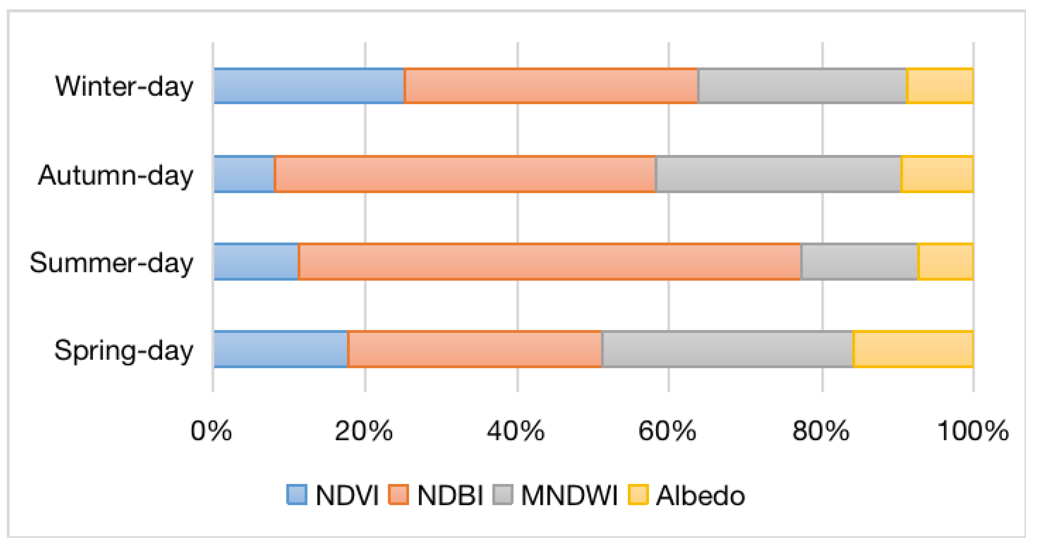
3.4. Correlation between LST and LUCP Indicators
- In spring, NDBI (0.335) > MNDWI (0.330) > NDVI (0.177) > Albedo (0.158);
- In summer, NDBI (0.660) > MNDWI (0.155) > NDVI (0.112) > Albedo (0.073);
- In autumn, NDBI (0.502) > MNDWI (0.321) > NDVI (0.082) > Albedo (0.095);
- In winter, NDBI (0.388) > MNDWI (0.274) > NDVI (0.251) > Albedo (0.087).
- In summer, BD (0.334) > ISF (0.235) > FAR (0.220) > BH (0.211);
- In autumn, ISF (0.384) > BH (0.249) > FAR (0.227) > BD (0.139);
- In winter, FAR (0.333) > ISF (0.271) > BD (0.212) > BH (0.183).

4. Discussion
4.1. Investigation of Seasonal Variations in Urban Thermal Environment
4.2. Implications for Urban Planning and Management
4.3. Limitations and Future Studies
5. Conclusions
Author Contributions
Funding
Institutional Review Board Statement
Informed Consent Statement
Data Availability Statement
Acknowledgments
Conflicts of Interest
References
- Voogt, J.A.; Oke, T.R. Thermal Remote Sensing of Urban Climates. Remote Sens. Environ. 2003, 86, 370–384. [Google Scholar] [CrossRef]
- Stone, B.; Rodgers, M.O. Urban Form and Thermal Efficiency: How the Design of Cities Influences the Urban Heat Island Effect. J. Am. Plan. Assoc. 2001, 67, 186–198. [Google Scholar] [CrossRef]
- Simwanda, M.; Ranagalage, M.; Estoque, R.C.; Murayama, Y. Spatial Analysis of Surface Urban Heat Islands in Four Rapidly Growing African Cities. Remote Sens. 2019, 11, 1645. [Google Scholar] [CrossRef]
- Sarrat, C.; Lemonsu, A.; Masson, V.; Guedalia, D. Impact of Urban Heat Island on Regional Atmospheric Pollution. Atmos. Environ. 2006, 40, 1743–1758. [Google Scholar] [CrossRef]
- Harlan, S.L.; Brazel, A.J.; Prashad, L.; Stefanov, W.L.; Larsen, L. Neighborhood Microclimates and Vulnerability to Heat Stress. Soc. Sci. Med. 2006, 63, 2847–2863. [Google Scholar] [CrossRef]
- Schwarz, N.; Schlink, U.; Franck, U.; Großmann, K. Relationship of Land Surface and Air Temperatures and Its Implications for Quantifying Urban Heat Island Indicators—An Application for the City of Leipzig (Germany). Ecol. Indic. 2012, 18, 693–704. [Google Scholar] [CrossRef]
- Rizwan, A.M.; DENNIS, L.Y.C.; LIU, C. A Review on the Generation, Determination and Mitigation of Urban Heat Island. J. Environ. Sci. 2008, 20, 120–128. [Google Scholar] [CrossRef]
- Weng, Q.; Lu, D.; Schubring, J. Estimation of Land Surface Temperature–Vegetation Abundance Relationship for Urban Heat Island Studies. Remote Sens. Environ. 2004, 89, 467–483. [Google Scholar] [CrossRef]
- Weng, Q. Thermal Infrared Remote Sensing for Urban Climate and Environmental Studies: Methods, Applications, and Trends. ISPRS J. Photogramm. Remote Sens. 2009, 64, 335–344. [Google Scholar] [CrossRef]
- Imhoff, M.L.; Zhang, P.; Wolfe, R.E.; Bounoua, L. Remote Sensing of the Urban Heat Island Effect across Biomes in the Continental USA. Remote Sens. Environ. 2010, 114, 504–513. [Google Scholar] [CrossRef]
- Myint, S.W.; Wentz, E.A.; Brazel, A.J.; Quattrochi, D.A. The Impact of Distinct Anthropogenic and Vegetation Features on Urban Warming. Landsc. Ecol. 2013, 28, 959–978. [Google Scholar] [CrossRef]
- Arnfield, A.J. Two Decades of Urban Climate Research: A Review of Turbulence, Exchanges of Energy and Water, and the Urban Heat Island. Int. J. Climatol. 2003, 23, 1–26. [Google Scholar] [CrossRef]
- Peng, J.; Xie, P.; Liu, Y.; Ma, J. Urban Thermal Environment Dynamics and Associated Landscape Pattern Factors: A Case Study in the Beijing Metropolitan Region. Remote Sens. Environ. 2016, 173, 145–155. [Google Scholar] [CrossRef]
- Wang, J.; Qingming, Z.; Guo, H.; Jin, Z. Characterizing the Spatial Dynamics of Land Surface Temperature–Impervious Surface Fraction Relationship. Int. J. Appl. Earth Obs. Geoinf. 2016, 45, 55–65. [Google Scholar] [CrossRef]
- Scarano, M.; Mancini, F. Assessing the Relationship between Sky View Factor and Land Surface Temperature to the Spatial Resolution. Int. J. Remote Sens. 2017, 38, 6910–6929. [Google Scholar] [CrossRef]
- Sun, F.; Liu, M.; Wang, Y.; Wang, H.; Che, Y. The Effects of 3D Architectural Patterns on the Urban Surface Temperature at a Neighborhood Scale: Relative Contributions and Marginal Effects. J. Clean. Prod. 2020, 258, 120706. [Google Scholar] [CrossRef]
- Yuan, F.; Bauer, M.E. Comparison of Impervious Surface Area and Normalized Difference Vegetation Index as Indicators of Surface Urban Heat Island Effects in Landsat Imagery. Remote Sens. Environ. 2007, 106, 375–386. [Google Scholar] [CrossRef]
- Oke, T.R. The Energetic Basis of the Urban Heat Island. Q. J. R. Meteorol. Soc. 1982, 108, 1–24. [Google Scholar] [CrossRef]
- Peng, J.; Jia, J.; Liu, Y.; Li, H.; Wu, J. Seasonal Contrast of the Dominant Factors for Spatial Distribution of Land Surface Temperature in Urban Areas. Remote Sens. Environ. 2018, 215, 255–267. [Google Scholar] [CrossRef]
- Yin, C.; Yuan, M.; Lu, Y.; Huang, Y.; Liu, Y. Effects of Urban Form on the Urban Heat Island Effect Based on Spatial Regression Model. Sci. Total Environ. 2018, 634, 696–704. [Google Scholar] [CrossRef]
- Yu, K.; Chen, Y.; Wang, D.; Chen, Z.; Gong, A.; Li, J. Study of the Seasonal Effect of Building Shadows on Urban Land Surface Temperatures Based on Remote Sensing Data. Remote Sens. 2019, 11, 497. [Google Scholar] [CrossRef]
- Van De Kerchove, R.; Lhermitte, S.; Veraverbeke, S.; Goossens, R. Spatio-Temporal Variability in Remotely Sensed Land Surface Temperature, and Its Relationship with Physiographic Variables in the Russian Altay Mountains. Int. J. Appl. Earth Obs. Geoinf. 2013, 20, 4–19. [Google Scholar] [CrossRef]
- Dhalluin, A.; Bozonnet, E. Urban Heat Islands and Sensitive Building Design–A Study in Some French Cities’ Context. Sustain. Cities Soc. 2015, 19, 292–299. [Google Scholar] [CrossRef]
- Laaidi, K.; Zeghnoun, A.; Dousset, B.; Bretin, P.; Vandentorren, S.; Giraudet, E.; Beaudeau, P. The Impact of Heat Islands on Mortality in Paris during the August 2003 Heat Wave. Environ. Health Perspect. 2012, 120, 254–259. [Google Scholar] [CrossRef] [PubMed]
- Chun, B.; Guhathakurta, S. The Impacts of Three-Dimensional Surface Characteristics on Urban Heat Islands over the Diurnal Cycle. Prof. Geogr. 2017, 69, 191–202. [Google Scholar] [CrossRef]
- Sobstyl, J.M.; Emig, T.; Qomi, M.J.A.; Ulm, F.-J.; Pellenq, R.J.-M. Role of City Texture in Urban Heat Islands at Nighttime. Phys. Rev. Lett. 2018, 120, 108701. [Google Scholar] [CrossRef]
- Kardinal Jusuf, S.; Wong, N.H.; Hagen, E.; Anggoro, R.; Hong, Y. The Influence of Land Use on the Urban Heat Island in Singapore. Habitat Int. 2007, 31, 232–242. [Google Scholar] [CrossRef]
- Huang, X.; Wang, Y. Investigating the Effects of 3D Urban Morphology on the Surface Urban Heat Island Effect in Urban Functional Zones by Using High-Resolution Remote Sensing Data: A Case Study of Wuhan, Central China. ISPRS J. Photogramm. Remote Sens. 2019, 152, 119–131. [Google Scholar] [CrossRef]
- Gabriel, K.M.A.; Endlicher, W.R. Urban and Rural Mortality Rates during Heat Waves in Berlin and Brandenburg, Germany. Environ. Pollut. 2011, 159, 2044–2050. [Google Scholar] [CrossRef]
- Dugord, P.-A.; Lauf, S.; Schuster, C.; Kleinschmit, B. Land Use Patterns, Temperature Distribution, and Potential Heat Stress Risk–The Case Study Berlin, Germany. Comput. Environ. Urban Syst. 2014, 48, 86–98. [Google Scholar] [CrossRef]
- Shen, H.; Huang, L.; Zhang, L.; Wu, P.; Zeng, C. Long-Term and Fine-Scale Satellite Monitoring of the Urban Heat Island Effect by the Fusion of Multi-Temporal and Multi-Sensor Remote Sensed Data: A 26-Year Case Study of the City of Wuhan in China. Remote Sens. Environ. 2016, 172, 109–125. [Google Scholar] [CrossRef]
- Zanter, K. Landsat 8 (L8) Data Users Handbook; Department of the Interior U.S. Geological Survey: Reston, VA, USA, 2019; p. 114. [Google Scholar]
- Artis, D.A.; Carnahan, W.H. Survey of Emissivity Variability in Thermography of Urban Areas. Remote Sens. Environ. 1982, 12, 313–329. [Google Scholar] [CrossRef]
- Qin, Z.H.; Zhang, M.H.; Arnon, K.; Pedro, B. Mono-Window Algorithm for Retrieving Land Surface Temperature from Landsat TM6 Data. Int. J. Remote Sens. 2001, 56, 456–466. [Google Scholar] [CrossRef]
- Stathopoulou, M.; Cartalis, C. Daytime Urban Heat Islands from Landsat ETM+ and Corine Land Cover Data: An Application to Major Cities in Greece. Sol. Energy 2007, 81, 358–368. [Google Scholar] [CrossRef]
- Qin, Z.H.; Li, W.J.; Xu, B.; Chen, Z.X.; Liu, J. The Estimation of Land Surface Emissivity for Landsat TM6. Remote Sens. Land Resour. 2004, 16, 28–41. [Google Scholar] [CrossRef]
- Qin, Z.H.; Li, W.J.; Xu, B.; Zhang, W. Chang Estimation Method of Land Surface Emissivity for Retrieving Land Surface Temperature from Landsat TM6 Data. Adv. Mar. Sci. 2004, 22, 129–137. [Google Scholar] [CrossRef]
- Wang, K.; Jiang, Q.; Yu, D.; Yang, Q.; Wang, L.; Han, T.; Xu, X. Detecting Daytime and Nighttime Land Surface Temperature Anomalies Using Thermal Infrared Remote Sensing in Dandong Geothermal Prospect. Int. J. Appl. Earth Obs. Geoinf. 2019, 80, 196–205. [Google Scholar] [CrossRef]
- Sobrino, J.A.; Jiménez-Muñoz, J.C.; Paolini, L. Land Surface Temperature Retrieval from LANDSAT TM 5. Remote Sens. Environ. 2004, 90, 434–440. [Google Scholar] [CrossRef]
- Purevdorj, T.S.; Tateishi, R.; Ishiyama, T.; Honda, Y. Relationships between Percent Vegetation Cover and Vegetation Indices. Int. J. Remote Sens. 1998, 19, 3519–3535. [Google Scholar] [CrossRef]
- Zha, Y.; Gao, J.; Ni, S. Use of Normalized Difference Built-up Index in Automatically Mapping Urban Areas from TM Imagery. Int. J. Remote Sens. 2003, 24, 583–594. [Google Scholar] [CrossRef]
- Gao, B. NDWI—A Normalized Difference Water Index for Remote Sensing of Vegetation Liquid Water from Space. Remote Sens. Environ. 1996, 58, 257–266. [Google Scholar] [CrossRef]
- Zarco-Tejada, P.J.; Rueda, C.A.; Ustin, S.L. Water Content Estimation in Vegetation with MODIS Reflectance Data and Model Inversion Methods. Remote Sens. Environ. 2003, 85, 109–124. [Google Scholar] [CrossRef]
- Maki, M.; Ishiahra, M.; Tamura, M. Estimation of Leaf Water Status to Monitor the Risk of Forest Fires by Using Remotely Sensed Data. Remote Sens. Environ. 2004, 90, 441–450. [Google Scholar] [CrossRef]
- Liang, S. Narrowband to Broadband Conversions of Land Surface Albedo I. Remote Sens. Environ. 2001, 76, 213–238. [Google Scholar] [CrossRef]
- Giridharan, R.; Lau, S.S.Y.; Ganesan, S. Nocturnal Heat Island Effect in Urban Residential Developments of Hong Kong. Energy Build. 2005, 37, 964–971. [Google Scholar] [CrossRef]
- Xu, H. Modification of Normalised Difference Water Index (NDWI) to Enhance Open Water Features in Remotely Sensed Imagery. Int. J. Remote Sens. 2006, 27, 3025–3033. [Google Scholar] [CrossRef]
- Lu, L.; Weng, Q.; Xiao, D.; Guo, H.; Li, Q.; Hui, W. Spatiotemporal Variation of Surface Urban Heat Islands in Relation to Land Cover Composition and Configuration: A Multi-Scale Case Study of Xi’an, China. Remote Sens. 2020, 12, 2713. [Google Scholar] [CrossRef]
- Zhou, W.; Huang, G.; Cadenasso, M.L. Does Spatial Configuration Matter? Understanding the Effects of Land Cover Pattern on Land Surface Temperature in Urban Landscapes. Landsc. Urban Plan. 2011, 102, 54–63. [Google Scholar] [CrossRef]
- Sobrino, J.A.; Oltra-Carrió, R.; Sòria, G.; Bianchi, R.; Paganini, M. Impact of Spatial Resolution and Satellite Overpass Time on Evaluation of the Surface Urban Heat Island Effects. Remote Sens. Environ. 2012, 117, 50–56. [Google Scholar] [CrossRef]
- Pearson, K. VII. Note on Regression and Inheritance in the Case of Two Parents. Proc. R. Soc. Lond. 1895, 58, 240–242. [Google Scholar] [CrossRef]
- Biswas, A.; Si, B.C. Scales and Locations of Time Stability of Soil Water Storage in a Hummocky Landscape. J. Hydrol. 2011, 408, 100–112. [Google Scholar] [CrossRef]
- Nelder, J.A.; Wedderburn, R.W.M. Generalized Linear Models. J. R. Stat. Soc. Ser. A (Gen.) 1972, 135, 370. [Google Scholar] [CrossRef]
- Zhao, C.; Jensen, J.; Weng, Q.; Weaver, R. A Geographically Weighted Regression Analysis of the Underlying Factors Related to the Surface Urban Heat Island Phenomenon. Remote Sens. 2018, 10, 1428. [Google Scholar] [CrossRef]
- Fotheringham, A.S.; Yang, W.; Kang, W. Multiscale Geographically Weighted Regression (MGWR). Ann. Am. Assoc. Geogr. 2017, 107, 1247–1265. [Google Scholar] [CrossRef]
- Quan, J.; Chen, Y.; Zhan, W.; Wang, J. Multi-Temporal Trajectory of the Urban Heat Island Centroid in Beijing, China Based on a Gaussian Volume Model. Remote Sens. Environ. 2014, 149, 33–46. [Google Scholar] [CrossRef]
- Roth, M.; Oke, T.R.; Emery, W.J. Satellite-Derived Urban Heat Islands from Three Coastal Cities and the Utilization of Such Data in Urban Climatology. Int. J. Remote Sens. 1989, 10, 1699–1720. [Google Scholar] [CrossRef]
- Stewart, I.D.; Oke, T.R. Local Climate Zones for Urban Temperature Studies. Bull. Am. Meteorol. Soc. 2012, 93, 1879–1900. [Google Scholar] [CrossRef]
- Bonafoni, S.; Baldinelli, G.; Rotili, A.; Verducci, P. Albedo and Surface Temperature Relation in Urban Areas: Analysis with Different Sensors. In Proceedings of the 2017 Joint Urban Remote Sensing Event (JURSE), Dubai, United Arab Emirates, 6–8 March 2017. [Google Scholar] [CrossRef]
- Zhou, D.; Zhao, S.; Liu, S.; Zhang, L.; Zhu, C. Surface Urban Heat Island in China’s 32 Major Cities: Spatial Patterns and Drivers. Remote Sens. Environ. 2014, 152, 51–61. [Google Scholar] [CrossRef]
- Li, J.; Song, C.; Cao, L.; Zhu, F.; Meng, X.; Wu, J. Impacts of Landscape Structure on Surface Urban Heat Islands: A Case Study of Shanghai, China. Remote Sens. Environ. 2011, 115, 3249–3263. [Google Scholar] [CrossRef]
- Qiao, Z.; Tian, G.; Xiao, L. Diurnal and Seasonal Impacts of Urbanization on the Urban Thermal Environment: A Case Study of Beijing Using MODIS Data. ISPRS J. Photogramm. Remote Sens. 2013, 85, 93–101. [Google Scholar] [CrossRef]
- Oleson, K.W.; Bonan, G.B.; Feddema, J. Effects of White Roofs on Urban Temperature in a Global Climate Model. Geophys. Res. Lett. 2010, 37, L03701. [Google Scholar] [CrossRef]
- Zhang, Y.; Odeh, I.O.A.; Han, C. Bi-Temporal Characterization of Land Surface Temperature in Relation to Impervious Surface Area, NDVI and NDBI, Using a Sub-Pixel Image Analysis. Int. J. Appl. Earth Obs. Geoinf. 2009, 11, 256–264. [Google Scholar] [CrossRef]
- Karnieli, A.; Agam, N.; Pinker, R.T.; Anderson, M.; Imhoff, M.L.; Gutman, G.G.; Panov, N.; Goldberg, A. Use of NDVI and Land Surface Temperature for Drought Assessment: Merits and Limitations. J. Clim. 2010, 23, 618–633. [Google Scholar] [CrossRef]
- Giridharan, R.; Lau, S.S.Y.; Ganesan, S.; Givoni, B. Urban Design Factors Influencing Heat Island Intensity in High-Rise High-Density Environments of Hong Kong. Build. Environ. 2007, 42, 3669–3684. [Google Scholar] [CrossRef]
- Chen, Z.; Gong, C.; Wu, J.; Yu, S. The Influence of Socioeconomic and Topographic Factors on Nocturnal Urban Heat Islands: A Case Study in Shenzhen, China. Int. J. Remote Sens. 2011, 33, 3834–3849. [Google Scholar] [CrossRef]
- Peng, S.; Piao, S.; Ciais, P.; Friedlingstein, P.; Ottle, C.; Bréon, F.-M.; Nan, H.; Zhou, L.; Myneni, R.B. Response to Comment on “Surface Urban Heat Island Across 419 Global Big Cities. ” Environ. Sci. Technol. 2012, 46, 6889–6890. [Google Scholar] [CrossRef]
- Safai, P.D.; Kewat, S.; Praveen, P.S.; Rao, P.S.P.; Momin, G.A.; Ali, K.; Devara, P.C.S. Seasonal Variation of Black Carbon Aerosols over a Tropical Urban City of Pune, India. Atmos. Environ. 2007, 41, 2699–2709. [Google Scholar] [CrossRef]
- Bowler, D.E.; Buyung-Ali, L.; Knight, T.M.; Pullin, A.S. Urban Greening to Cool Towns and Cities: A Systematic Review of the Empirical Evidence. Landsc. Urban Plan. 2010, 97, 147–155. [Google Scholar] [CrossRef]
- Xiong, Y.; Huang, S.; Chen, F.; Ye, H.; Wang, C.; Zhu, C. The Impacts of Rapid Urbanization on the Thermal Environment: A Remote Sensing Study of Guangzhou, South China. Remote Sens. 2012, 4, 2033–2056. [Google Scholar] [CrossRef]
- Lafortezza, R.; Carrus, G.; Sanesi, G.; Davies, C. Benefits and Well-Being Perceived by People Visiting Green Spaces in Periods of Heat Stress. Urban For. Urban Green. 2009, 8, 97–108. [Google Scholar] [CrossRef]
- Lauf, S.; Haase, D.; Hostert, P.; Lakes, T.; Kleinschmit, B. Uncovering Land-Use Dynamics Driven by Human Decision-Making—A Combined Model Approach Using Cellular Automata and System Dynamics. Environ. Model. Softw. 2012, 27–28, 71–82. [Google Scholar] [CrossRef]
- Mirzaei, P.A.; Haghighat, F. Approaches to Study Urban Heat Island—Abilities and Limitations. Build. Environ. 2010, 45, 2192–2201. [Google Scholar] [CrossRef]
- Yu, C.; Hien, W.N. Thermal Benefits of City Parks. Energy Build. 2006, 38, 105–120. [Google Scholar] [CrossRef]
- Hwang, Y.H.; Lum, Q.J.G.; Chan, Y.K.D. Micro-Scale Thermal Performance of Tropical Urban Parks in Singapore. Build. Environ. 2015, 94, 467–476. [Google Scholar] [CrossRef]
- Zinzi, M.; Agnoli, S. Cool and Green Roofs. An Energy and Comfort Comparison between Passive Cooling and Mitigation Urban Heat Island Techniques for Residential Buildings in the Mediterranean Region. Energy Build. 2012, 55, 66–76. [Google Scholar] [CrossRef]
- Gill, S.E.; Handley, J.F.; Ennos, A.R.; Pauleit, S. Adapting Cities for Climate Change: The Role of the Green Infrastructure. Built Environ. 2007, 33, 115–133. [Google Scholar] [CrossRef]
- Liang, Y.; He, H.S.; Fraser, J.S.; Wu, Z. Thematic and Spatial Resolutions Affect Model-Based Predictions of Tree Species Distribution. PLoS ONE 2013, 8, e67889. [Google Scholar] [CrossRef]
- Song, C.; Woodcock, C.E.; Seto, K.C.; Lenney, M.P.; Macomber, S.A. Classification and Change Detection Using Landsat TM Data. Remote Sens. Environ. 2001, 75, 230–244. [Google Scholar] [CrossRef]
- Patino, J.E.; Duque, J.C. A Review of Regional Science Applications of Satellite Remote Sensing in Urban Settings. Comput. Environ. Urban Syst. 2013, 37, 1–17. [Google Scholar] [CrossRef]


| Satellite Sensor | Date | Path/Row | Season | Time |
|---|---|---|---|---|
| Landsat 8 OLI/TIRS | 2018/04/18 | 193/23 | Spring | Day |
| 2018/09/09 | 193/23 | Autumn | Day | |
| 2019/02/15 | 49/221 | Winter | Night | |
| 2019/02/16 | 193/23 | Winter | Day | |
| 2019/04/20 | 49/221 | Spring | Night | |
| 2019/06/23 | 49/221 | Summer | Night | |
| 2019/06/24 | 193/23 | Summer | Day | |
| 2019/09/27 | 49/221 | Autumn | Night |
| Land Cover Type | Description |
|---|---|
| Transportation | Any type of traffic land, including main roads, highways and airport |
| Commercial and Industrial | Urban built-up areas, including commercial land and industrial land |
| Residential | Urban built-up areas, including all types of residential land |
| Sports and Leisure | Any type of vegetation that provides pervious surface and public service land |
| Vegetation | Any type of vegetation that provides shade, including all trees and shrubs |
| Agriculture | All agricultural land |
| Wetlands | Any type of water body, including lakes, rivers, wetlands, and ponds |
| Indicators | Description | Value | |
|---|---|---|---|
| Land cover factors | NDVI | Measures density of green vegetation, calculated as [40] | [−1, 1] |
| NDBI | Measures intensity of imperviousness, calculated as [41] | [−1, 1] | |
| MNDWI | Measures characterize the water body features, calculated as [47] | [−1, 1] | |
| Albedo | Overall reflectance in all directions [45] | [0, 1] | |
| Spatial morphological factors | ISF | Fraction of impervious surface in each grid | [0, 1] |
| BH | Average building height in each grid | [0, Max] | |
| BD | The building square footage divided by total land area | [0, 1] | |
| FAR | The building floor area within each grid | [0, Max] |
| Season | Daytime-Date | Maximum (°C) | Minimum (°C) | Mean (°C) | Standard Deviation (°C) |
|---|---|---|---|---|---|
| Spring | 2018/04/18 | 37.44 | 7.05 | 21.82 | 2.23 |
| Summer | 2019/06/24 | 44.89 | 14.51 | 28.26 | 3.34 |
| Autumn | 2018/09/09 | 34.62 | 8.04 | 21.57 | 2.39 |
| Winter | 2019/02/16 | 15.83 | −10.90 | 7.47 | 1.34 |
| Season | Nighttime-Date | Maximum (°C) | Minimum (°C) | Mean (°C) | Standard Deviation (°C) |
| Spring | 2019/04/20 | 13.59 | −9.24 | 9.51 | 1.48 |
| Summer | 2019/06/23 | 21.29 | 5.53 | 18.08 | 0.81 |
| Autumn | 2019/09/27 | 12.58 | −0.31 | 9.33 | 0.81 |
| Winter | 2019/02/15 | 6.38 | −17.78 | 0.26 | 1.42 |
| Season | Daytime-Date | NDVI | NDBI | MNDWI | Albedo |
|---|---|---|---|---|---|
| Spring | 2018/04/18 | −0.33 | 0.81 | −0.37 | 0.57 |
| 0.65 | 0.97 | 0.97 | 0.98 | ||
| Summer | 2019/06/24 | −0.32 | 0.86 | −0.18 | 0.34 |
| 0.63 | 0.97 | 0.97 | 0.97 | ||
| Autumn | 2018/09/09 | −0.32 | 0.92 | −0.46 | 0.49 |
| 0.54 | 0.96 | 0.96 | 0.98 | ||
| Winter | 2019/02/16 | 0.31 | 0.72 | −0.62 | 0.59 |
| 0.06 | 0.93 | 0.92 | 0.96 |
| Season | Daytime-Date | ISF | BH | BD | FAR | Nighttime-Date | ISF | BH | BD | FAR |
|---|---|---|---|---|---|---|---|---|---|---|
| Spring | 20180418 | 0.71 | 0.39 | 0.69 | 0.56 | 20190420 | 0.39 | 0.51 | 0.46 | 0.49 |
| 0.78 | 0.80 | 0.66 | 0.48 | 0.77 | 0.83 | 0.66 | 0.50 | |||
| Summer | 20190624 | 0.69 | 0.43 | 0.69 | 0.59 | 20190623 | 0.31 | 0.38 | 0.35 | 0.38 |
| 0.79 | 0.81 | 0.67 | 0.49 | 0.74 | 0.79 | 0.62 | 0.45 | |||
| Autumn | 20180909 | 0.43 | 0.23 | 0.47 | 0.37 | 20190927 | 0.23 | 0.30 | 0.17 | 0.24 |
| 0.76 | 0.79 | 0.65 | 0.47 | 0.73 | 0.80 | 0.62 | 0.46 | |||
| Winter | 20190216 | 0.44 | 0.33 | 0.50 | 0.43 | 20190215 | 0.16 | 0.56 | 0.43 | 0.54 |
| 0.77 | 0.81 | 0.66 | 0.49 | 0.13 | 0.32 | 0.28 | 0.38 |
Publisher’s Note: MDPI stays neutral with regard to jurisdictional claims in published maps and institutional affiliations. |
© 2022 by the authors. Licensee MDPI, Basel, Switzerland. This article is an open access article distributed under the terms and conditions of the Creative Commons Attribution (CC BY) license (https://creativecommons.org/licenses/by/4.0/).
Share and Cite
Dong, R.; Wurm, M.; Taubenböck, H. Seasonal and Diurnal Variation of Land Surface Temperature Distribution and Its Relation to Land Use/Land Cover Patterns. Int. J. Environ. Res. Public Health 2022, 19, 12738. https://doi.org/10.3390/ijerph191912738
Dong R, Wurm M, Taubenböck H. Seasonal and Diurnal Variation of Land Surface Temperature Distribution and Its Relation to Land Use/Land Cover Patterns. International Journal of Environmental Research and Public Health. 2022; 19(19):12738. https://doi.org/10.3390/ijerph191912738
Chicago/Turabian StyleDong, Ruirui, Michael Wurm, and Hannes Taubenböck. 2022. "Seasonal and Diurnal Variation of Land Surface Temperature Distribution and Its Relation to Land Use/Land Cover Patterns" International Journal of Environmental Research and Public Health 19, no. 19: 12738. https://doi.org/10.3390/ijerph191912738
APA StyleDong, R., Wurm, M., & Taubenböck, H. (2022). Seasonal and Diurnal Variation of Land Surface Temperature Distribution and Its Relation to Land Use/Land Cover Patterns. International Journal of Environmental Research and Public Health, 19(19), 12738. https://doi.org/10.3390/ijerph191912738