
Three-Dimensional Landscape Pattern Characteristics of Land Function Zones and Their Influence on PM2.5 Based on LUR Model in the Central Urban Area of Nanchang City, China


Abstract
1. Introduction
2. Date and Methods
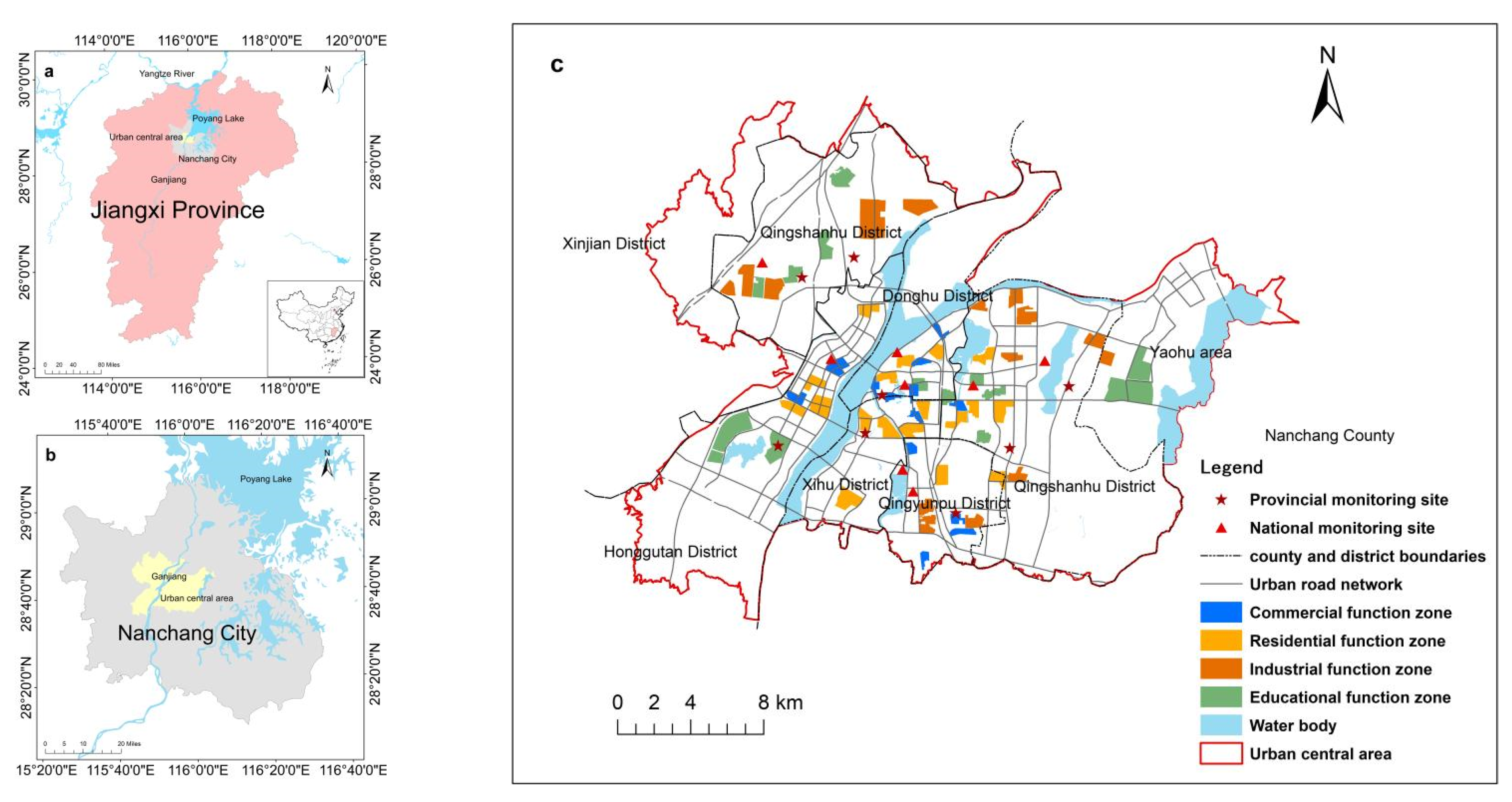
2.1. Study Area
2.2. Data Sources and Methods
2.2.1. Data Sources
2.2.2. Identification of Urban Land-Use Function Zones
2.2.3. The 3D Landscape Indices Adopted
2.2.4. LUR Modeling
2.2.5. Impact of 3D Landscape Pattern on PM2.5
3. Results
3.1. Distribution of Land-Use Function Zones
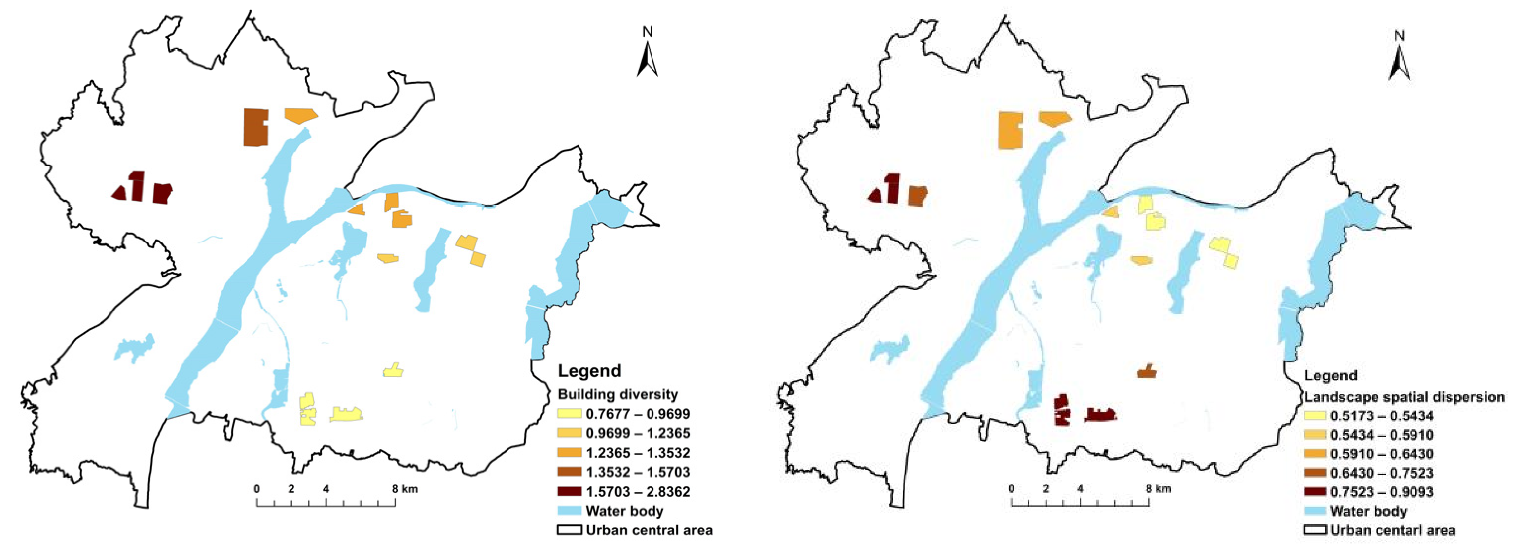
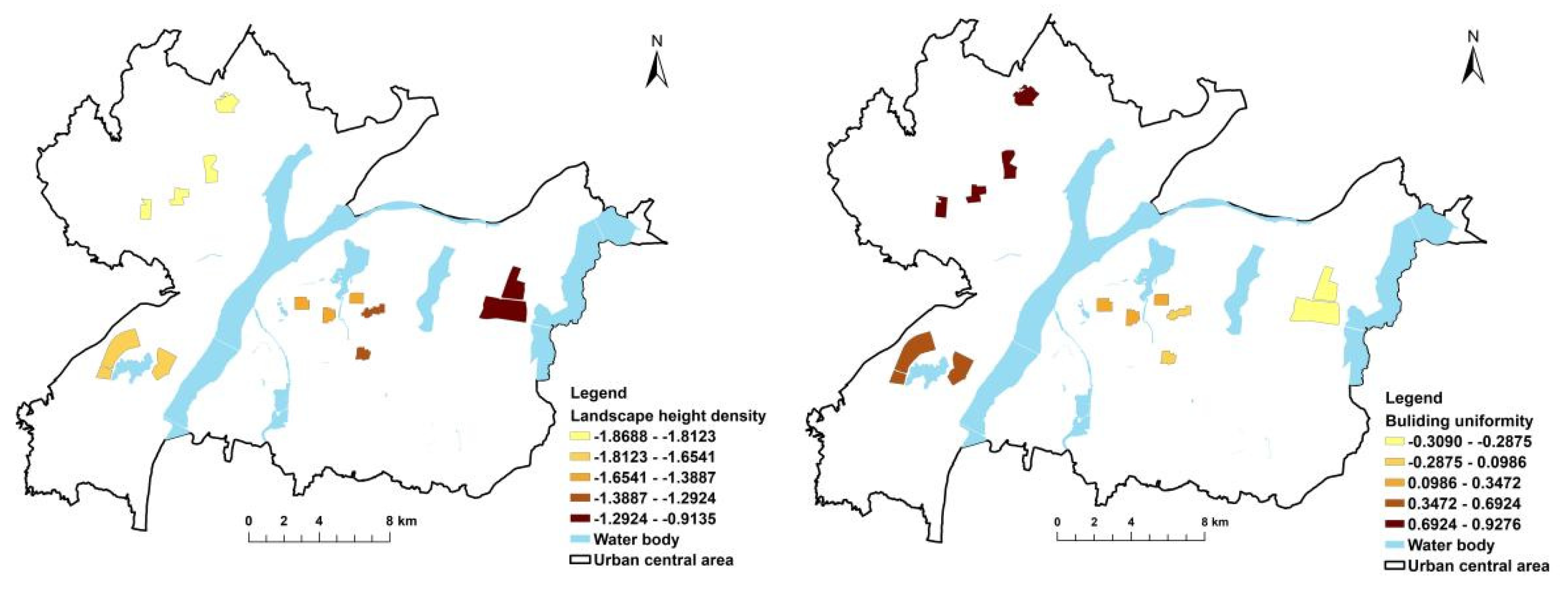
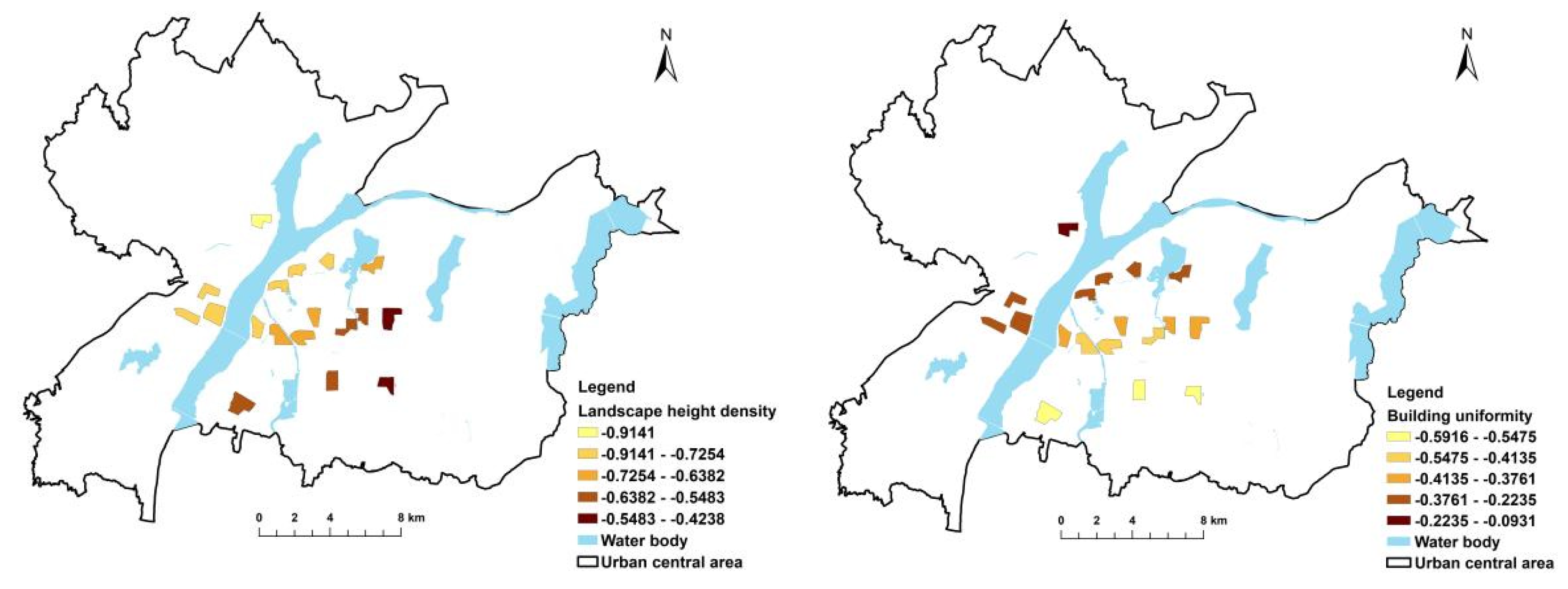
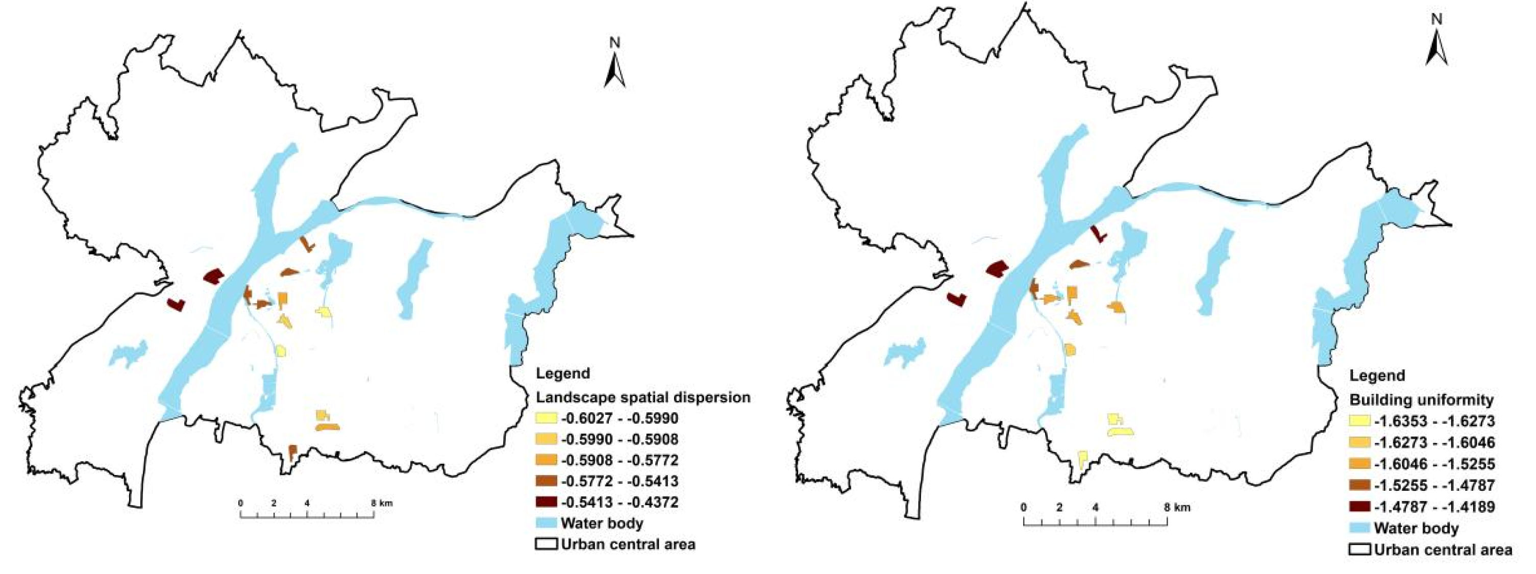
3.2. The 3D Characteristics of Land-Use Function Zone
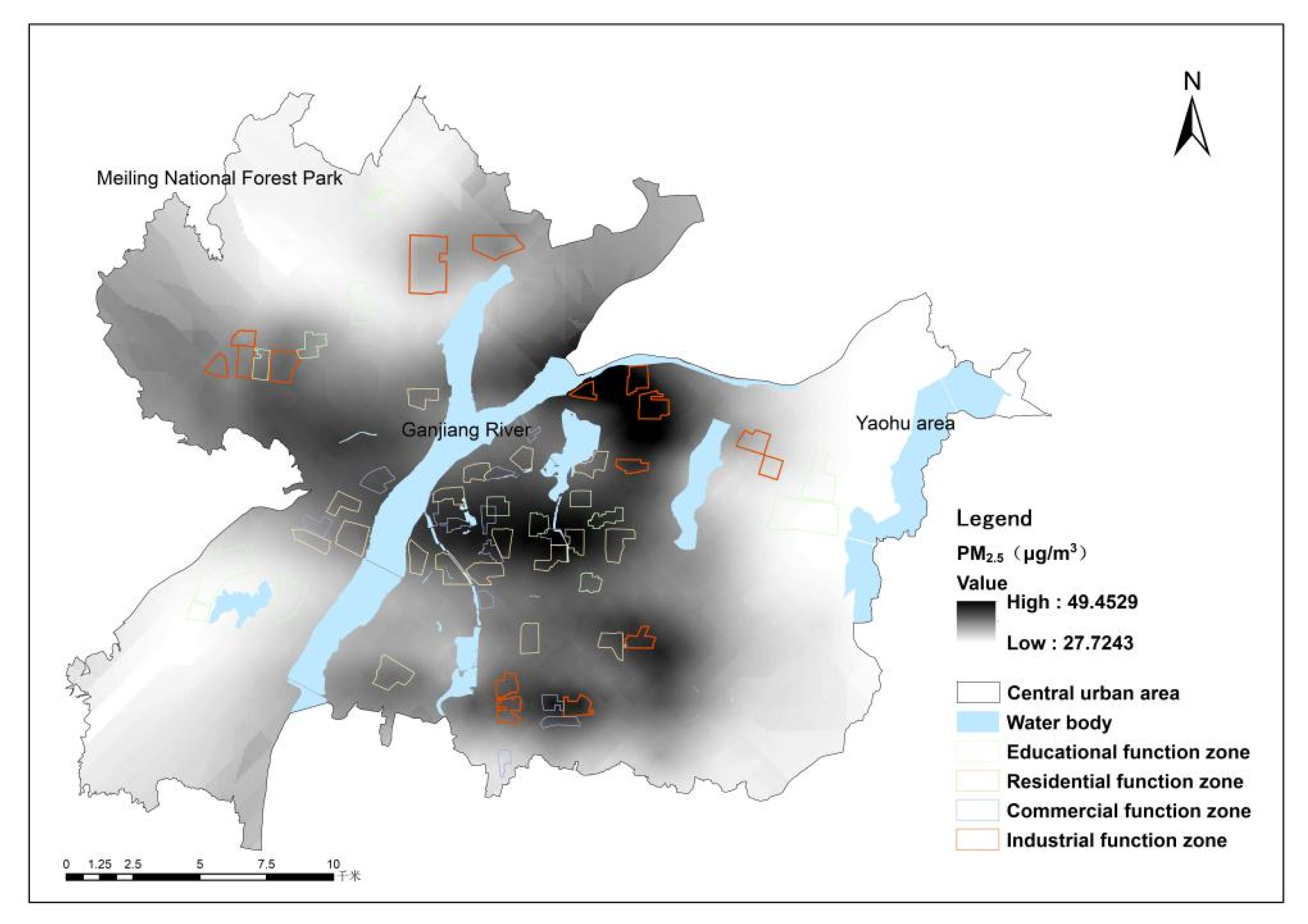
3.3. Spatial Heterogeneity of PM2.5 Using LUR Model
3.4. Inference of 3D Indices on PM2.5 in Different Land Function Zones
3.5. The Spatial Variance of 3D Indices Using GWR Model
4. Discussion
5. Conclusions
Author Contributions
Funding
Institutional Review Board Statement
Informed Consent Statement
Data Availability Statement
Conflicts of Interest
References
- Pan Jiahua, P.; Jingjing, S.; Zhanyun, W. Blue Book of Cities in China: Annual Report on Urban Development of CHINA NO.12; Social Science Academic Press: Beijing, China, 2019. [Google Scholar]
- She, Q.; Peng, X.; Xu, Q.; Long, L.; Wei, N.; Liu, M.; Xiang, W. Air quality and its response to satellite-derived urban form in the Yangtze River Delta, China. Ecol. Indic. 2017, 75, 75297–75306. [Google Scholar] [CrossRef]
- Chen, G.; Li, S.; Knibbs, L.D.; Hamm, N.A.S.; Cao, W.; Li, T.; Guo, J.; Ren, H.; Abramson, M.J.; Guo, Y. A machine learning method to estimate PM2.5 concentrations across China with remote sensing, meteorological and land use information. Sci. Total Environ. 2018, 636, 52–60. [Google Scholar] [CrossRef]
- Xu, H.; Bechle, M.J.; Wang, M.; Szpiro, A.A.; Vedal, S.; Bai, Y.; Marshall, J.D. National PM2.5 and NO2 exposure models for China based on land use regression, satellite measurements, and universal kriging. Sci. Total Environ. 2018, 655, 423–433. [Google Scholar] [CrossRef] [PubMed]
- Erqou, S.; Clougherty, J.E.; Olafiranye, O.; Magnani, J.W.; Aiyer, A.; Tripathy, S.; Reis, S.E. Particulate Matter Air Pollution and Racial Differences in Cardiovascular Disease Risk. Arterioscler. Thromb. Vasc. Biol. 2018, 38, 935–942. [Google Scholar] [CrossRef] [PubMed]
- Pope, C.A., III; Burnett, R.T.; Thun, M.J.; Calle, E.E.; Krewski, D.; Ito, K.; Thurston, G.D. Lung cancer, cardiopulmonary mortality, and long-term exposure to fine particulate air pollution. JAMA 2002, 287, 1132–1141. [Google Scholar] [CrossRef]
- Thiankhaw, K.; Chattipakorn, N.; Chattipakorn, S.C. PM2.5 exposure in association with AD-related neuropathology and cognitive outcomes. Environ. Pollut. 2021, 292, 118320. [Google Scholar] [CrossRef]
- Han, L.; Zhou, W.; Pickett, S.T.A.; Li, W.; Qian, Y. Risks and Causes of Population Exposure to Cumulative Fine Particulate (PM2.5) Pollution in China. Earth’s Futur. 2019, 7, 615–622. [Google Scholar] [CrossRef]
- Wu, J.; Zhang, P.; Yi, H.; Qin, Z. What Causes Haze Pollution? An Empirical Study of PM2.5 Concentrations in Chinese Cities. Sustainability 2016, 8, 132. [Google Scholar] [CrossRef]
- Li, Y.; Chen, Q.; Zhao, H.; Wang, L.; Tao, R. Variations in PM10, PM2.5 and PM1.0 in an urban area of the Sichuan Basin and their relation to meteorological factors. Atmosphere 2015, 6, 150–163. [Google Scholar] [CrossRef]
- Guo, J.; Xia, F.; Zhang, Y.; Liu, H.; Li, J.; Lou, M.; Zhai, P. Impact of diurnal variability and meteorological factors on the PM2.5—AOD relationship: Implications for PM2.5 remote sensing. Environ. Pollut. 2017, 221, 94–104. [Google Scholar] [CrossRef]
- Amini, H.; Taghavi-Shahri, S.M.; Henderson, S.B.; Naddafi, K.; Nabizadeh, R.; Yunesian, M. Land use regression models to estimate the annual and seasonal spatial variability of sulfur dioxide and particulate matter in Tehran, Iran. Sci. Total Environ. 2014, 488–489, 343–353. [Google Scholar] [CrossRef] [PubMed]
- Fu, B.; Liang, D.; Lu, N. Landscape ecology: Coupling of pattern, process, and scale. Chin. Geogr. Sci. 2011, 21, 385. [Google Scholar] [CrossRef]
- Shi, Y.; Ren, C.; Lau, K.K.L.; Ng, E. Investigating the influence of urban land use and landscape pattern on PM2.5 spatial variation using mobile monitoring and WUDAPT. Landsc. Urban Plan. 2019, 189, 15–26. [Google Scholar] [CrossRef]
- Lu, D.; Mao, W.; Yang, D.; Zhao, J.; Xu, J. Effects of land use and landscape pattern on PM2.5 in Yangtze River Delta, China. Atmos. Pollut. Res. 2018, 9, 705–713. [Google Scholar] [CrossRef]
- Sun, L.; Wei, J.; Duan, D.H.; Guo, Y.M.; Yang, D.X.; Jia, C.; Mi, X.T. Impact of Land-Use and Land-Cover Change on urban air quality in representative cities of China. J. Atmos. Sol.-Terr. Phys. 2016, 142, 43–54. [Google Scholar] [CrossRef]
- Saraswat, A.; Apte, J.S.; Kandlikar, M.; Brauer, M.; Henderson, S.B.; Marshall, J.D. Spatiotemporal Land Use Regression Models of Fine, Ultrafine, and Black Carbon Particulate Matter in New Delhi, India. Environ. Sci. Technol. 2013, 47, 12903–12911. [Google Scholar] [CrossRef]
- Zhai, H.; Yao, J.; Wang, G.; Tang, X. Impact of Land Use on Atmospheric Particulate Matter Concentrations: A Case Study of the Beijing–Tianjin–Hebei Region, China. Atmosphere 2022, 13, 391. [Google Scholar] [CrossRef]
- Shao, J.; Ge, J.; Feng, X.; Zhao, C. Study on the relationship between PM2.5 concentration and intensive land use in Hebei Province based on a spatial regression model. PLoS ONE 2020, 15, e0238547. [Google Scholar] [CrossRef]
- Yang, H.; Chen, W.; Liang, Z. Impact of Land Use on PM2.5 Pollution in a Representative City of Middle China. Int. J. Environ. Res. Public Health 2017, 14, 462. [Google Scholar] [CrossRef]
- Ke, B.; Hu, W.; Huang, D.; Zhang, J.; Lin, X.; Li, C.; Jin, X.; Chen, J. Three-dimensional building morphology impacts on PM2.5 distribution in urban landscape settings in Zhejiang, China. Sci. Total Environ. 2022, 826, 154094. [Google Scholar] [CrossRef]
- Liu, Y.; He, L.; Qin, W.; Lin, A.; Yang, Y. The Effect of Urban Form on PM2.5 Concentration: Evidence from China’s 340 Pre-fecture-Level Cities. Remote Sens. 2021, 14, 7. [Google Scholar] [CrossRef]
- Zou, B.; Fang, X.; Feng, H.; Zhou, X. Simplicity versus accuracy for estimation of the PM2.5 concentration: A comparison between LUR and GWR methods across time scales. J. Spat. Sci. 2019, 66, 279–297. [Google Scholar] [CrossRef]
- Tian, Y.; Zhou, W.; Qian, Y.; Zheng, Z.; Yan, J. The effect of urban 2D and 3D morphology on air temperature in residential neighborhoods. Landsc. Ecol. 2019, 34, 1161–1178. [Google Scholar] [CrossRef]
- Wu, Q.; Guo, F.; Li, H.; Kang, J. Measuring landscape pattern in three dimensional space. Landsc. Urban Plan. 2017, 167, 49–59. [Google Scholar] [CrossRef]
- Kedron, P.; Zhao, Y.; Frazier, A.E. Three dimensional (3D) spatial metrics for objects. Landsc. Ecol. 2019, 34, 2123–2132. [Google Scholar] [CrossRef]
- Liu, M.; Hu, Y.M.; Li, C.L. Landscape metrics for three-dimensional urban building pattern recognition. Appl. Geogr. 2017, 87, 66–72. [Google Scholar] [CrossRef]
- Xu, Y.; Liu, M.; Hu, Y.; Li, C.; Xiong, Z. Analysis of Three-Dimensional Space Expansion Characteristics in Old Industrial Area Renewal Using GIS and Barista: A Case Study of Tiexi District, Shenyang, China. Sustainability 2019, 11, 1860. [Google Scholar] [CrossRef]
- Edussuriya, P.; Chan, A.; Ye, A. Urban morphology and air quality in dense residential environments in Hong Kong. Part I: District-level analysis. Atmos. Environ. 2011, 45, 4789–4803. [Google Scholar] [CrossRef]
- Yang, F.; Qian, F.; Lau, S.S. Urban form and density as indicators for summertime outdoor ventilation potential: A case study on high-rise housing in Shanghai. Build. Environ. 2013, 70, 122–137. [Google Scholar] [CrossRef]
- Cai, H.; Xu, X. Impacts of built-up area expansion in 2D and 3D on regional surface temperature. Sustainability 2017, 9, 1862. [Google Scholar] [CrossRef]
- Vienneau, D.; De Hoogh, K.; Beelen, R.; Fischer, P.; Hoek, G.; Briggs, D. Comparison of land-use regression models between Great Britain and the Netherlands. Atmos. Environ. 2010, 44, 688–696. [Google Scholar] [CrossRef]
- Hogg, R.V.; Ledolter, J. Engineering Statistics; Macmillan Pub. Co.: New York, NY, USA, 1987. [Google Scholar]
- McHugh, M.L. Multiple comparison analysis testing in ANOVA. Biochem. Med. 2011, 21, 203–209. [Google Scholar] [CrossRef] [PubMed]
- Marshall, J.D.; Nethery, E.; Brauer, M. Within-urban variability in ambient air pollution: Comparison of estimation methods. Atmos. Environ. 2008, 42, 1359–1369. [Google Scholar] [CrossRef]
- Lu, T.; Bechle, M.J.; Wan, Y.; Presto, A.A.; Hankey, S. Using crowd-sourced low-cost sensors in a land use regression of PM2.5 in 6 US cities. Air Qual. Atmos. Health 2022, 15, 667–678. [Google Scholar] [CrossRef]
- Hoek, G.; Beelen, R.; De Hoogh, K.; Vienneau, D.; Gulliver, J.; Fischer, P.; Briggs, D. A review of land-use regression models to assess spatial variation of outdoor air pollution. Atmos. Environ. 2008, 42, 7561–7578. [Google Scholar] [CrossRef]
- Henderson, S.B.; Beckerman, B.; Jerrett, M.; Brauer, M. Application of Land Use Regression to Estimate Long-Term Concentrations of Traffic-Related Nitrogen Oxides and Fine Particulate Matter. Environ. Sci. Technol. 2007, 41, 2422–2428. [Google Scholar] [CrossRef]
- Zhang, P.; Yang, L.; Ma, W.; Wang, N.; Wen, F.; Liu, Q. Spatiotemporal estimation of the PM2.5 concentration and human health risks combining the three-dimensional landscape pattern index and machine learning methods to optimize land use regression modeling in Shaanxi, China. Environ. Res. 2022, 208, 112759. [Google Scholar] [CrossRef]
- Li, K.; Li, C.; Liu, M.; Hu, Y.; Wang, H.; Wu, W. Multiscale analysis of the effects of urban green infrastructure landscape patterns on PM2.5 concentrations in an area of rapid urbanization. J. Clean. Prod. 2021, 325, 129324. [Google Scholar] [CrossRef]
- Zhang, T.; Gong, W.; Wang, W.; Ji, Y.; Zhu, Z.; Huang, Y. Ground Level PM2.5 Estimates over China Using Satellite-Based Geographically Weighted Regression (GWR) Models Are Improved by Including NO2 and Enhanced Vegetation Index (EVI). Int. J. Environ. Res. Public Health 2016, 13, 1215. [Google Scholar] [CrossRef]
- Song, W.; Jia, H.; Huang, J.; Zhang, Y. A satellite-based geographically weighted regression model for regional PM2.5 estimation over the Pearl River Delta region in China. Remote Sens. Environ. 2014, 154, 1–7. [Google Scholar] [CrossRef]
- McMillen, D.P. Geographically Weighted Regression: The Analysis of Spatially Varying Relationships. Am. J. Agric. Econ. 2004, 86, 554–556. [Google Scholar] [CrossRef]
- Du Preez, C. A new arc–chord ratio (ACR) rugosity index for quantifying three-dimensional landscape structural complexity. Landsc. Ecol. 2015, 30, 181–192. [Google Scholar] [CrossRef]
- Liu, X.; Peng, W. Urban functional zoning and zoning classification management. Urban Oper. Manag. 2010, 4, 20–22. [Google Scholar]
- Son, Y.; Osornio-Vargas, R.; O’Neill, M.S.; Hystad, P.; Texcalac-Sangrador, J.L.; Ohman-Strickland, P.; Meng, Q.; Schwander, S. Land use regression models to assess air pollution exposure in Mexico City using finer spatial and temporal input parameters. Sci. Total Environ. 2018, 639, 40–48. [Google Scholar] [CrossRef]
- Zhang, L.; Tian, X.; Zhao, Y.; Liu, L.; Li, Z.; Tao, L.; Wang, X.; Guo, X.; Luo, Y. Application of nonlinear land use regression models for ambient air pollutants and air quality index. Atmos. Pollut. Res. 2021, 12, 101186. [Google Scholar] [CrossRef]
- Huang, L.; Zhang, C.; Bi, J. Development of land use regression models for PM2.5, SO2, NO2 and O3 in Nanjing, China. Environ. Res. 2017, 158, 542–552. [Google Scholar] [CrossRef]
- Douglas, A.N.; Irga, P.J.; Torpy, F.R. Determining broad scale associations between air pollutants and urban forestry: A novel multifaceted methodological approach. Environ. Pollut. 2019, 247, 474–481. [Google Scholar] [CrossRef]
- Tularam, H.; Ramsay, L.; Muttoo, S.; Naidoo, R.; Brunekreef, B.; Meliefste, K.; De Hoogh, K. Harbor and Intra-City Drivers of Air Pollution: Findings from a Land Use Regression Model, Durban, South Africa. Int. J. Environ. Res. Public Health 2020, 17, 5406. [Google Scholar] [CrossRef]
- Chen, L.; Wu, Z.; Tu, W.; Cao, Z. Applying LUR Model to Estimate Spatial Variation of PM2.5 in the Greater Bay Area, China. Spatiotemporal Analysis of Air Pollution and Its Application in Public Health; Elsevier: Amsterdam, The Netherlands, 2020; pp. 207–215. [Google Scholar]
- Liu, T.; Xiao, J.; Zeng, W.; Hu, J.; Liu, X.; Dong, M.; Ma, W. A spatiotemporal land-use-regression model to assess individual level long-term exposure to ambient fine particulate matters. MethodsX 2019, 6, 2101. [Google Scholar] [CrossRef]
- Wu, C.D.; Chen, Y.C.; Pan, W.C.; Zeng, Y.T.; Chen, M.J.; Guo, Y.L.; Lung, S.C.C. Land-use regression with long-term satellite-based greenness index and culture-specific sources to model PM2.5 spatial-temporal variability. Environ. Pollut. 2017, 224, 148–157. [Google Scholar] [CrossRef]
- Chan, L.Y.; Kwok, W.S. Vertical dispersion of suspended particulates in urban area of Hong Kong. Atmos. Environ. 2000, 34, 4403–4412. [Google Scholar] [CrossRef]
- Huang, Y.; Shen, H.; Chen, H.; Wang, R.; Zhang, Y.; Su, S.; Tao, S. Quantification of Global Primary Emissions of PM2.5, PM10, and TSP from Com-bustion and Industrial Process Sources. Environ. Sci. Technol. 2014, 48, 13834–13843. [Google Scholar] [CrossRef] [PubMed]
- Chen, Y.-C.; Fröhlich, D.; Matzarakis, A.; Lin, T.-P. Urban Roughness Estimation Based on Digital Building Models for Urban Wind and Thermal Condition Estimation—Application of the SkyHelios Model. Atmosphere 2017, 8, 247. [Google Scholar] [CrossRef]


| 3D Feature | Schematic Diagram | Methods Description |
|---|---|---|
| Height |   | Height is the most basic and intuitive feature that distinguishes 3D space from the 2D plane. It can be reflected by the average value of building height. |
| Congestion |   | Congestion denotes the density of buildings in the sample area. The different volume, shape, floor area, and peripheral outline of urban buildings will affect the architectural landscape pattern of the area. The openness of buildings plays an important role in atmospheric diffusion. The degree of congestion can be calculated from the ratio of the sum of the building volume and the maximum height of the building multiplied by the area of the sample area. |
| Fluctuation |  | Fluctuation shows the difference in the building height in the sample area. The fluctuation feature is also a basic indicator to describe the 3D feature of the landscape. It can be calculated from the difference between the highest value and the lowest value of the building height in the sample area. |
| Diversity |   | Diversity indicates the number of buildings with different heights in the sample area. The diversity index in the 2D plane is often used to calculate the heterogeneity of the community. In the 3D environment, after dividing the building into different categories according to height, the spatial characteristics can be measured from the spatial heterogeneity. The buildings are divided into different categories according to their height, and the heterogeneity of the architectural landscape can be calculated using the Shannonville diversity index and uniformity index. |
| 3D Feature | 3D Landscape Index | Formula | Description |
|---|---|---|---|
| Height | Landscape height density | Representing the average height of the architectural landscape. Hi is the height of building i, and n is the number of buildings in the sample area. | |
| Congestion | Landscape volume density | Vi is the volume of building i, is the maximum height of the building in the sample area, and S is the area of the sample area. | |
| Fluctuation | Landscape spatial dispersion | Representing the degree of dispersion of building height. Hi is the height of building i. | |
| Landscape fluctuation | is the maximum building height in the landscape, and is the minimum building height in the landscape. | ||
| Diversity | Building diversity | Pi is the percentage of the area occupied by buildings of type i, and m is the total number of building types in the landscape. | |
| Building uniformity | Representing the uniformity of building distribution. is the maximum diversity index in the landscape. |
| Factor | Variable | Description | Unit | Assumed Correlation |
|---|---|---|---|---|
| Road | MROAD | Proportion of main road length to buffer area | m | + |
| SROAD | Proportion of secondary road length to buffer area | m | + | |
| TAL | Proportion of total road length to buffer area | m | + | |
| Land use | VEG | Proportion of ecological area (forest, water, etc.) to buffer area | % | − |
| INDU | Proportion of industrial land area to buffer area | % | + | |
| WAT | Proportion of water area to buffer area | % | − | |
| RAR | Proportion of arable land area to buffer area | % | −−−− | |
| Population | POP | Proportion of residential land area to buffer area | % | + |
| Meteorological factor | PRS | Air pressure | hPa | −−−− |
| PRS_Sea | Sea pressure | hPa | −−−− | |
| WIN | Wind speed | m/s | −−−− | |
| TEM | Temperature | °C | −−−− | |
| RHU | Relative humidity | % | −−−− | |
| PRE_1 h | Hourly precipitation | mm | −−−− |
| Type | Number | Max (km2) | Min (km2) | Mean (km2) |
|---|---|---|---|---|
| Industrial function zone | 16 | 2.88 | 0.37 | 0.84 |
| Educational function zone | 14 | 2.93 | 0.40 | 1.05 |
| Residential function zone | 18 | 1.13 | 0.50 | 0.70 |
| Commercial function zone | 13 | 0.73 | 0.31 | 0.39 |
| Variable | Type III Sum of Squares | Degree of Freedom | Mean Square | F | Significance |
|---|---|---|---|---|---|
| Landscape height density | 344.637 | 3 | 114.879 | 5.253 | 0.003 |
| Landscape volume density | 31.167 | 3 | 10.389 | 6.993 | 0.000 |
| Landscape spatial dispersion | 1.085 | 3 | 0.362 | 5.082 | 0.003 |
| Landscape fluctuation | 16,998.259 | 3 | 5666.086 | 11.356 | 0.000 |
| Building diversity | 1.933 | 3 | 0.644 | 4.116 | 0.010 |
| Building uniformity | 1.027 | 3 | 0.136 | 3.894 | 0.015 |
| Variable | Function Zone (I) | Function Zone (J) | Mean Difference | Standard Error | Significance |
|---|---|---|---|---|---|
| Landscape height density | Commercial | Residential | −0.996 | 1.702 | 0.561 |
| Educational | −0.362 | 1.772 | 0.839 | ||
| Industrial | 4.818 * | 1.746 | 0.008 | ||
| Residential | Commercial | 0.996 | 1.702 | 0.561 | |
| Educational | 0.635 | 1.635 | 0.699 | ||
| Industrial | 5.814 * | 1.607 | 0.001 | ||
| Educational | Commercial | 0.362 | 1.772 | 0.839 | |
| Residential | −0.635 | 1.635 | 0.699 | ||
| Industrial | 5.179 * | 1.681 | 0.003 | ||
| Industrial | Commercial | −4.818 * | 1.746 | 0.008 | |
| Residential | −5.814 * | 1.607 | 0.001 | ||
| Educational | −5.179 * | 1.681 | 0.003 | ||
| Landscape volume density | Commercial | Residential | 0.378 | 0.444 | 0.398 |
| Educational | 1.758 * | 0.462 | 0.000 | ||
| Industrial | 1.441 * | 0.455 | 0.002 | ||
| Residential | Commercial | −0.378 | 0.444 | 0.398 | |
| Educational | 1.381 * | 0.426 | 0.002 | ||
| Industrial | 1.063 * | 0.419 | 0.014 | ||
| Educational | Commercial | −1.758 * | 0.462 | 0.000 | |
| Residential | −1.381 * | 0.426 | 0.002 | ||
| Industrial | −0.318 | 0.438 | 0.471 | ||
| Industrial | Commercial | −1.441 * | 0.455 | 0.002 | |
| Residential | −1.063 * | 0.419 | 0.014 | ||
| Educational | 0.318 | 0.438 | 0.471 | ||
| Landscape spatial dispersion | Commercial | Residential | 0.017 | 0.097 | 0.860 |
| Educational | 0.230 * | 0.101 | 0.027 | ||
| Industrial | 0.305 * | 0.100 | 0.003 | ||
| Residential | Commercial | −0.017 | 0.097 | 0.860 | |
| Educational | 0.213 * | 0.093 | 0.026 | ||
| Industrial | 0.288 * | 0.092 | 0.003 | ||
| Educational | Commercial | −0.230 * | 0.101 | 0.027 | |
| Residential | −0.213 * | 0.093 | 0.026 | ||
| Industrial | 0.076 | 0.096 | 0.434 | ||
| Industrial | Commercial | −0.305 * | 0.100 | 0.003 | |
| Residential | −0.288 * | 0.092 | 0.003 | ||
| Educational | −0.076 | 0.096 | 0.434 | ||
| Landscape fluctuation | Commercial | Residential | −2.874 | 8.130 | 0.725 |
| Educational | 20.055 * | 8.464 | 0.021 | ||
| Industrial | 37.428 * | 8.341 | 0.000 | ||
| Residential | Commercial | 2.874 | 8.130 | 0.725 | |
| Educational | 22.929 * | 7.809 | 0.005 | ||
| Industrial | 40.301 * | 7.675 | 0.000 | ||
| Educational | Commercial | −20.055 * | 8.464 | 0.021 | |
| Residential | −22.930 * | 7.809 | 0.005 | ||
| Industrial | 17.372 * | 8.028 | 0.035 | ||
| Industrial | Commercial | −37.428 * | 8.341 | 0.000 | |
| Residential | −40.301 * | 7.675 | 0.000 | ||
| Educational | −17.372 * | 8.028 | 0.035 | ||
| Building diversity | Commercial | Residential | 0.027 | 0.144 | 0.852 |
| Educational | 0.176 | 0.150 | 0.246 | ||
| Industrial | 0.443 * | 0.148 | 0.004 | ||
| Residential | Commercial | −0.027 | 0.144 | 0.852 | |
| Educational | 0.149 | 0.138 | 0.287 | ||
| Industrial | 0.416 * | 0.136 | 0.003 | ||
| Educational | Commercial | −0.176 | 0.150 | 0.246 | |
| Residential | −0.149 | 0.138 | 0.287 | ||
| Industrial | 0.267 | 0.142 | 0.065 | ||
| Industrial | Commercial | −0.443 * | 0.148 | 0.004 | |
| Residential | −0.416 * | 0.136 | 0.003 | ||
| Educational | −0.267 | 0.142 | 0.065 | ||
| Building uniformity | Commercial | Residential | 0.022 * | 0.079 | 0.059 |
| Educational | 0.016 | 0.082 | 0.158 | ||
| Industrial | 0.151 * | 0.081 | 0.003 | ||
| Residential | Commercial | −0.022 | 0.079 | 0.059 | |
| Educational | −0.006 | 0.076 | 0.227 | ||
| Industrial | 0.129 * | 0.075 | 0.001 | ||
| Educational | Commercial | −0.016 | 0.082 | 0.158 | |
| Residential | 0.006 | 0.076 | 0.227 | ||
| Industrial | 0.135 * | 0.078 | 0.050 | ||
| Industrial | Commercial | −0.151 | 0.081 | 0.003 | |
| Residential | −0.129 * | 0.075 | 0.001 | ||
| Educational | −0.135 * | 0.078 | 0.050 |
| Variable | Land Use Regression Model | Goodness of Fit (R2) | Adjusted R2 | Average Absolute Error Rate | RMSE |
|---|---|---|---|---|---|
| PM2.5 | Y = 41.308 − 5.921XVEG5000 + 40.316XPRE − 26.102XPRS_Sea + 4.088XINDU500 | 0.958 | 0.917 | 0.094 | 4.583 |
| 3D Landscape Index | Industrial Function Zone | Educational Function Zone | Residential Function Zone | Commercial Function Zone |
|---|---|---|---|---|
| Landscape height density | 0.518 * | −0.556 * | −0.546 * | −0.061 |
| Landscape volume density | 0.048 | 0.325 | −0.095 | −0.270 |
| Landscape spatial dispersion | 0.342 | 0.112 | −0.051 | −0.574 * |
| Landscape undulation | 0.454 | −0.262 | −0.263 | −0.473 |
| Building diversity | 0.589 * | −0.211 | −0.304 | −0.602 * |
| Building uniformity | 0.482 * | 0.108 | −0.358 | −0.635 * |
| Variable | Goodness of Fit (R2) | Adjusted R2 | Moran’s Index | p-Value |
|---|---|---|---|---|
| Industrial function zone | 0.8832 | 0.7145 | 0.1181 | 0.3431 |
| Commercial function zone | 0.7938 | 0.6852 | 0.0123 | 0.6876 |
| Educational function zone | 0.5295 | 0.4569 | −0.2052 | 0.4625 |
| Residential function zone | 0.3129 | 0.2145 | 0.1440 | 0.3091 |
Publisher’s Note: MDPI stays neutral with regard to jurisdictional claims in published maps and institutional affiliations. |
© 2022 by the authors. Licensee MDPI, Basel, Switzerland. This article is an open access article distributed under the terms and conditions of the Creative Commons Attribution (CC BY) license (https://creativecommons.org/licenses/by/4.0/).
Share and Cite
Chen, W.; Zhang, F.; Luo, S.; Lu, T.; Zheng, J.; He, L. Three-Dimensional Landscape Pattern Characteristics of Land Function Zones and Their Influence on PM2.5 Based on LUR Model in the Central Urban Area of Nanchang City, China. Int. J. Environ. Res. Public Health 2022, 19, 11696. https://doi.org/10.3390/ijerph191811696
Chen W, Zhang F, Luo S, Lu T, Zheng J, He L. Three-Dimensional Landscape Pattern Characteristics of Land Function Zones and Their Influence on PM2.5 Based on LUR Model in the Central Urban Area of Nanchang City, China. International Journal of Environmental Research and Public Health. 2022; 19(18):11696. https://doi.org/10.3390/ijerph191811696
Chicago/Turabian StyleChen, Wenbo, Fuqing Zhang, Saiwei Luo, Taojie Lu, Jiao Zheng, and Lei He. 2022. "Three-Dimensional Landscape Pattern Characteristics of Land Function Zones and Their Influence on PM2.5 Based on LUR Model in the Central Urban Area of Nanchang City, China" International Journal of Environmental Research and Public Health 19, no. 18: 11696. https://doi.org/10.3390/ijerph191811696
APA StyleChen, W., Zhang, F., Luo, S., Lu, T., Zheng, J., & He, L. (2022). Three-Dimensional Landscape Pattern Characteristics of Land Function Zones and Their Influence on PM2.5 Based on LUR Model in the Central Urban Area of Nanchang City, China. International Journal of Environmental Research and Public Health, 19(18), 11696. https://doi.org/10.3390/ijerph191811696