

Analysis of Air and Soil Quality around Thermal Power Plants and Coal Mines of Singrauli Region, India


Abstract
:1. Introduction
2. Materials and Methods
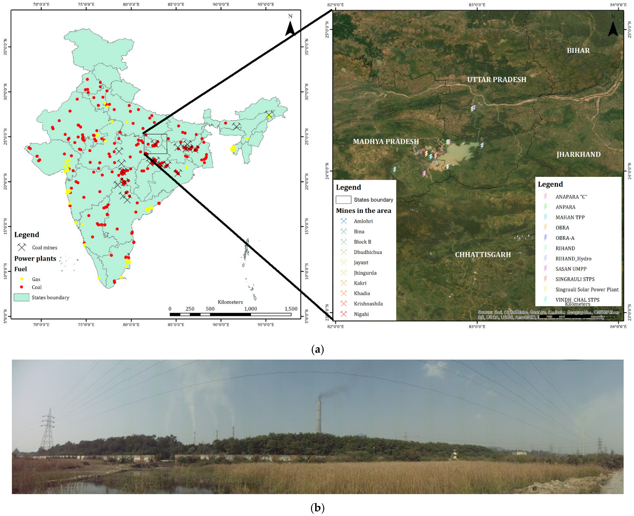
2.1. Study Area
2.2. Materials
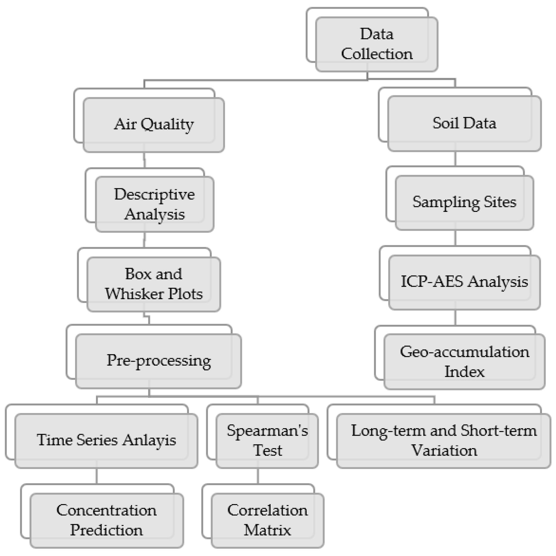
2.3. Methods
2.3.1. Air Quality Analysis
2.3.2. Soil Quality Analysis
3. Results
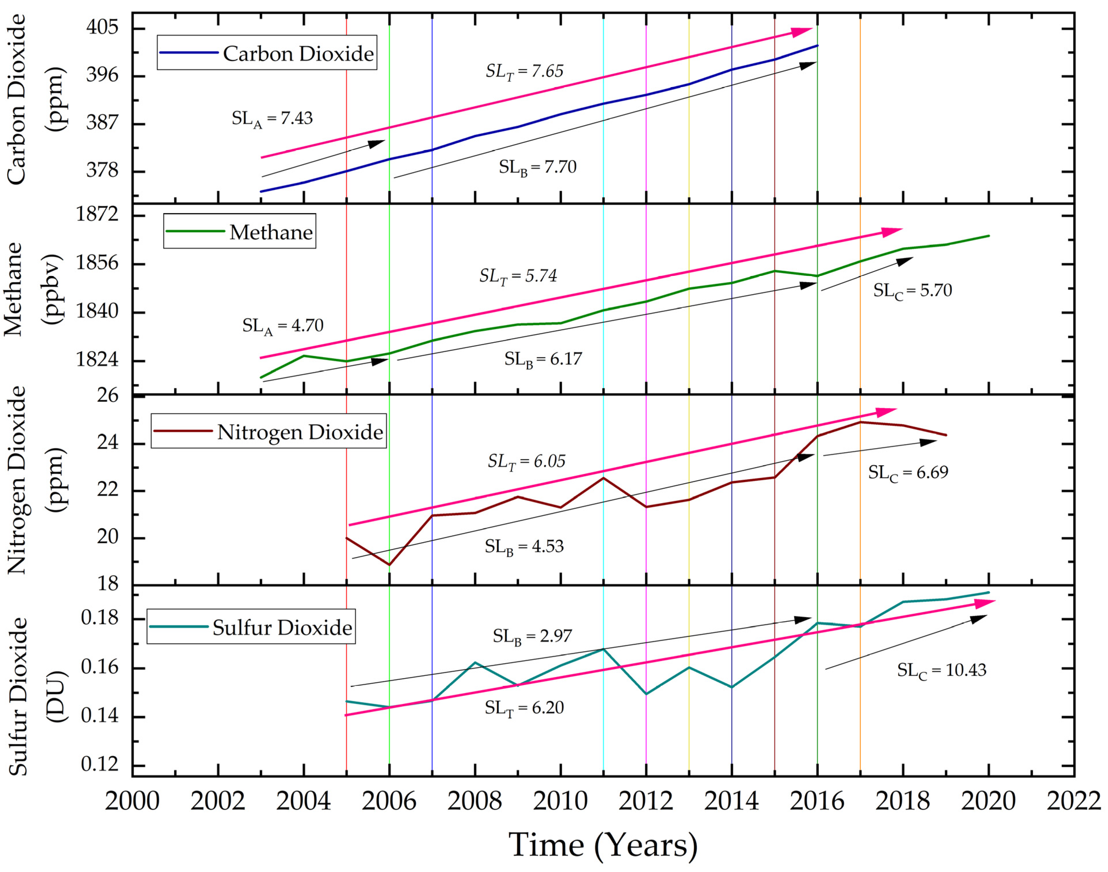
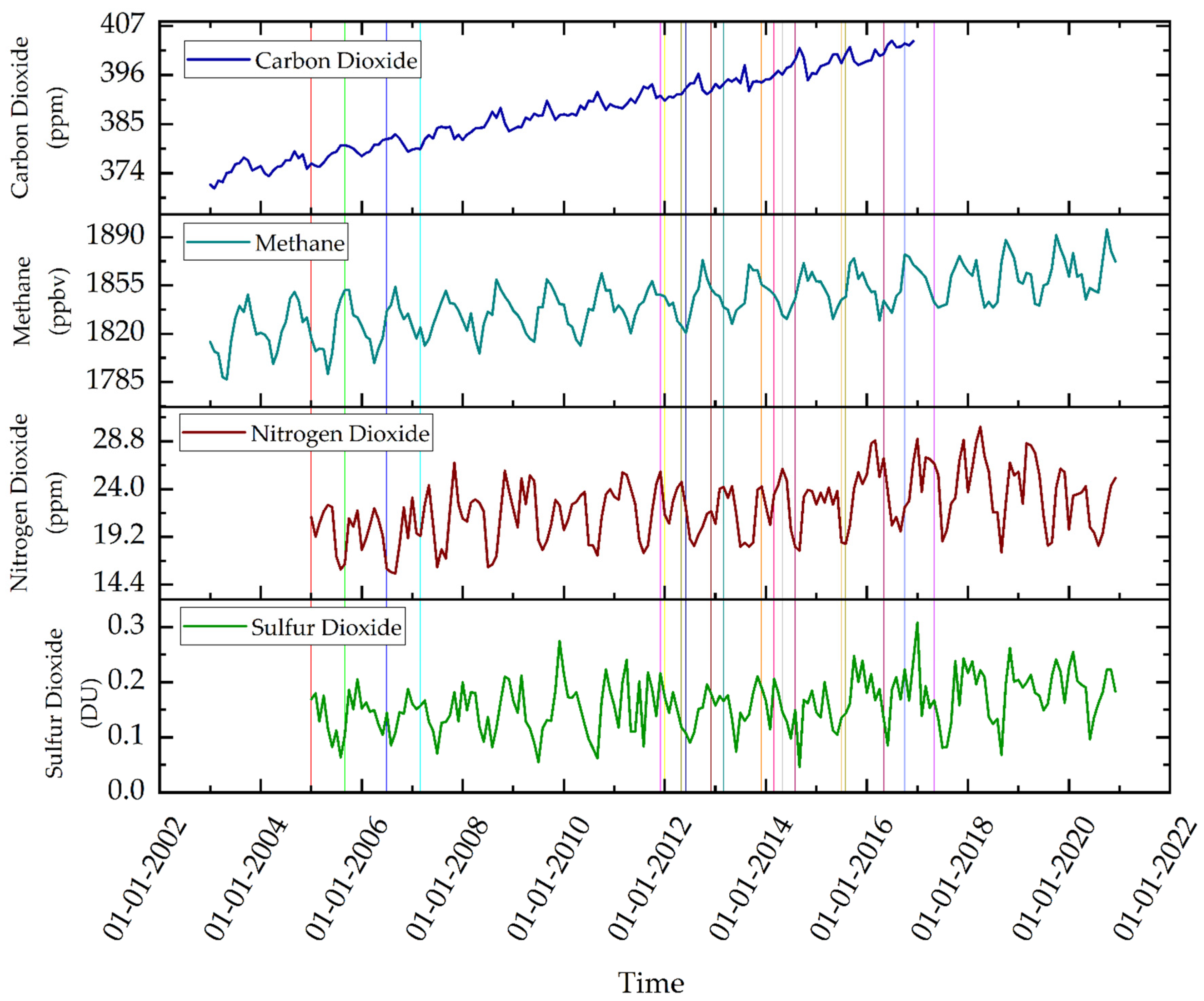
3.1. Long-Term Variations of Pollutants Associated with Thermal Power Plants
3.2. Short-Term Variation of Pollutants Associated with the Thermal Power Plants
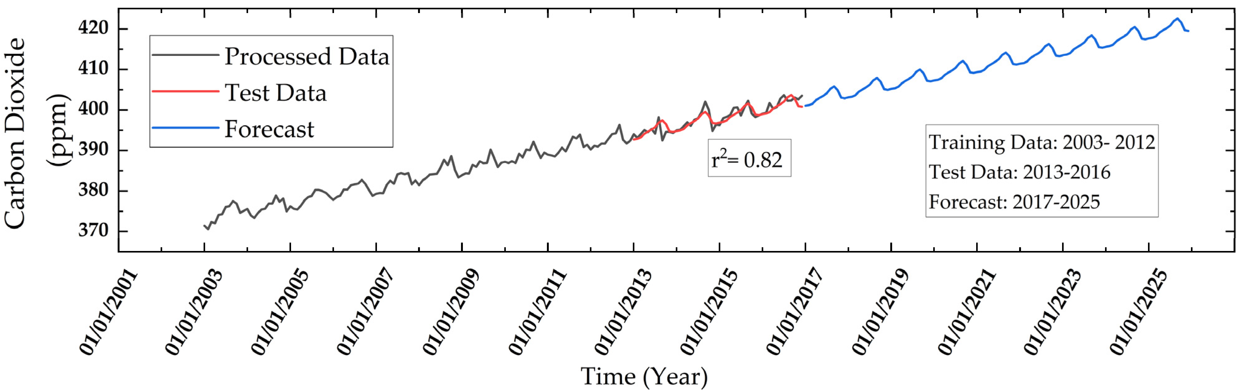
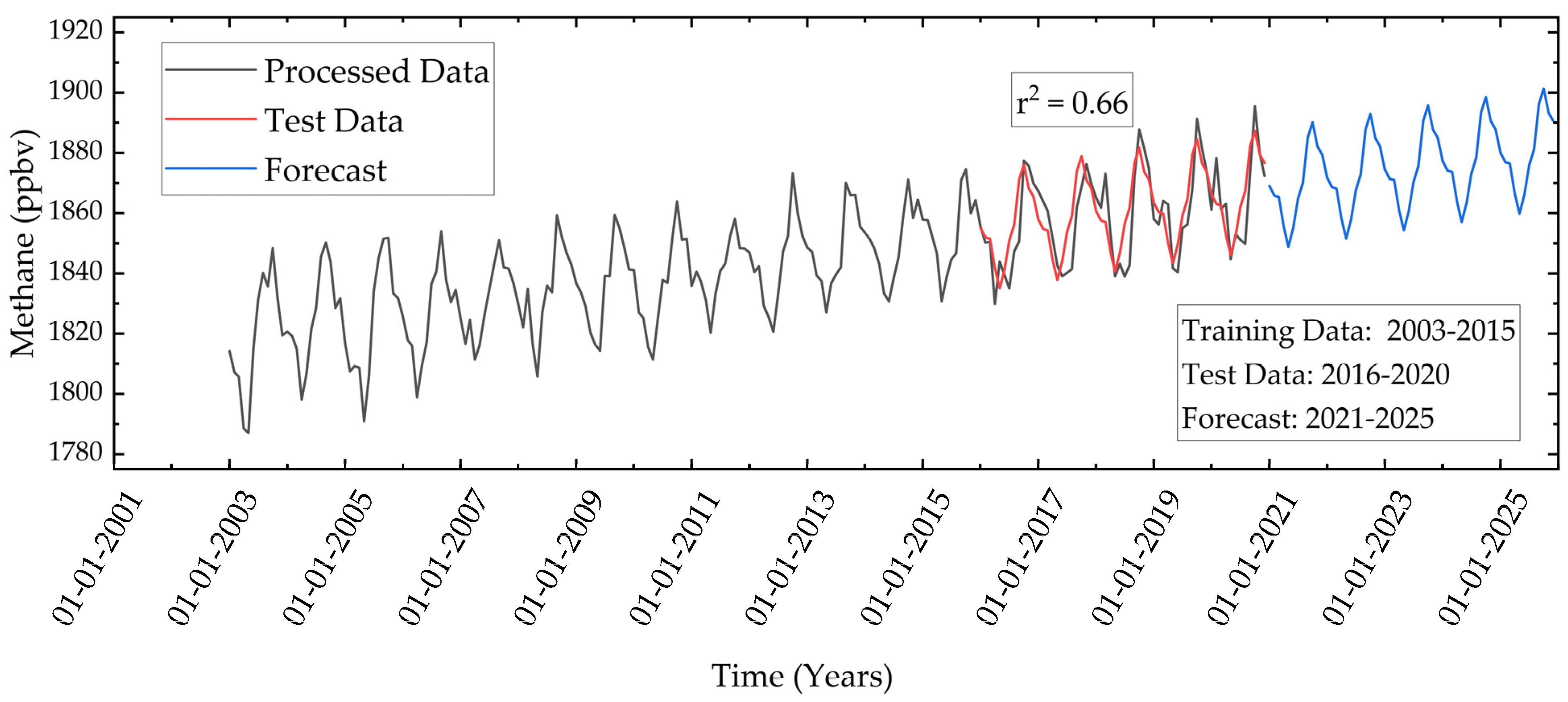
3.3. Time Series Analysis of Pollutants
3.4. Spearman’s Rank Correlation
3.5. Accumulation Index of Soil in Singrauli Region
4. Discussion
Limitations and Recommendation
5. Conclusions
Author Contributions
Funding
Institutional Review Board Statement
Informed Consent Statement
Data Availability Statement
Acknowledgments
Conflicts of Interest
References
- Raghuvanshi, S.P.; Chandra, A.; Raghav, A.K. Carbon dioxide emissions from coal-based power generation in India. Environ. Conver. Manag. 2006, 47, 427–441. [Google Scholar] [CrossRef]
- Wittig, R.; König, K.; Schmidt, M.; Szarzynski, J. A study of climate change and anthropogenic impacts in West Africa. Environ. Sci. Poll. Res. Int. 2007, 14, 182–189. [Google Scholar] [CrossRef] [PubMed]
- Bradshaw, R. Past anthropogenic influence on European forests and some possible genetic consequences. For. Ecol. Manag. 2004, 197, 203–212. [Google Scholar] [CrossRef]
- Prasad, A.; Singh, R. Changes in Himalayan Snow and Glacier Cover Between 1972 and 2000. EOS Trans. AGU 2007, 88, 326. [Google Scholar] [CrossRef]
- Gautam, R.; Hsu, N.C.; Lau, K.M.; Tsay, S.C.; Kafatos, M. Enhanced pre-monsoon warming over the Himalayan-Gangetic region from 1979 to 2007. Geophys. Res. Lett. 2009, 36, L07704. [Google Scholar] [CrossRef]
- Douville, H.; Ribes, A.; Decharme, B.; Alkama, R.; Sheffield, J. Anthropogenic influence on multidecadal changes in reconstructed global evapotranspiration. Nat. Clim. Chang. 2013, 3, 59–62. [Google Scholar] [CrossRef]
- Balakrishnan, K.; Dey, S.; Gupta, T.; Dhaliwal, R.S.; Brauer, M.; Cohen, A.J.; Stanaway, J.D.; Beig, G.; Joshi, T.K.; Aggarwal, A.N. The Impact of Air Pollution on Deaths, Disease Burden, and Life Expectancy across the States of India: The Global Burden of Disease Study 2017. In The Lancet Planetary Health; Elsevier: Amsterdam, The Netherlands, 2019; pp. 26–39. [Google Scholar]
- Sarkodie, S.A.; Owusu, P.A. Impact of meteorological factors on COVID-19 pandemic: Evidence from top 20 countries with confirmed cases. Environ. Res. 2020, 9, 110101. [Google Scholar] [CrossRef]
- Somani, M.; Srivastava, A.N.; Gummadivalli, S.K.; Sharma, A. Indirect implications of COVID-19 towards sustainable environment: An investigation in Indian context. Bioresour. Technol. Rep. 2020, 11, 100491. [Google Scholar] [CrossRef]
- World Health Organization (WHO)/Health Topics/Air Pollution Page. Available online: https://www.who.int/india/health-topics/air-pollution (accessed on 10 May 2022).
- Gaetke, L.M.; Chow, C.K. Copper toxicity, oxidative stress, and antioxidant nutrients. Toxicology 2003, 189, 147–163. [Google Scholar] [CrossRef]
- Turkdogan, M.K.; Fevzi, K.; Kazim, K.; Ilyas, T.; Ismail, U. Heavy metals in soil, vegetables and fruits in the endemic upper gastrointestinal cancer region of Turkey Environ. Toxicol. Pharmacol. 2003, 13, 175–179. [Google Scholar] [CrossRef]
- Liu, X.; Song, Q.; Tang, Y.; Li, W.; Xu, J.; Wu, J.; Wang, F.; Brookes, P.C. Human health risk assessment of heavy metals in soil–vegetable system: A multi-medium analysis. Sci. Total Environ. 2013, 463, 530–540. [Google Scholar] [CrossRef] [PubMed]
- Zhou, H.; Yang, W.; Zhou, X.; Liu, L.; Gu, J.; Wang, W.; Zou, J.; Tian, T.; Peng, P.; Liao, B. Accumulation of heavy metals in vegetable species planted in contaminated soils and the health risk assessment. Int. J. Environ. Res. Public Health 2016, 13, 289. [Google Scholar] [CrossRef]
- Central Electricity Authority, Annual Report 2020–2021. 2021. Available online: https://cea.nic.in/annual-report/?lang=en (accessed on 12 May 2022).
- Venkataraman, C.; Brauer, M.; Tibrewal, K.; Sadavarte, P.; Ma, Q.; Cohen, A.; Chaliyakunnel, S.; Frostad, J.; Klimont, Z.; Martin, R.V.; et al. Source influence on emission pathways and ambient PM2.5 pollution over India (2015–2050). Atmos. Chem. Phys. 2018, 18, 8017–8039. [Google Scholar] [CrossRef] [PubMed]
- IEA. India Energy Outlook 2021, IEA, Paris. 2021. Available online: https://www.iea.org/reports/india-energy-outlook-2021 (accessed on 12 May 2022).
- Bell, F.G.; Bullock, S.E.T.; Halbich, T.F.J.; Lindsay, P. Lindsey: Environment impacts associated with an abandoned mine in the Witbank Coalfield, South Africa. Int. J. Coal. Geol. 2001, 45, 195–216. [Google Scholar] [CrossRef]
- Areendran, G.; Rao, P.; Raj, K.; Mazumdar, S.; Puri, K. Land use/land cover change dynamics analysis in mining areas of Singrauli district in Madhya Pradesh, India. Trop. Ecology. 2013, 54, 239–250. [Google Scholar]
- Bhardwaj, S.; Soni, R.; Gupta, S.K.; Shukla, D.P. Mercury, arsenic, lead and cadmium in waters of the Singrauli coal mining and power plants industrial zone, Central East India. Environ. Monit. Assess. 2020, 192, 251. [Google Scholar] [CrossRef]
- Prasad, A.K.; Singh, R.P.; Kafatos, M. Influence of coal-based thermal power plants on aerosol optical properties in the Indo-Gangetic basin. Geophys. Res. Lett. 2006, 33, 5. [Google Scholar] [CrossRef]
- Singh, R.P.; Kumar, S.; Singh, A.K. Elevated Black Carbon Concentrations and Atmospheric Pollution around Singrauli Coal-Fired Thermal Power Plants (India) Using Ground and Satellite Data. Int. J. Environ. Res. Public Health 2018, 15, 2472. [Google Scholar] [CrossRef]
- Arif, M.; Kumar, R.; Kumar, R.; Zusman, E.; Singh, R.P.; Gupta, A. Assessment of indoor & outdoor black carbon emissions in rural areas of Indo-Gangetic Plain: Seasonal characteristics, source apportionment and radiative forcing. Atmos. Environ. 2018, 191, 227–240. [Google Scholar]
- Singh, R.P.; Chauhan, A. Chapter 1—Sources of atmospheric pollution in India. In Asian Atmospheric Pollution; Elsevier: Amsterdam, The Netherlands, 2021; pp. 1–37. [Google Scholar]
- Dubey, C.S.; Usham, A.L.; Mishra, B.K.; Shukla, D.P.; Singh, P.K.; Singh, A.K. Anthropogenic arsenic menace in contaminated water near thermal power plants and coal mining area of India. Environ. Geochem. Health 2022, 44, 1099–1127. [Google Scholar] [CrossRef]
- Guttikunda, S.K.; Jawahar, P. Atmospheric emissions and pollution from the coal-fired thermal power plants in India. Atmos. Environ. 2014, 92, 449–460. [Google Scholar] [CrossRef]
- Saikawa, E.; Kim, H.; Zhong, M.; Avramov, A.; Zhao, Y.; Janssens-Maenhout, G.; Kurokawa, J.-I.; Klimont, Z.; Wagner, F.; Naik, V. Comparison of emissions inventories of anthropogenic air pollutants and greenhouse gases in China. Atmos. Chem. Phys. 2017, 10, 6393–6421. [Google Scholar] [CrossRef] [Green Version]
- Duncan, B.N.; Lok, N.L.; Thompson, A.M.; Yoshida, Y.; Lu, Z.; Streets, D.G.; Hurwitz, M.M.; Pickering, K.E. A space-based, high-resolution view of notable changes in urban NOx pollution around the world (2005–2014). J. Geophys. Res. Atmos. 2016, 121, 976–996. [Google Scholar] [CrossRef]
- Mandal, A.; Sengupta, D. Radionuclide and trace element contamination around Kolaghat thermal power plant, West Bengal. Curr. Sci. 2005, 88, 617–624. [Google Scholar]
- Mandal, A.; Sengupta, D. An assessment of soil contamination due to heavy metals around a coal fired thermal power plant in India. Environ. Geol. 2006, 51, 409–420. [Google Scholar] [CrossRef]
- Keegan, T.J.; Farago, M.E.; Thornton, I.; Hong, B.; Colvile, R.N.; Pesh, B.; Jakubis, P.; Nieuwenhuijsen, M.J. Dispersion of As and selected heavy metals around a coal burning power station in central Slovakia. Sci. Total Environ. 2006, 358, 61–71. [Google Scholar] [CrossRef]
- Sonwane, D.V.; Lawande, S.P.; Gaikwad, V.B.; Kamble, P.N.; Kuchekar, S.R. Studies on Ground Water Quality Around Kurkumbh Industrial Area, Daund, Pune District. Rayasan J. Chem. 2009, 12, 421–423. [Google Scholar]
- Dwivedi, A.K.; Vankar, P.S. Source identification study of heavy metal contamination in the industrial hub of Unnao, India. Environ. Monit. Assess. 2014, 186, 3531–3539. [Google Scholar] [CrossRef]
- Das, A.; Patel, S.S.; Kumar, R.; Krishna, K.V.S.S.; Dutta, S.; Saha, M.C.; Sengupta, S.; Guha, D. Geochemical sources of metal contamination in a coal mining area in Chhattisgarh, India using lead isotopic ratios. Chemosphere 2018, 197, 152–164. [Google Scholar] [CrossRef]
- Agrawal, P.; Mittal, A.; Prakash, R.; Kumar, M.; Singh, T.B.; Tripathi, S.L. Assessment of Contamination of Soil due to Heavy Metals around Coal Fired Thermal Power Plants at Singrauli Region of India. Bull Environ. Contam. Toxicol. 2010, 85, 219–223. [Google Scholar] [CrossRef]
- Usham, A.L.; Dubey, C.S.; Shukla, D.P.; Mishra, B.K.; Bhartiya, G.P. Sources of fluoride contamination in Singrauli with special reference to Rihand reservoir and its surrounding. J. Geol. Soc. India 2018, 91, 441–448. [Google Scholar] [CrossRef]
- Romana, H.K.; Singh, R.P.; Shukla, D.P. Long Term Air Quality Analysis in Reference to Thermal Power Plants Using Satellite Data in Singrauli Region, India. Int. Arch. Photogramm. Remote Sens. Spat. Inf. Sci. 2020, 43, 829–834. [Google Scholar] [CrossRef]
- Yadav, A.K.; Shirin, S.; Emmanouil, C.; Jamal, A. Effect of seasonal and meteorological variability of air pollution in Singrauli coalfield. Aerosol. Sci. Eng. 2022, 6, 61–70. [Google Scholar] [CrossRef]
- Central Pollution Control Board (CPCB)/CPCB’s Activities/Air Quality Management/National Air Monitoring Programme/Monitoring Network Page. Available online: https://cpcb.nic.in/monitoring-network-3/ (accessed on 10 May 2022).
- Tiwari, M.; Pratap, D.; Kumar, V.; Shukla, N.K. Seasonal variation of Ozone in Industrial area of Singrauli, India. Middle East J. Sci. Res. 2016, 24, 11–14. [Google Scholar]
- Engel-Cox, J.A.; Holloman, C.H.; Coutant, B.W.; Hoff, R.M. Qualitative and quantitative evaluation of MODIS satellite sensor data for regional and urban scale air quality. Atm. Environ. 2004, 38, 2495–2509. [Google Scholar] [CrossRef]
- Lee, H.J.; Coull, B.A.; Bell, M.L.; Koutrakis, P. Use of satellite-based aerosols optical depth and spatial clustering to predict ambient PM2.5 concentrations. Environ. Res. 2012, 118, 8–15. [Google Scholar] [CrossRef]
- Lu, Z.; Streets, D.G.; Foy, B.D.; Krotkov, N.A. Ozone Monitoring Instrument Observations of Interannual Increases in SO2 Emissions from Indian Coal-Fired Power Plants during 2005−2012. Environ. Sci. Technol. 2013, 47, 13993–14000. [Google Scholar] [CrossRef]
- Yadav, A.K.; Hopke, P.K. Characterization of radionuclide activity concentrations and lifetime cancer risk due to particulate matter in the Singrauli Coalfield, India. Environ. Monit. Assess 2020, 192, 680. [Google Scholar] [CrossRef]
- Misra, K.C. Ecno-eco development of Singrauli Coalfields area. In Proceedings of the National Seminar on Eco-Development of Singrauli Area, Japan, Tokyo, 22–23 November 1987. [Google Scholar]
- Majumder, S.; Sarkar, K. Imapct of Mining and Related Activities on Physical and Cultural Environment of Singrauli Coalfield- A Case Study through Application of Remote Sensing Techniques. J. Indian Soc. Remote Sens. 1994, 12, 45–56. [Google Scholar] [CrossRef]
- Bose, R.K.; Leitmann, J. Environmental Profile of the Singrauli Region, India. J. Elsevier. 1996, 13, 71–77. [Google Scholar] [CrossRef]
- EDF. Environment Study of the Singrauli Area: Main Report EDF/NTPC; EDF: New Delhi, India, 1991. [Google Scholar]
- EDF. Environment Study of the Singrauli Area: Aquatic Ecology Edf/NTPC; EDF: New Delhi, India, 1991. [Google Scholar]
- Can, L.; Krotkov, N.K.; Leonard, P. OMI/Aura Sulfur Dioxide (SO2) Total Column L3 1 Day Best Pixel in 0.25 Degree x 0.25 degree V3; Goddard Earth Sciences Data and Information Services Center (GES DISC): Greenbelt, MD, USA, 2021.
- Krotkov, N.A.; Lamsal, L.N.; Marchenko, S.V.; Celarier, E.A.; Bucsela, E.J.; Swartz, W.H. Joanna Joiner and the OMI Core Team, 2019. OMI/Aura NO2 Cloud-Screened Total and Tropospheric Column L3 Global Gridded 0.25 Degree x 0.25 Degree V3; NASA Goddard Space Flight Center, Goddard Earth Sciences Data and Information Services Center (GES DISC): Greenbelt, MD, USA, 2021.
- AIRS Science Team/Joao Teixeira. AIRS/Aqua L3 Monthly CO2 in the Free Troposphere (AIRS-only) 2.5 Degrees x 2 Degrees V005; Goddard Earth Sciences Data and Information Services Center (GES DISC): Greenbelt, MD, USA, 2008.
- AIRS Science Team/Joao Teixeira. AIRS/Aqua L3 Daily Standard Physical Retrieval (AIRS-only) 1 Degree x 1 Degree V006; Goddard Earth Sciences Data and Information Services Center (GES DISC): Greenbelt, MD, USA, 2013.
- Vinutha, H.P.; Poornima, B.; Sagar, B.M. Detection of outliers using interquartile range technique from intrusion dataset. In Information and Decision Sciences; Springer: Singapore, 2018; pp. 511–518. [Google Scholar]
- Time Series. In The Concise Encyclopedia of Statistics; Springer: New York, NY, USA, 2008. [CrossRef]
- Gauthier, T.D. Detecting trends using Spearman’s rank correlation coefficient. Environ. Forensics 2001, 2, 359–362. [Google Scholar] [CrossRef]
- Müller, G. Schwermetalle in den Sedimenten des Rheins-Veränderungen seit 1971. Umschau 1979, 24, 778–783. [Google Scholar]
- Pruteanu, C.G.; Ackland, G.J.; Poon, W.C.K.; Loveday, J.S. When immiscible becomesmiscible-Methane in water at high pressures. Sci. Adv. 2017, 3, e1700240. [Google Scholar] [CrossRef]
- Richter, A.; Wittrock, F.; Burrows, J.P. SO2 measurements with SCIAMACHY. In European Space Agency; ESA SP: Bremen, Germany, 2006. [Google Scholar]
- Kaur, S.; Purohit, M.K. Rainfall Statistics of India-2012; Report No. ESSO/IMD/HS/R.F.REP/02(2013)/16; Indian Meteorological Department (IMD): New Delhi, India, 2013.
- Chauhan, A.; Kumar, R.; Singh, R.P. Coupling between Land-Ocean-Atmosphere and Pronounced Changes in Atmospheric/Meteorological Parameters Associated with the Hudhud Cyclone of October 2014. Int. J. Environ. Res. Public Health. 2018, 15, 2759. [Google Scholar] [CrossRef] [PubMed]
- Sven, N.; Naeem, M.F.; Tans, P. Estimating the short-time rate of change in the trend of the Keeling curve. Sci. Rep. 2020, 10, 21222. [Google Scholar]
- Menz, F.C.; Seip, H.M. Acid rain in Europe and the United States: An update. Environ. Sci. Policy 2004, 7, 253–265. [Google Scholar] [CrossRef]
- Rogalski, L.; Smoczynski, L.; Sławomir, K.; Leszek, L.; Ewa, M. Changes in sulphur dioxide concentrations in the atmospheric air assessed during short-term measurements in the vicinity of Olsztyn, Poland. J. Elem. 2014, 19, 735–748. [Google Scholar]
- Misra, P.; Takigawa, M.; Khatri, P.; Dhaka, S.K.; Dimri, A.P.; Yamaji, K.; Kajino, M.; Takeuchi, W.; Imasu, R.; Nitta, K. Nitrogen oxides concentration and emission change detection during COVID-19 restrictions in North India. Sci. Rep. 2021, 11, 9800. [Google Scholar] [CrossRef]
- Van, D.R.; Crippa, M.; Anssens-Maenhout, G.; Guizzardi, D.; Dentener, F. Global Trends of Methane Emissions and Their Impacts on Ozone Concentrations; EUR 29394 EN; Publications Office of the European Union: Luxembourg, 2018. [Google Scholar] [CrossRef]
- Wang, H.; Ding, J.; Xu, J.; Wen, J.; Han, J.; Wang, K.; Shi, G.; Feng, Y.; Ivey, C.E.; Wang, Y.; et al. Aerosols in an arid environment: The role of aerosol water content, particulate acidity, precursors, and relative humidity on secondary inorganic aerosols. Sci. Total Environ. 2019, 646, 564–572. [Google Scholar] [CrossRef]
- Olivier, J.G.; Greet, J.G.; Marilena, M.M.; Peters, J.A.H.W. Trends in Global CO2 Emissions: 2016 Report; PBL Netherlands Environmental Assessment Agency: The Hague, The Netherlands, 2017. [Google Scholar]
- Turekian, K.K.; Wedepohl, K.H. Distribution of the elements in some major units of the earth’s crust. Geol. Soc. Am. Bulletin. 1961, 72, 175–192. [Google Scholar] [CrossRef]
- Kumari, M.; Sarma, K.; Sharma, R. Using Moran’s I and GIS to study the spatial pattern of land surface temperature in relation to land use/cover around a thermal power plant in Singrauli district, Madhya Pradesh, India. Remote Sens. Appl. Soc. Environ. 2019, 15, 100239. [Google Scholar] [CrossRef]
- Lu, Z.; Streets, D.G. Increase in NOx emissions from Indian thermal power plants during 1996–2010: Unit-based inventories and multisatellite observations. Environ. Sci. Techol. 2013, 46, 7463–7470. [Google Scholar] [CrossRef] [PubMed]
- Mittal, M.L.; Sharma, C.; Singh, R. Decadal emission estimates of carbon dioxide, sulfur dioxide and nitric oxide emissions from coal burning in electric power generation plants in India. Environ. Monit. Assess 2014, 186, 6857–6866. [Google Scholar] [CrossRef]
- Lazo, J.; Gerson, A.; Watts, D. An impact study of COVID-19 on the electricity sector: A comprehensive literature review and Ibero-American survey. Renew. Sustain. Energy Rev. 2022, 1, 112135. [Google Scholar] [CrossRef]
- Kumari, P.; Toshniwal, D. Impact of lockdown on air quality over major cities across the globe during COVID-19 pandemic. Urban Clim. 2020, 34, 100719. [Google Scholar] [CrossRef]
- Guttikunda, S.K.; Jawahar, P. Evaluation of particulate pollution and health impacts from planned expansion of coal-fired thermal power plants in India using WRF-CAMx modeling system. Aerosol. Air Qual. Res. 2018, 18, 3187–3202. [Google Scholar] [CrossRef]


| S. No. | Name of TPP | Location | Installation/Expansion Month | Capacity (MW) |
|---|---|---|---|---|
| 1 | NTPC | Rihand | January,2005 | 500 |
| 2 | NTPC | Rihand | September, 2005 | 500 |
| 3 | NTPC | Vindhyachal | July, 2006 | 500 |
| 4 | NTPC | Vindhyachal | March, 2007 | 500 |
| 5 | Lanco | Anpara | December, 2011 | 600 |
| 6 | Lanco | Anpara | January, 2012 | 600 |
| 7 | NTPC | Rihand | May, 2012 | 500 |
| 8 | NTPC | Vindhyachal | June, 2012 | 500 |
| 9 | NTPC | Vindhyachal | March, 2013 | 500 |
| 10 | Essar | Sasan | December, 2012 | 600 |
| 11 | Reliance | Sasan | March, 2013 | 660 |
| 12 | Reliance | Sasan | December, 2013 | 660 |
| 13 | Jaypee | Nigre | December, 2013 | 660 |
| 14 | Reliance | Sasan | March, 2014 | 660 |
| 15 | Jaypee | Nigre | March, 2014 | 660 |
| 16 | Reliance | Sasan | May, 2014 | 660 |
| 17 | Reliance | Sasan | August, 2014 | 660 |
| 18 | Reliance | Sasan | March, 2015 | 660 |
| 19 | Hindalco | Baragawon | July, 2015 | 900 |
| 20 | NTPC | Vindhyachal | August, 2015 | 500 |
| 21 | UPRVUNL | Anpara | May, 2016 | 500 |
| 22 | UPRVUNL | Anpara | October, 2016 | 500 |
| 23 | Essar | Sasan | May, 2017 | 600 |
| S. No. | Pollutant | Unit | Sensor | Data Time | Spatial Resolution |
|---|---|---|---|---|---|
| 1 | SO2 | DU | OMI | 2005–2020 | 0.25 × 0.25° |
| 2 | NO2 | ppm | OMI | 2005–2020 | 0.25 × 0.25° |
| 3 | CO2 | ppm | AIRS | 2003–2016 | 2 × 2.5° |
| 4 | CH4 | ppbv | AIRS | 2003–2020 | 1 × 1° |
| S.No. | Sampling Site | Latitude | Longitude | As | F | Ti | Fe | Cr | Pb | Cu | Zn | Mn |
|---|---|---|---|---|---|---|---|---|---|---|---|---|
| Acceptable Limit (WHO, 1996) | 2 mg/kg | 48 mg/kg | 300 mg/kg | 48 mg/kg | 42 mg/kg | 2 mg/kg | 30 mg/kg | 60 mg/kg | 450 mg/kg | |||
| 1 | Kakri Coal Mines | 24°10′25″ | 82°45′32″ | 1.5 | 3.6 | 1540.5 | 9502.9 | 29.0 | 12.5 | 10.3 | 46.4 | 253.8 |
| 2 | Near Bina Coal Mines | 24°9′55″ | 82°44′46″ | 1.0 | 4.87 | 739.1 | 11,518.9 | 23.4 | 14.6 | 4.1 | 49.2 | 142.8 |
| 3 | Bina Coal Mines | 24°9′25″ | 82°4′40″ | 2.0 | 5.32 | 2254.7 | 8251.5 | 141.2 | 35.1 | 37.1 | 119.2 | 632.9 |
| 4 | Rihand Dam | 24°12′30″ | 83°00′05″ | 2.5 | 2.84 | 2794.3 | 22,424.7 | 65.0 | 5.1 | 12.2 | 31.8 | 1187.8 |
| 5 | NTPC Shaktinagar TPP | 24°5′55″ | 82°42′33″ | 1.3 | 6.1 | 6276.8 | 11,965.0 | 89.1 | 3.4 | 40.2 | 67.5 | 380.5 |
| 6 | Vindhayachal TPP | 24°5′18″ | 82°40′55″ | 2.6 | 3.9 | 2275.0 | 20,126.1 | 94.8 | 31.8 | 14.2 | 120.1 | 485.2 |
| 7 | Lanco TPP | 24°12′22″ | 82°48′44″ | 1.0 | 1.4 | 2553.3 | 43,610.6 | 211.1 | 7.0 | 3.3 | 79.4 | 585.9 |
| 8 | Anpara TPP | 24°11′27″ | 82°47′51″ | 0.9 | 0.83 | 6878.2 | 43,129.7 | 93.3 | 13.1 | 29.6 | 492.2 | 701.3 |
| 9 | Hindalco Industries | 24°13′05″ | 83°02′06″ | 1.3 | 2.03 | 3774.6 | 44,302.1 | 107.2 | 70.1 | 16.4 | 108.7 | 735.8 |
| 10 | Obra TPP | 24°26′36″ | 82°59′05″ | 4.1 | 3.8 | 2031.3 | 30,121.4 | 95.8 | 70.4 | 17.3 | 70.9 | 521.3 |
| 11 | Near Vindhayanagar | 24°04′53″ | 82°39′15″ | 2.1 | 0.33 | 2478.6 | 15,511.9 | 33.0 | 17.6 | 7.9 | 39.5 | 354.7 |
| 12 | Between Bina and Kakri | 24°09′37″ | 82°45′39″ | 1.8 | 5.81 | 1510.5 | 13,463.3 | 25.3 | 11.8 | 10.2 | 30.8 | 286 |
| 13 | Bina Coal Mines | 24°09′6.8″ | 82°46′01″ | 3.6 | 16.9 | 2322.0 | 28,976.0 | 99.3 | 84.6 | 24.2 | 64.4 | 558.2 |
| 14 | Khadia Coal Mines | 24°06′54″ | 82°43′26″ | 3.5 | 28.5 | 1737.6 | 29,921.4 | 93.9 | 80.9 | 23.7 | 65.3 | 484.2 |
| 15 | Renusagar TPP | 24°10′37″ | 82°47′26″ | 2.6 | 43.5 | 1871.5 | 15,249.8 | 30.4 | 9.7 | 4.9 | 83.9 | 359.9 |
| 16 | Singrauli Reservoir | 24°07′58″ | 82°48′02″ | 1.5 | 37.8 | 522.4 | 7261.3 | 13.7 | 7.5 | 2.0 | 32.1 | 221.3 |
| Class | Values of Igeo | Soil Quality |
|---|---|---|
| 0 | I ≤ 0 | unpolluted |
| 1 | 0–1 | unpolluted to moderately polluted |
| 2 | 1–2 | moderately polluted |
| 3 | 2–3 | moderately to highly polluted |
| 4 | 3–4 | highly polluted |
| 5 | 4–5 | highly to extremely high polluted |
| 6 | I ≥ 5 | extremely high polluted |
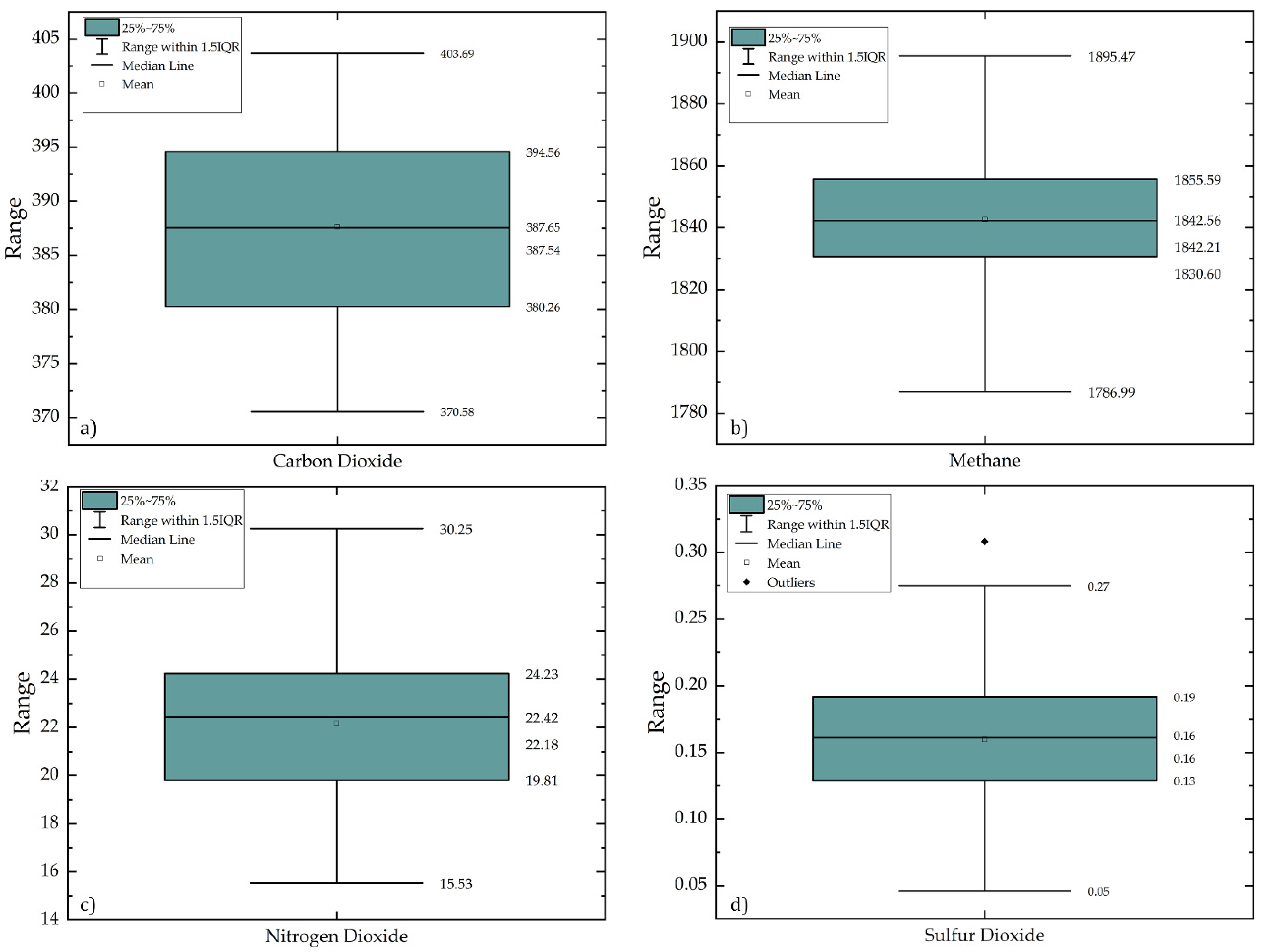
| S.NO | Parameter | Acceptable Limit | Minimum | Maximum | Average | Standard Deviation | Variance |
|---|---|---|---|---|---|---|---|
| 1 | Carbon dioxide (ppm) | 400 ppm | 370.58 | 403.69 | 387.65 | ±8.70 | 75.52 |
| 2 | Methane (ppbv) | 1786.99 | 1895.47 | 1842.56 | ±20.18 | 407.14 | |
| 3 | Nitrogen dioxide (ppm) | 0.053 ppm | 15.53 | 30.25 | 22.18 | ±3.15 | 9.92 |
| 4 | Sulfur dioxide (DU) | 0.10 DU | 0.05 | 0.27 | 0.16 | ±0.05 | 0.002 |
| AOD | SO2 | NO2 | Methane | PM2.5 | PM10 | CO2 | |
|---|---|---|---|---|---|---|---|
| AOD | 1.00 | 0.76 | 0.86 | 0.45 | 0.44 | 0.96 | 0.03 |
| SO2 | 0.09 | 1.00 | 0.76 | 0.03 | 0.19 | 0.22 | 0.00 |
| NO2 | 0.55 | 0.09 | 1.00 | 0.76 | 0.03 | 0.01 | 0.00 |
| CH4 | −0.23 | 0.59 | 0.09 | 1.00 | 0.15 | 0.10 | 0.00 |
| PM2.5 | −0.24 | 0.39 | 0.60 | 0.42 | 1.00 | 0.00 | NA |
| PM10 | 0.02 | 0.36 | 0.67 | 0.48 | 0.82 | 1.00 | NA |
| CO2 | 0.20 | 0.28 | 0.47 | 0.48 | NA | NA | 1.00 |
| Location | As | Ti | Fe | Cr | Pb | Zn | Cu | Mn | Cumulative Index |
|---|---|---|---|---|---|---|---|---|---|
| Kakri Coal Mines | 1 | 0 | 0 | 0 | 1 | 1 | 1 | 0 | 4 |
| Near Bina Coal Mines | 0 | 0 | 0 | 0 | 1 | 2 | 0 | 0 | 3 |
| Bina Coal Mines | 1 | 1 | 0 | 2 | 2 | 3 | 3 | 0 | 12 |
| Rihand Dam | 1 | 0 | 1 | 4 | 0 | 0 | 1 | 0 | 7 |
| NTPC Shaktinagar TPP | 0 | 2 | 0 | 1 | 0 | 2 | 3 | 0 | 8 |
| Vindhayachal TPP | 1 | 1 | 1 | 1 | 2 | 3 | 2 | 0 | 11 |
| Lanco TPP | 0 | 1 | 2 | 3 | 0 | 2 | 0 | 0 | 8 |
| Anpara TPP | 0 | 2 | 2 | 1 | 1 | 5 | 3 | 1 | 15 |
| Hindalco Industries | 0 | 0 | 2 | 5 | 2 | 1 | 2 | 1 | 13 |
| Obra TPP | 2 | 0 | 2 | 3 | 3 | 2 | 2 | 0 | 14 |
| Near Vindhayanagar | 1 | 1 | 1 | 1 | 1 | 1 | 1 | 0 | 7 |
| Between Bina and Kakri | 1 | 0 | 0 | 0 | 1 | 1 | 1 | 0 | 4 |
| Bina Coal Mines | 2 | 1 | 1 | 1 | 4 | 2 | 3 | 0 | 14 |
| Khadia Coal Mines | 2 | 0 | 2 | 1 | 3 | 2 | 2 | 0 | 12 |
| Renusagar TPP | 1 | 0 | 1 | 0 | 0 | 2 | 0 | 0 | 4 |
| Singrauli Reservoir | 0 | 0 | 0 | 0 | 0 | 1 | 0 | 0 | 1 |
Publisher’s Note: MDPI stays neutral with regard to jurisdictional claims in published maps and institutional affiliations. |
© 2022 by the authors. Licensee MDPI, Basel, Switzerland. This article is an open access article distributed under the terms and conditions of the Creative Commons Attribution (CC BY) license (https://creativecommons.org/licenses/by/4.0/).
Share and Cite
Romana, H.K.; Singh, R.P.; Dubey, C.S.; Shukla, D.P. Analysis of Air and Soil Quality around Thermal Power Plants and Coal Mines of Singrauli Region, India. Int. J. Environ. Res. Public Health 2022, 19, 11560. https://doi.org/10.3390/ijerph191811560
Romana HK, Singh RP, Dubey CS, Shukla DP. Analysis of Air and Soil Quality around Thermal Power Plants and Coal Mines of Singrauli Region, India. International Journal of Environmental Research and Public Health. 2022; 19(18):11560. https://doi.org/10.3390/ijerph191811560
Chicago/Turabian StyleRomana, Harsimranjit Kaur, Ramesh P. Singh, Chandra S. Dubey, and Dericks P. Shukla. 2022. "Analysis of Air and Soil Quality around Thermal Power Plants and Coal Mines of Singrauli Region, India" International Journal of Environmental Research and Public Health 19, no. 18: 11560. https://doi.org/10.3390/ijerph191811560
APA StyleRomana, H. K., Singh, R. P., Dubey, C. S., & Shukla, D. P. (2022). Analysis of Air and Soil Quality around Thermal Power Plants and Coal Mines of Singrauli Region, India. International Journal of Environmental Research and Public Health, 19(18), 11560. https://doi.org/10.3390/ijerph191811560