
Air Quality Assessment by the Determination of Trace Elements in Lichens (Xanthoria calcicola) in an Industrial Area (Sicily, Italy)


Abstract
:1. Introduction
2. Materials and Methods
2.1. Description of the Study Area
2.2. Sampling and Analytical Method
2.3. Statistical Analysis and Spatial Distribution
2.4. Geochemical Indices for Evaluating Trace Element Pollution
- CF 0–1 No contamination
- CF > 1–2 Suspected contamination
- CF > 2–3.5 Slight contamination
- CF > 3.5–8 Moderate contamination
- CF > 8–27 Severe contamination
- CF > 27 Extreme contamination
- ERI < 5 Low risk
- 5 ≤ ERI < 10 Moderate risk
- 10 ≤ ERI < 20 Considerable risk
- 20 ≤ ERI < 40 High risk
- ERI ≥ 40 Very high risk
3. Results and Discussion
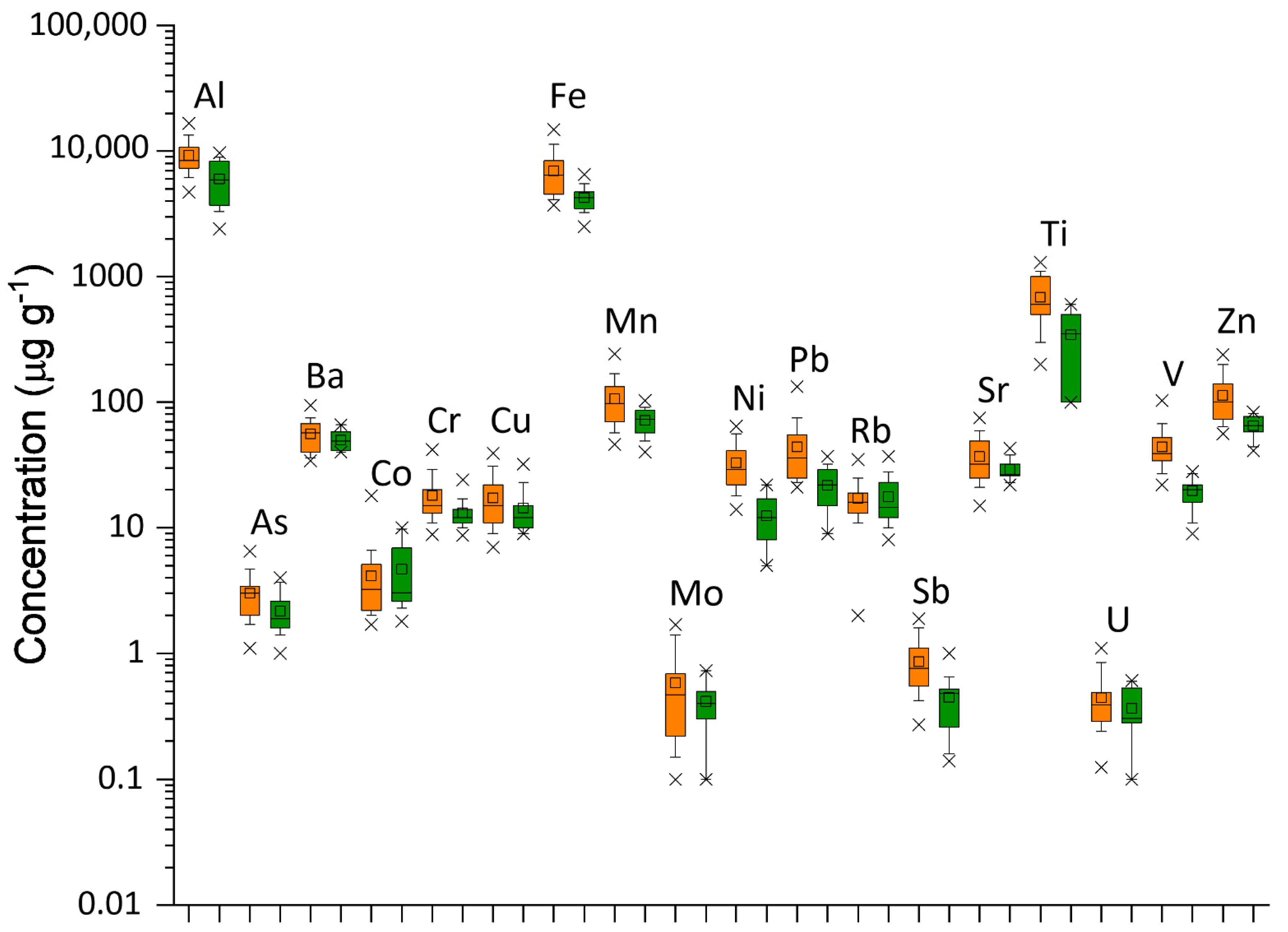
3.1. Descriptive Statistics
3.2. Enrichment Factor and Geochemical Indices
3.3. Pollution Assessment
4. Conclusions
Author Contributions
Funding
Institutional Review Board Statement
Informed Consent Statement
Data Availability Statement
Conflicts of Interest
References
- Moreno, T.; Querol, X.; Alastuey, A.; Reche, C.; Cusack, M.; Amato, F.; Pandolfi, M.; Pey, J.; Richard, A.; Prévôt, A.S.H.; et al. Variations in time and space of trace metal aerosol concentrations in urban areas and their surroundings. Atmos. Chem. Phys. 2011, 11, 9415–9430. [Google Scholar] [CrossRef] [Green Version]
- Fernández-Camacho, R.; Rodríguez, S.; de la Rosa, J.; Sánchez de la Campa, A.M.; Alastuey, A.; Querol, X.; González-Castanedo, Y.; Garcia-Orellana, I.; Nava, S. Ultrafine particle and fine trace metal (As, Cd, Cu, Pb and Zn) pollution episodes induced by industrial emissions in Huelva, SW Spain. Atmos. Environ. 2012, 61, 507–517. [Google Scholar] [CrossRef] [Green Version]
- Pan, Y.; Tian, S.; Li, X.; Sun, Y.; Li, Y.; Wentworth, G.R.; Wang, Y. Trace elements in particulate matter from metropolitan regions of Northern China: Sources, concentrations and size distributions. Sci. Total Environ. 2015, 537, 9–22. [Google Scholar] [CrossRef] [PubMed]
- Pan, Y.P.; Wang, Y.S. Atmospheric wet and dry deposition of trace elements at 10 sites in northern China. Atmos. Chem. Phys. 2015, 15, 951–972. [Google Scholar] [CrossRef] [Green Version]
- Koz, B.; Cevik, U.; Akbulut, S. Heavy metal analysis around Murgul (Artvin) copper mining area of Turkey using moss and soil. Ecol. Indic. 2012, 20, 17–23. [Google Scholar] [CrossRef]
- Turkyilmaz, A.; Sevik, H.; Cetin, M.; Ahmaida Saleh, E.A. Changes in heavy metal accumulation depending on traffic density in some landscape plants. Pol. J. Environ. Stud. 2018, 27, 2277–2284. [Google Scholar] [CrossRef]
- Koedrith, P.; Kim, H.; Weon, J.I.; Seo, Y.R. Toxicogenomic approaches for understanding molecular mechanisms of heavy metal mutagenicity and carcinogenicity. Int. J. Hyg. Environ. Health 2013, 216, 587–598. [Google Scholar] [CrossRef]
- Caballero-Segura, B.; Ávila-Pérez, P.; Barrera Díaz, C.E.; Ramírez García, J.J.; Zarazúa, G.; Soria, R.; Ortiz-Oliveros, H.B. Metal content in mosses from the Metropolitan Area of the Toluca Valley: A comparative study between inductively coupled plasma optical emission spectrometry (ICP-OES) and total reflection X-ray fluorescence spectrometry (TXRF). Int. J. Environ. Anal. Chem. 2014, 94, 1288. [Google Scholar] [CrossRef]
- Conti, M.; Cecchetti, G. Biological monitoring: Lichens as bioindicators of air pollution assessment—A review. Environ. Pollut. 2001, 114, 471–492. [Google Scholar] [CrossRef]
- Bing, H.; Wu, Y.; Li, J.; Xiang, Z.; Luo, X.; Zhou, J.; Sun, H.; Zhang, G. Biomonitoring trace element contamination impacted by atmospheric deposition in China’s remote mountains. Atmos. Res. 2019, 224, 30–41. [Google Scholar] [CrossRef]
- Abas, A.; Sulaiman, N.; Adnan, N.R.; Aziz, S.A.; Nawang, W.N.S.W. Using lichen (Dirinaria sp.) as bio-indicator for airborne heavy metal at selected industrial areas in Malaysia. Environ. Asia 2019, 12, 85–90. [Google Scholar]
- Oksanen, J.; Laara, E.; Zobel, K. Statistical analysis of bioindicator value of epiphytic lichens. Lichenologist 1991, 23, 167–180. [Google Scholar] [CrossRef]
- Nimis, P.; Scheidegger, C.; Wolseley, P. Monitoring with Lichens—Monitoring Lichens; Springer: Dordrecht, The Netherlands, 2002. [Google Scholar]
- Spagnuolo, V.; Zampella, M.; Giordano, S.; Adamo, P. Cytological stress and element uptake in moss and lichen exposed in bags in urban area. Ecotoxicol. Environ. Saf. 2011, 74, 1434–1443. [Google Scholar] [CrossRef]
- Malaspina, P.; Giordani, P.; Modenesi, P.; Abelmoschi, M.L.; Magi, E.; Soggia, F. Bioaccumulation capacity of two chemical varieties of the lichen Pseudevernia furfuracea. Ecol. Indic. 2014, 45, 605–610. [Google Scholar] [CrossRef]
- Sujetoviene, G.; Galinyte, V. Effects of the urban environmental conditions on the physiology of lichen and moss. Atmos. Pollut. Res. 2016, 7, 611–618. [Google Scholar] [CrossRef]
- De La Cruz, A.R.H.; De La Cruz, J.K.H.; Tolentino, A.; Gioda, A. Trace element biomonitoring in the Peruvian andes metropolitan region using Flavoparmelia caperata lichen. Chemosphere 2018, 210, 849–858. [Google Scholar] [CrossRef] [PubMed]
- Ndlovu, N.B.; Frontasyeva, M.V.; Newman, R.T.; Maleka, P.P. Active biomonitoring of atmospheric pollution in the Western Cape (South Africa) using INAA and ICP-MS. J. Radioanal. Nucl. Chem. 2019, 322, 1549–1559. [Google Scholar] [CrossRef]
- Ramić, E.; Huremović, J.; Muhić-Šarac, T.; Đug, S.; Žero, S.; Olovčić, A. Biomonitoring of air pollution in bosnia and herzegovina using epiphytic lichen Hypogymnia physodes. Bull. Environ. Contam. Toxicol. 2019, 102, 763–769. [Google Scholar] [CrossRef]
- Rola, K.; Osyczka, P. Temporal changes in accumulation of trace metals in vegetative and generative parts of Xanthoria parietina lichen thalli and their implications for biomonitoring studies. Ecol. Indic. 2019, 96, 293–302. [Google Scholar] [CrossRef]
- Boonpeng, C.; Sriviboon, C.; Polyiam, W.; Sangiamdee, D.; Watthana, S.; Boonpragob, K. Assessing atmospheric pollution in a petrochemical industrial district using a lichen-air quality index (LiAQI). Ecol. Indic. 2018, 95, 589–594. [Google Scholar] [CrossRef]
- Doğrul-Demiray, A.; Yolcubal, I.; Hakan-Akyol, N.; Çobanoğlu, G. Biomonitoring of airborne metals using the Lichen Xanthoria parietina in Kocaeli Province, Turkey. Ecol. Indic. 2012, 18, 632–643. [Google Scholar]
- Loppi, S.; Pirintsos, S.A. Epiphytic lichens as sentinels for heavy metal pollution at forest ecosystems (central Italy). Environ. Poll. 2003, 121, 327–332. [Google Scholar] [CrossRef]
- Bačkor, M.; Loppi, S. Interactions of lichens with heavy metals. Biol. Plant. 2009, 53, 214–222. [Google Scholar]
- Scerbo, R.; Possenti, L.; Lampugnani, L.; Ristori, T.; Barale, R.; Barghigiani, C. Lichen (Xanthoria parietina) biomonitoring of trace element contamination and air quality assessment in Livorno Province (Tuscany, Italy). Sci. Total Environ. 1999, 241, 91–106. [Google Scholar] [CrossRef]
- Policnik, H.; Simoncic, P.; Batic, F. Monitoring air quality with lichens: A comparison between mapping in forest sites and in open areas. Environ. Pollut. 2008, 151, 395–400. [Google Scholar] [CrossRef] [PubMed]
- Gerdol, R.; Marchesini, R.; Iacumin, P.; Brancaleoni, L. Monitoring temporal trends of air pollution in an urban area using mosses and lichens as biomonitors. Chemistry 2014, 108, 388–395. [Google Scholar] [CrossRef]
- Kularatne, K.I.A.; De Freitas, C.R. Epiphytic lichens as biomonitors of airborne heavy metal pollution. Environ. Exp. Bot. 2013, 88, 24–32. [Google Scholar] [CrossRef]
- Bargagli, R.; Mikhailova, I. Accumulation of inorganic contaminants. In Monitoring with Lichens−Monitoring Lichens; NATO Science Series; Nimis, P.L., Scheidegger, C., Wolseley, P.A., Eds.; Springer: Berlin/Heidelberg, Germany, 2002; Volume 7, pp. 65–84. [Google Scholar]
- Paoli, L.; Munzi, S.; Guttová, A.; Senko, D.; Sardella, G.; Loppi, S. Lichens as suitable indicators of the bio- logical effects of atmospheric pollutants around a municipal solid waste incinerator (S Italy). Ecol. Indic. 2015, 52, 362–370. [Google Scholar] [CrossRef]
- Fano, V.; Cernigliaro, A.; Scondotto, S.; Addario, S.P.; Caruso, S.; Mira, A.; Forastiere, F.; Perucci, C.A. Mortality (1995−2000) and hospital admissions (2001–2003) in the industrial area of Gela. Epidemiol. Prev. 2006, 30, 27–32. [Google Scholar]
- Bianchi, F.; Bianca, S.; Barone, C.; Pierini, A. Updating of the prevalence of congenital anomalies among resident births in the Municipality of Gela (Southern Italy). Epidemiol. Prev. 2014, 38, 219–226. [Google Scholar]
- Italian Law 349/1986 Istituzione del Ministero Dell’ambiente e Norme in Materia di Danno Ambientale. (GU n.162 del 15-7-1986—Suppl. Ordinario n. 59). Available online: https://www.normattiva.it/uri-res/N2Ls?urn:nir:stato:legge:1986-07-08;349!vig= (accessed on 1 March 2022).
- Italian Law 426/1998. Nuovi Interventi in Campo Ambientale. (GU n.291 del 14-12-1998). Available online: https://www.normattiva.it/uri-res/N2Ls?urn:nir:stato:legge:1998;426 (accessed on 1 March 2022).
- Carbone, S. Note Illustrative Della Carta Geologica d’Italia Scala 1:50,000, Foglio 641 Augusta Ed. ISPRA—Regione Siciliana, 2011; ISBN 978-88-240-2965-0. [Google Scholar]
- Agenzia Regionale per la Protezione per L’ambiente (ARPA, Sicilia). Rapporto Sulla Qualità Dell’aria nel Comprensorio Dell’area ad Elevato Rischio di Crisi Ambientale di Siracusa. 2018. Available online: http://www.provincia.siracusa.it/rapp_aria_2018.pdf (accessed on 1 March 2022).
- Cressie, N.A.C. Statistics for Spatial Data; John Wiley and Sons, Inc.: New York, NY, USA, 1991; p. 900. [Google Scholar]
- Rutkowski, P.; Diatta, J.; Konatowska, M.; Andrzejewska, A.; Tyburski, Ł.; Przybylski, P. Geochemical referencing of natural forest contamination in Poland. Forests 2020, 11, 157. [Google Scholar] [CrossRef] [Green Version]
- Fernández, J.A.; Carballeira, A.A. comparison of indigenous mosses and topsoils for use in monitoring atmospheric heavy metal deposition in Galicia (northwest Spain). Environ. Pollut. 2001, 114, 431–441. [Google Scholar] [CrossRef]
- Shakya, K.; Chettri, M.K.; Sawidis, T. Use of mosses for the survey of heavy metal deposition in ambient air of the Kathmandu valley applying active monitoring technique. Ecoprint 2012, 19, 17–29. [Google Scholar] [CrossRef] [Green Version]
- Salo, H.; Bućko, M.S.; Vaahtovuo, E.; Limo, J.; Mäkinen, J.; Pesonen, L.J. Biomonitoring of air pollution in SW Finland by magnetic and chemical measurements of moss bags and lichens. J. Geochem. Explor. 2012, 115, 69–81. [Google Scholar] [CrossRef]
- Hakanson, L. An ecological risk index for aquatic pollution control. A sedimentological approach. Water Res. 1980, 14, 975–1001. [Google Scholar] [CrossRef]
- Qing, X.; Yutong, Z.; Shenggao, L. Assessment of heavy metal pollution and human health risk in urban soils of steel industrial city (Anshan), Liaoning, Northeast China. Ecotoxicol. Environ. Saf. 2015, 120, 377–385. [Google Scholar] [CrossRef]
- Wu, S.; Peng, S.; Zhang, X.; Wu, D.; Luo, W.; Zhang, T.; Zhou, S.; Yang, G.; Wan, H.; Wu, L. Levels and health risk assessments of heavy metals in urban soils in Dongguan, China. J. Geochem. Explor. 2015, 148, 71–78. [Google Scholar] [CrossRef]
- Liu, C.; Zhou, P.; Fang, Y. Monitoring Airborne Heavy Metal Using Mosses in the City of Xuzhou, China. Bull. Environ. Contam. Toxicol. 2016, 96, 638–644. [Google Scholar] [CrossRef]
- Hussain, S.; Hoque, R.R. Biomonitoring of metallic air pollutants in unique habitations of the Brahmaputra Valley using moss species—Atrichum angustatum: Spatiotemporal deposition patterns and sources. Environ. Sci. Pollut. Res. 2022, 29, 10617–10634. [Google Scholar] [CrossRef]
- Bargagli, R. Trace Elements in Terrestrial Plants. An Ecophysiological Approach to Biomonitoring and Biorecovery; Springer: Berlin/Heidelberg, Germany, 1998; p. 324. [Google Scholar]
- Hsu, C.Y.; Chiang, H.C.; Lin, S.L.; Chen, M.J.; Lin, T.Y.; Chen, Y.C. Elemental characterization and source apportionment of PM10 and PM2.5 in the western coastal area of central Taiwan. Sci. Total Environ. 2016, 541, 1139–1150. [Google Scholar] [CrossRef]
- Brunialti, G.; Frati, L. Biomonitoring of nine elements by the lichen Xanthoria parietina in Adriatic Italy: A retrospective study over a 7-year time span. Sci. Total Environ. 2007, 387, 289–300. [Google Scholar] [CrossRef] [PubMed]
- Kaiser, H.F. The varimax criteria for analytical rotation in factor analysis. Psychometrika 1958, 23, 187–200. [Google Scholar] [CrossRef]
- Hernandez, L.; Probst, A.; Probst, J.L.; Ulrich, E. Heavy metal distribution in some French forest soils: Evidence for atmospheric contamination. Sci. Total Environ. 2003, 312, 195–219. [Google Scholar] [CrossRef] [Green Version]
- ATSDR. Toxicological Profile for Vanadium. U.S. Department of Health and Human Services. Public Health Service; Agency for Toxic Substances and Disease Registry: Atlanta, GA, USA, 2012. [Google Scholar]
- Mehri, A. Trace Elements in Human Nutrition (II)—An Update. Int. J. Prev. Med. 2020, 11, 2. [Google Scholar] [CrossRef] [PubMed]
- Duce, R.A.; Hoffman, G.L. Atmospheric vanadium transport to the ocean. Atmos. Environ. 1976, 10, 989–996. [Google Scholar] [CrossRef]
- Bosco, M.L.; Dongarrà, G.; Varrica, D. Case study: Inorganic pollutants associated with particulate matter from an area near a petrochemical plant. Environ. Res. 2005, 99, 18–30. [Google Scholar] [CrossRef]
- Genchi, G.; Carocci, A.; Lauria, G.; Sinicropi, M.S.; Catalano, A. Nickel: Human Health and Environmental Toxicology. Int. J. Environ. Res. Public Health 2020, 17, 679. [Google Scholar] [CrossRef] [Green Version]
- Zhao, J.; Shi, X.; Castranova, V.; Ding, M. Occupational toxicology of nickel and nickel compounds. J. Environ. Pathol. Toxicol. Oncol. 2009, 28, 177–208. [Google Scholar] [CrossRef]
- Zambelli, B.; Ciurli, S. Nickel and human health. Met. Ions Life Sci. 2013, 13, 321–357. [Google Scholar]
- McGregor, D.B.; Baan, R.A.; Partensky, C.; Rice, J.M.; Wilbourn, J.D. Evaluation of the carcinogenic risks to humans associated with surgical implants and other foreign bodies—A report of an IARC Monographs Programme Meeting. International Agency for Research on Cancer. Eur. J. Cancer 2000, 36, 307–313. [Google Scholar] [CrossRef]
- Zambelli, B.; Uversky, V.N.; Ciurli, S. Nickel impact on human health: An intrinsic disorder perspective. BBA Proteins Proteom. 2016, 1864, 1714–1731. [Google Scholar] [CrossRef] [PubMed]
- Ferrante, M.; Napoli, S.; Grasso, A.; Zuccarello, P.; Cristaldi, A.; Copat, C. Systematic review of arsenic in fresh seafood from the Mediterranean Sea and European Atlantic coasts: A health risk assessment. Food Chem. Toxicol. 2019, 126, 322–331. [Google Scholar] [CrossRef]
- Chio, C.-P.; Yuan, T.-H.; Shie, R.-H.; Chan, C.-C. Assessing vanadium and arsenic exposure of people living near a petrochemical complex with two-stage dispersion models. J. Hazard. Mater. 2014, 271, 98–107. [Google Scholar] [CrossRef] [PubMed]
- ATDSR. ATSDR’s Substance Priority List. 2019. Available online: https://www.atsdr.cdc.gov/spl/index.html (accessed on 1 April 2022).
- Yan, G.; Mao, L.; Jiang, B.; Chen, X.; Gao, Y.; Chen, C.; Li, F.; Chen, L. The source apportionment, pollution characteristic and mobility of Sb in roadside soils affected by traffic and industrial activities. J. Hazard. Mater. 2020, 384, 121352. [Google Scholar] [CrossRef]
- Jiang, J.; Wu, Y.; Sun, G.; Zhang, L.; Li, Z.; Sommar, J.; Yao, H.; Feng, X. Characteristics, Accumulation, and Potential Health Risks of Antimony in Atmospheric Particulate Matter. ACS Omega 2021, 6, 9460–9470. [Google Scholar] [CrossRef] [PubMed]
- Boreiko, C.J.; Rossman, T.G. Antimony and its compounds: Health impacts related to pulmonary toxicity, cancer, and genotoxicity. Toxicol. Appl. Pharmacol. 2020, 403, 115156. [Google Scholar] [CrossRef]
- Charkiewicz, A.E.; Backstrand, J.R. Lead Toxicity and Pollution in Poland. Int. J. Environ. Res. Public Health 2020, 17, 4385. [Google Scholar] [CrossRef]
- Mudu, P.; Terracini, B.; Martuzzi, M. Human Health in Areas with Industrial Contamination; WHO Regional Office for Europe: Copenhagen, Denmark, 2014. [Google Scholar]
- Nicotra, M.; Brundo, M.; Carpinteri, G.; Sciacca, S. Metalli pesanti e malformazioni nei pesci. Inquinamento 2007, 92, 56–60. [Google Scholar]
- Di Bella, C.; Traina, A.; Giosuè, C.; Carpintieri, D.; Lo Dico, G.M.; Bellante, A.; Del Core, M.; Falco, F.; Gherardi, S.; Uccello, M.M.; et al. Heavy Metals and PAHs in Meat, Milk, and Seafood From Augusta Area (Southern Italy): Contamination Levels, Dietary Intake, and Human Exposure Assessment. Front. Public Health 2020, 8, 273. [Google Scholar] [CrossRef]
- Varrica, D.; Tamburo, E.; Alaimo, M.G. Levels of trace elements in human hair samples of adolescents living near petrochemical plants. Environ. Geochem. Health 2021. [Google Scholar] [CrossRef]
- Parviainen, A.; Casares-Porcel, M.; Marchesi, C.; Garrido, C.J. Lichens as a spatial record of metal air pollution in the industrialized city of Huelva (SW Spain). Environ. Pollut. 2019, 253, 918–929. [Google Scholar] [CrossRef] [PubMed]
- Fuga, A.; Saiki, M.; Marcelli, M.P.; Saldiva, P.H.N. Atmospheric pollutants monitoring by analysis of epilitic lichens. Environ. Pollut. 2008, 151, 334–340. [Google Scholar] [CrossRef] [PubMed]


| TOT | IND | SUBIND | Test UIND-SUBIND | |||||||
|---|---|---|---|---|---|---|---|---|---|---|
| N | Mean | Median | N | Mean | Median | N | Mean | Median | p-Level | |
| Al | 49 | 8286 | 8200 | 35 | 9200 | 8400 | 14 | 6000 | 5900 | 0.001 |
| As | 49 | 2.8 | 2.6 | 35 | 3.0 | 3.0 | 14 | 2.2 | 1.9 | 0.015 |
| Ba | 39 | 54.5 | 54.0 | 27 | 55.8 | 57.0 | 12 | 50.0 | 49.0 | 0.495 |
| Co | 49 | 6.3 | 3.1 | 35 | 6.9 | 3.4 | 14 | 4.7 | 3.1 | 0.572 |
| Cr | 49 | 16.6 | 14.0 | 35 | 18.1 | 15.0 | 14 | 13.1 | 12.0 | 0.009 |
| Cu | 49 | 16.4 | 14.0 | 35 | 17.3 | 15.0 | 14 | 14.3 | 12.0 | 0.249 |
| Fe | 49 | 6172 | 5340 | 35 | 6939 | 6420 | 14 | 4255 | 4265 | 0.0003 |
| Mn | 49 | 96.0 | 81.0 | 35 | 105.8 | 97.0 | 14 | 71.4 | 73.0 | 0.017 |
| Mo | 38 | 0.6 | 0.5 | 27 | 0.6 | 0.5 | 11 | 0.4 | 0.4 | 0.482 |
| Ni | 49 | 27.1 | 23.0 | 35 | 32.9 | 29.0 | 14 | 12.5 | 12.0 | 0.000001 |
| Pb | 49 | 37.7 | 29.0 | 35 | 44.0 | 36.0 | 14 | 21.7 | 22.0 | 0.001 |
| Rb | 49 | 17.3 | 15.0 | 35 | 17.1 | 16.0 | 14 | 17.6 | 14.5 | 0.824 |
| Sb | 49 | 0.7 | 0.6 | 35 | 0.9 | 0.8 | 14 | 0.4 | 0.5 | 0.0003 |
| Sr | 41 | 34.9 | 31.0 | 31 | 36.8 | 32.0 | 10 | 29.0 | 26.5 | 0.254 |
| Ti | 49 | 586 | 600 | 35 | 683 | 600 | 14 | 343 | 350 | 0.0004 |
| U | 49 | 0.4 | 0.4 | 35 | 0.4 | 0.4 | 14 | 0.4 | 0.3 | 0.438 |
| V | 49 | 37.1 | 35.0 | 35 | 44.0 | 39.0 | 14 | 19.7 | 20.0 | 0.0000002 |
| Zn | 49 | 99.2 | 78.0 | 35 | 113.1 | 100.0 | 14 | 64.6 | 65.0 | 0.0003 |
| Al | As | Ba | Co | Cr | Cu | Fe | Mn | Mo | Ni | Pb | Rb | Sb | Sr | Ti | U | V | Zn | |
|---|---|---|---|---|---|---|---|---|---|---|---|---|---|---|---|---|---|---|
| Al | 1.00 | 0.55 | 0.58 | −0.08 | 0.29 | 0.32 | 0.59 | 0.39 | 0.13 | 0.48 | 0.42 | −0.22 | 0.49 | 0.58 | 0.91 | −0.06 | 0.56 | 0.50 |
| As | 1.00 | 0.39 | 0.28 | 0.52 | 0.47 | 0.68 | 0.46 | 0.13 | 0.12 | 0.42 | 0.11 | 0.47 | 0.35 | 0.38 | 0.26 | 0.38 | 0.44 | |
| Ba | 1.00 | 0.72 | 0.65 | 0.25 | 0.55 | 0.59 | 0.38 | 0.14 | 0.44 | 0.32 | 0.39 | 0.65 | 0.45 | 0.14 | 0.28 | 0.38 | ||
| Co | 1.00 | 0.75 | 0.41 | 0.43 | 0.58 | 0.13 | −0.25 | 0.24 | 0.69 | 0.04 | 0.62 | −0.17 | 0.33 | −0.07 | 0.12 | |||
| Cr | 1.00 | 0.47 | 0.66 | 0.64 | 0.15 | 0.10 | 0.46 | 0.56 | 0.41 | 0.71 | 0.19 | 0.42 | 0.29 | 0.40 | ||||
| Cu | 1.00 | 0.41 | 0.71 | 0.06 | 0.08 | 0.55 | 0.31 | 0.40 | 0.47 | 0.16 | 0.13 | 0.29 | 0.37 | |||||
| Fe | 1.00 | 0.63 | 0.11 | 0.21 | 0.57 | 0.22 | 0.53 | 0.53 | 0.49 | 0.32 | 0.40 | 0.58 | ||||||
| Mn | 1.00 | 0.20 | 0.06 | 0.60 | 0.45 | 0.33 | 0.67 | 0.27 | 0.13 | 0.28 | 0.41 | |||||||
| Mo | 1.00 | 0.22 | 0.35 | −0.02 | 0.27 | 0.01 | 0.05 | −0.25 | 0.28 | 0.45 | ||||||||
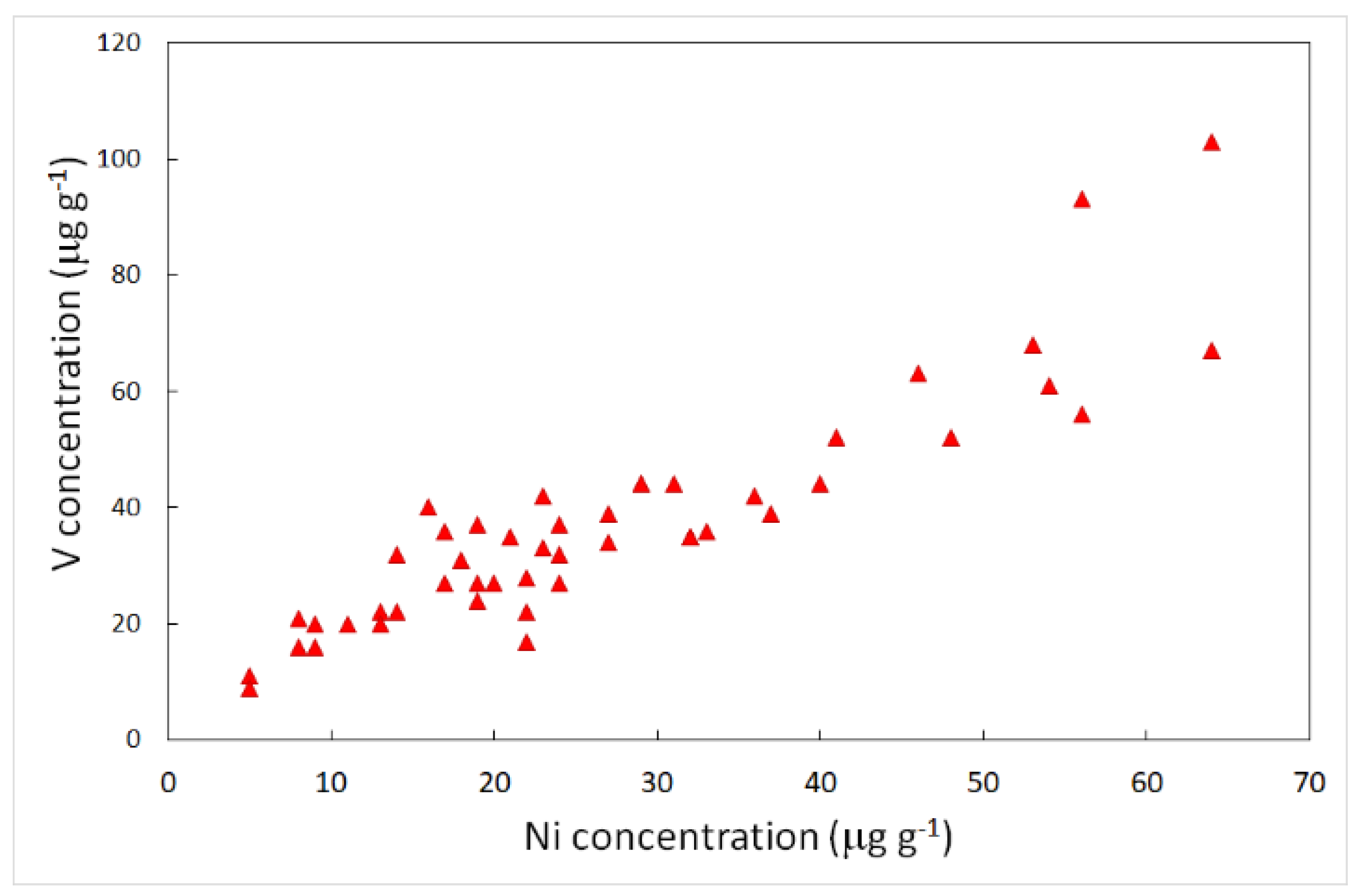
| Ni | 1.00 | 0.42 | −0.18 | 0.59 | 0.10 | 0.52 | −0.07 | 0.87 | 0.55 | |||||||||
| Pb | 1.00 | 0.22 | 0.74 | 0.55 | 0.25 | 0.21 | 0.59 | 0.68 | ||||||||||
| Rb | 1.00 | −0.04 | 0.36 | −0.23 | 0.14 | −0.03 | 0.00 | |||||||||||
| Sb | 1.00 | 0.43 | 0.42 | 0.23 | 0.67 | 0.85 | ||||||||||||
| Sr | 1.00 | 0.49 | 0.20 | 0.19 | 0.43 | |||||||||||||
| Ti | 1.00 | −0.07 | 0.50 | 0.44 | ||||||||||||||
| U | 1.00 | 0.00 | 0.19 | |||||||||||||||
| V | 1.00 | 0.61 | ||||||||||||||||
| Zn | 1.00 |
| Factor 1 | Factor 2 | Factor 3 | Communalities | |
|---|---|---|---|---|
| Anthropic | Anthropic | Geogenic | ||
| Al | 0.28 | 0.19 | 0.90 | 0.90 |
| As | −0.03 | 0.63 | 0.52 | 0.61 |
| Cr | 0.23 | 0.85 | −0.02 | 0.60 |
| Fe | 0.28 | 0.65 | 0.53 | 0.72 |
| Mn | 0.02 | 0.81 | 0.25 | 0.67 |
| Ni | 0.86 | −0.15 | 0.31 | 0.88 |
| Pb | 0.68 | 0.39 | 0.01 | 0.54 |
| Sb | 0.80 | 0.37 | 0.08 | 0.80 |
| Ti | 0.21 | 0.08 | 0.92 | 0.87 |
| V | 0.87 | 0.02 | 0.29 | 0.89 |
| Zn | 0.84 | 0.28 | 0.21 | 0.80 |
| Expl.Var | 3.55 | 2.64 | 2.50 | |
| Prp.Totl | 0.32 | 0.24 | 0.23 |
| As | Cr | Cu | Ni | Pb | Sb | V | Zn | ||
|---|---|---|---|---|---|---|---|---|---|
| CF | 1.39 | 1.38 | 1.21 | 2.63 | 2.03 | 1.94 | 2.23 | 1.75 | |
| ERI | 13.88 | 2.75 | 6.05 | 13.2 | 10.1 | 4.47 | 1.75 | ||
| PLI | 1.76 |
Publisher’s Note: MDPI stays neutral with regard to jurisdictional claims in published maps and institutional affiliations. |
© 2022 by the authors. Licensee MDPI, Basel, Switzerland. This article is an open access article distributed under the terms and conditions of the Creative Commons Attribution (CC BY) license (https://creativecommons.org/licenses/by/4.0/).
Share and Cite
Varrica, D.; Lo Medico, F.; Alaimo, M.G. Air Quality Assessment by the Determination of Trace Elements in Lichens (Xanthoria calcicola) in an Industrial Area (Sicily, Italy). Int. J. Environ. Res. Public Health 2022, 19, 9746. https://doi.org/10.3390/ijerph19159746
Varrica D, Lo Medico F, Alaimo MG. Air Quality Assessment by the Determination of Trace Elements in Lichens (Xanthoria calcicola) in an Industrial Area (Sicily, Italy). International Journal of Environmental Research and Public Health. 2022; 19(15):9746. https://doi.org/10.3390/ijerph19159746
Chicago/Turabian StyleVarrica, Daniela, Federica Lo Medico, and Maria Grazia Alaimo. 2022. "Air Quality Assessment by the Determination of Trace Elements in Lichens (Xanthoria calcicola) in an Industrial Area (Sicily, Italy)" International Journal of Environmental Research and Public Health 19, no. 15: 9746. https://doi.org/10.3390/ijerph19159746
APA StyleVarrica, D., Lo Medico, F., & Alaimo, M. G. (2022). Air Quality Assessment by the Determination of Trace Elements in Lichens (Xanthoria calcicola) in an Industrial Area (Sicily, Italy). International Journal of Environmental Research and Public Health, 19(15), 9746. https://doi.org/10.3390/ijerph19159746