
Temporal and Spatial Changes in the Material Exchange Function of Coastal Intertidal Wetland—A Case Study of Yancheng Intertidal Wetland

Abstract
:1. Introduction
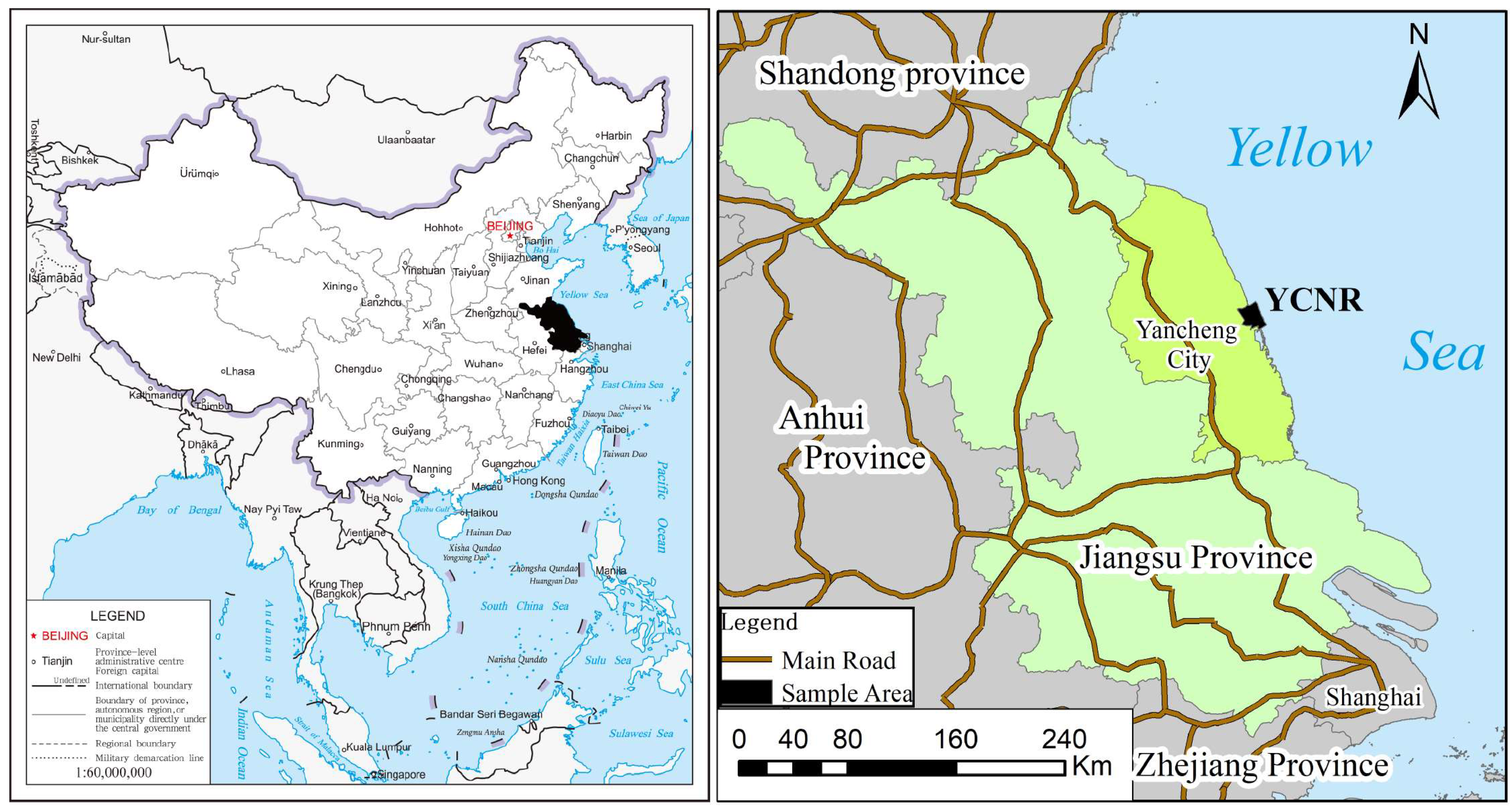
2. Study Area
3. Methods
3.1. Acquisition and Processing of Relevant Data
3.1.1. Wetland Ecosystem Types and Coverage Data
3.1.2. Terrain Data
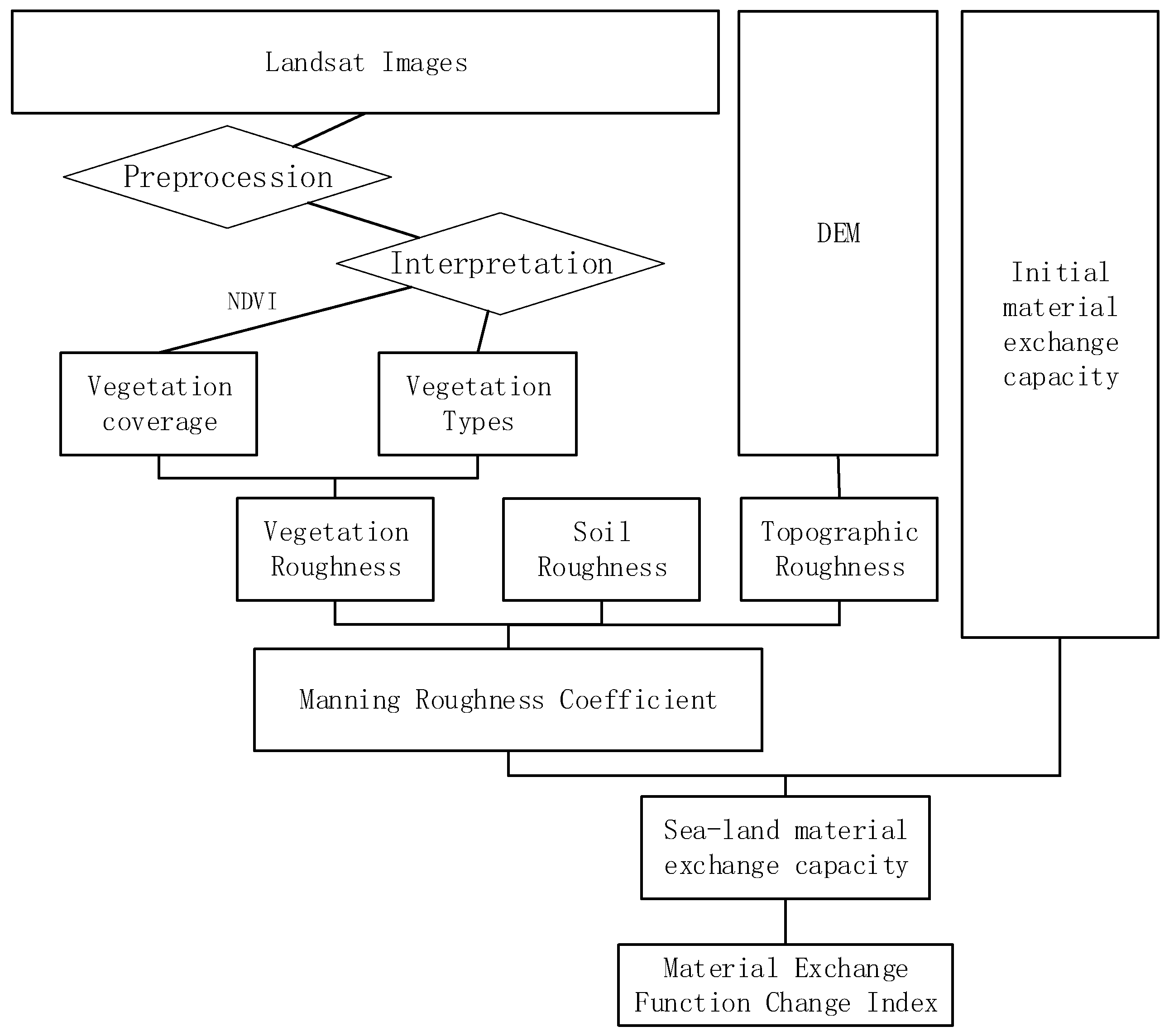
3.2. Construction of the Material Exchange Function Index
3.2.1. Manning Roughness Coefficient
3.2.2. Material Exchange Function Index
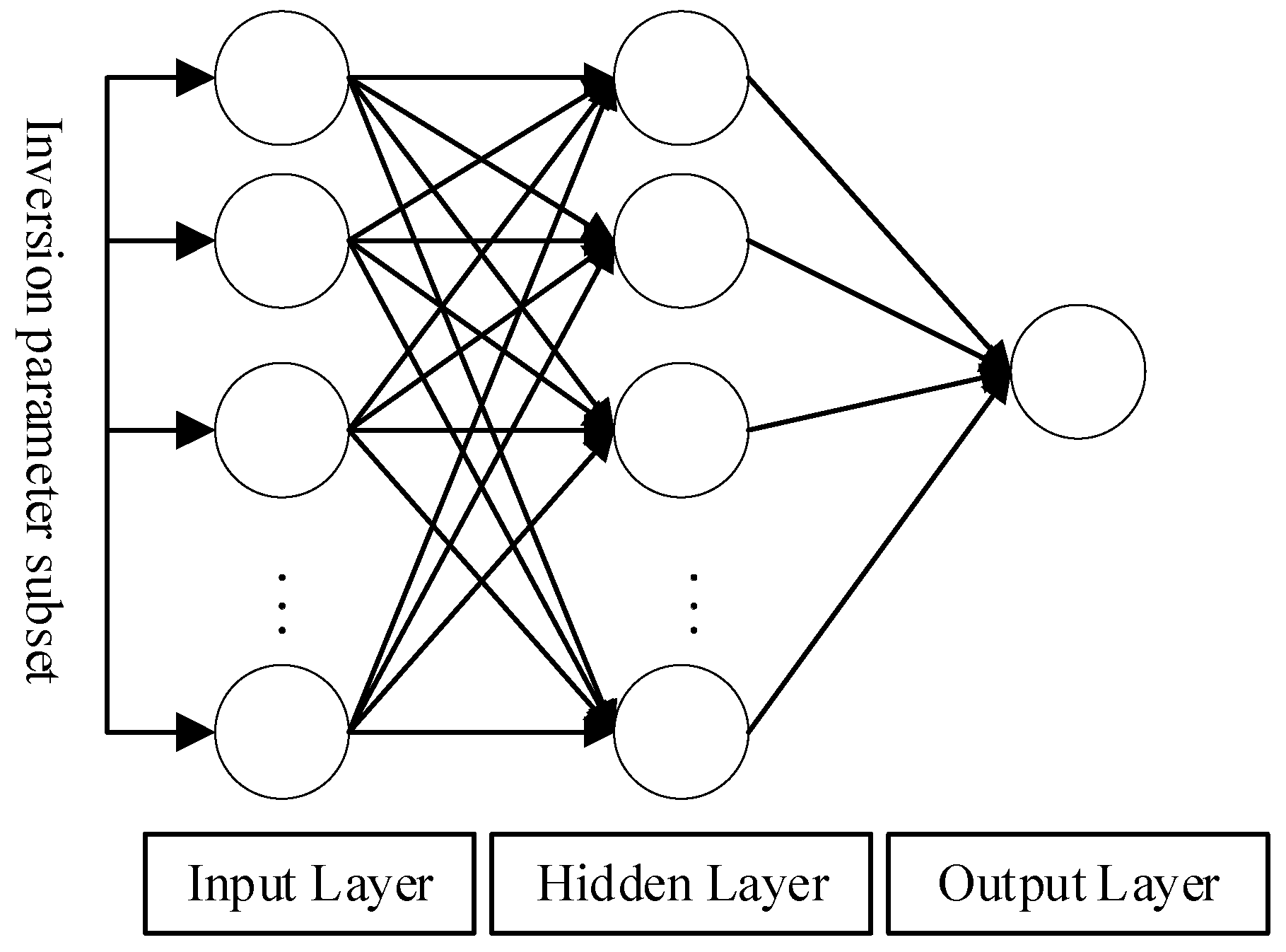
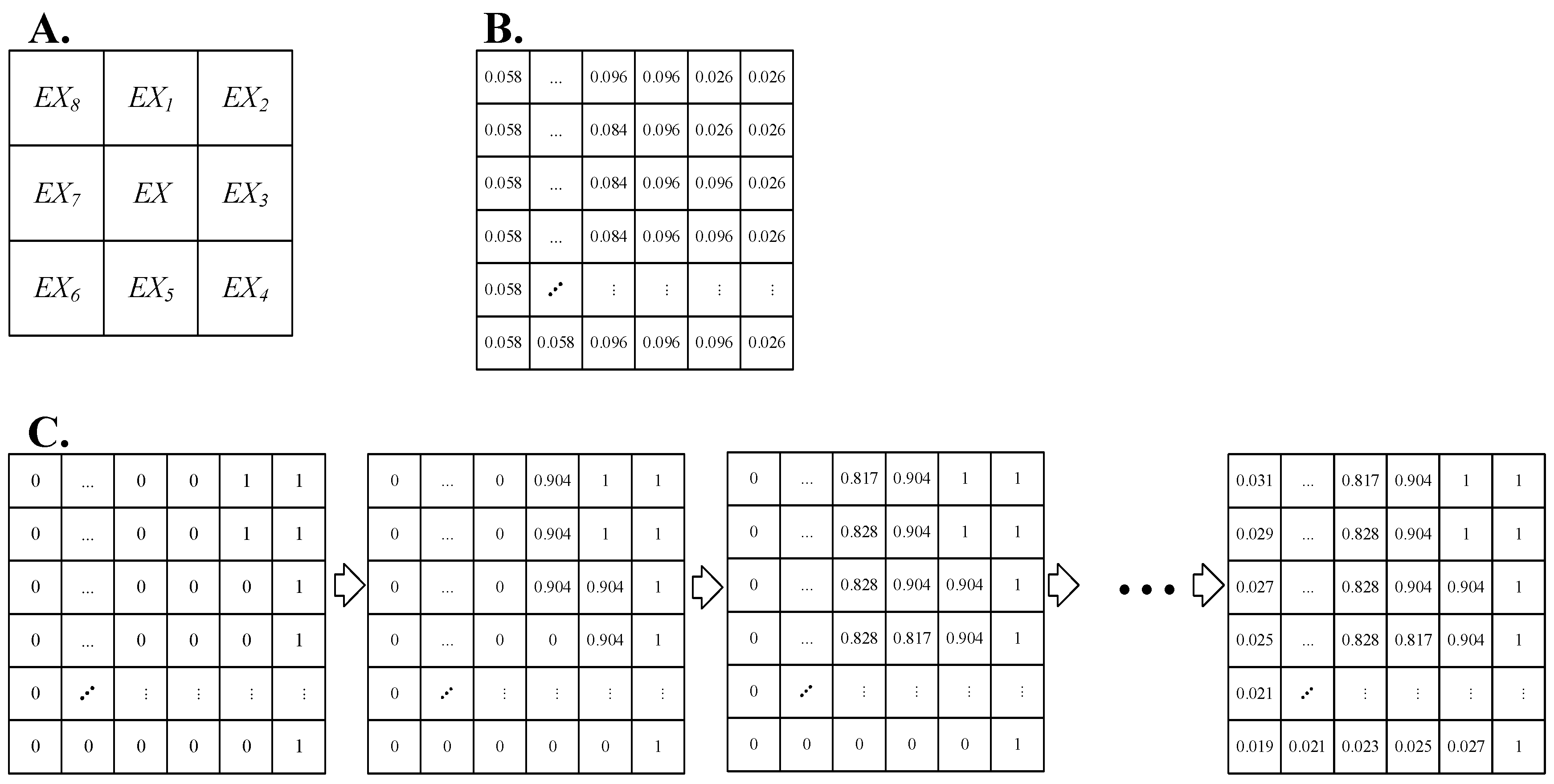
3.3. Methods for Evaluating the Material Exchange Function of the Intertidal Zone
4. Results
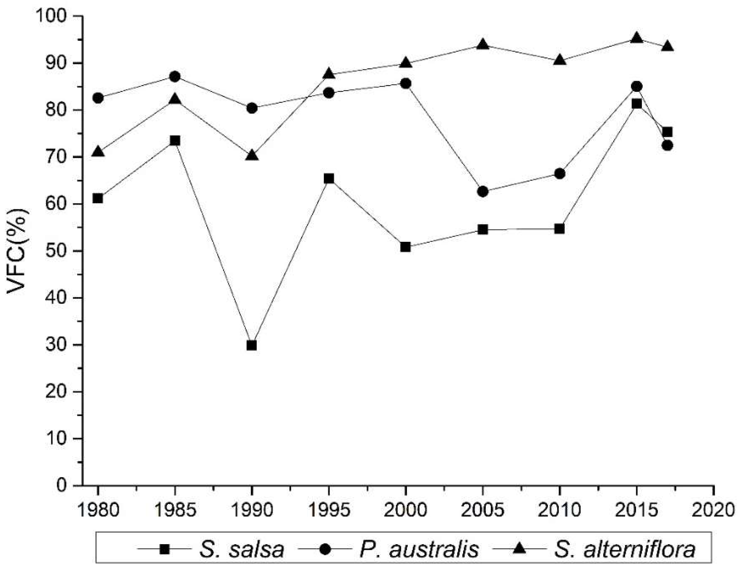
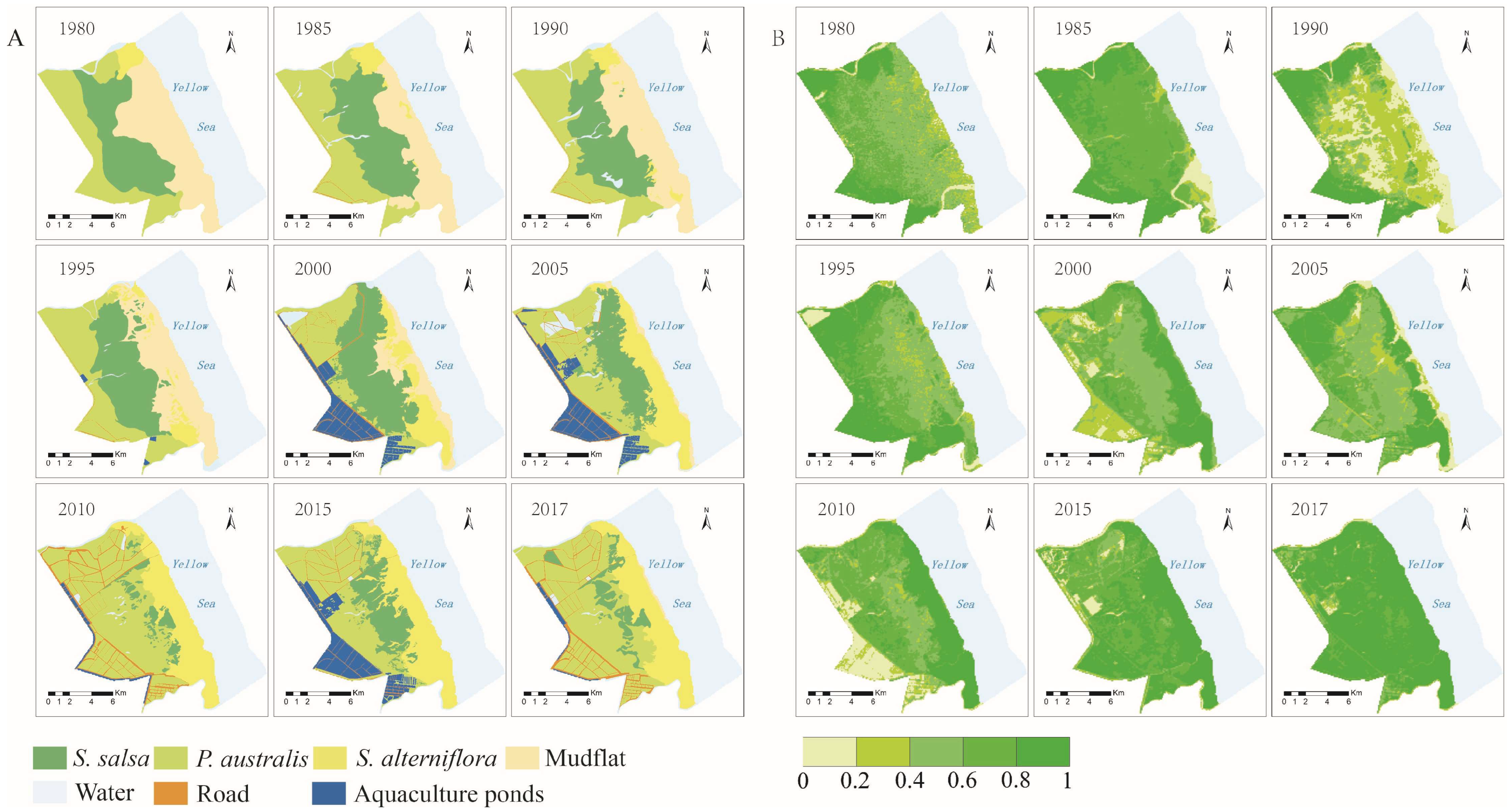
4.1. Spatial Differentiation of Wetland Vegetation Types and Coverage
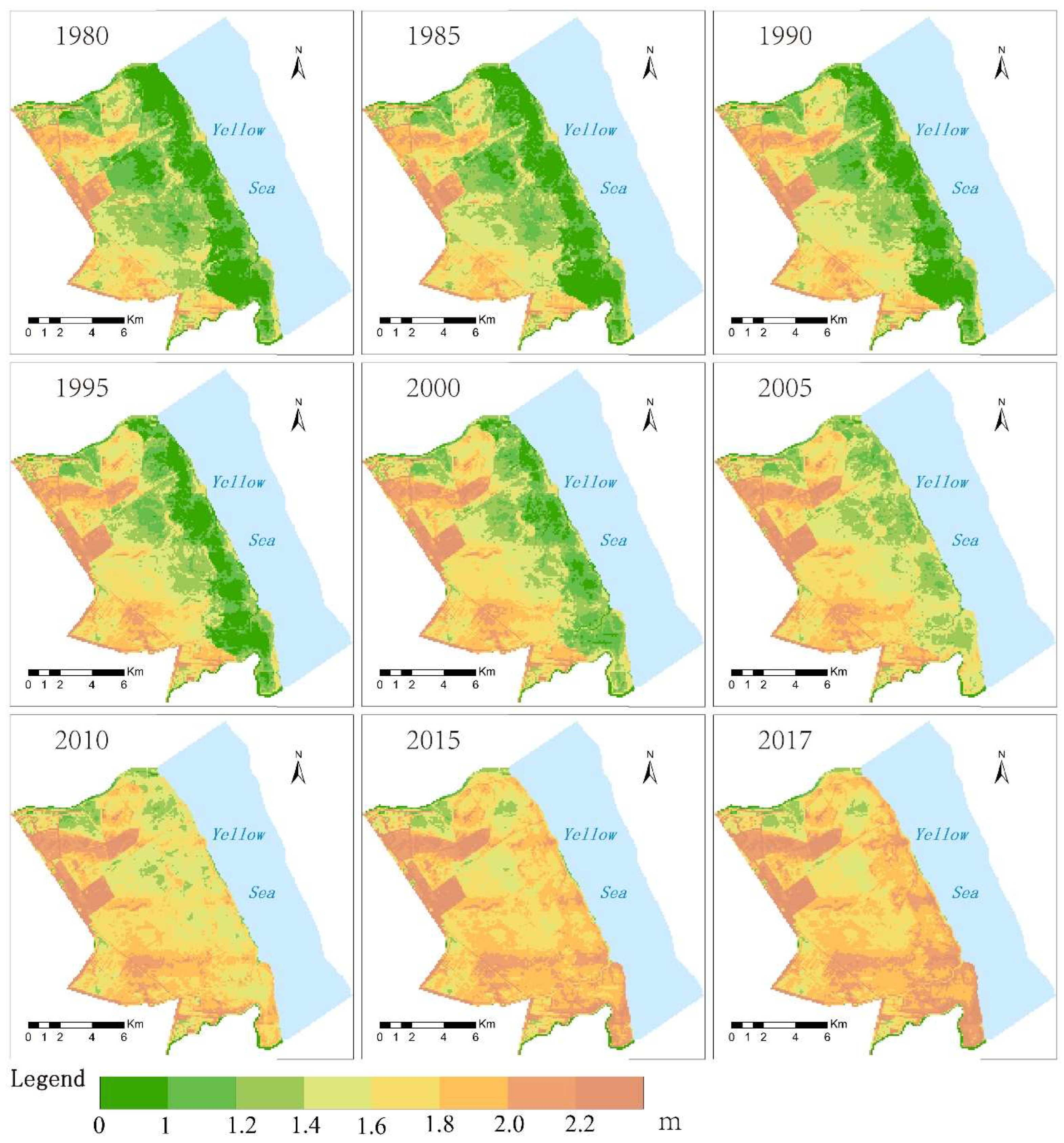
4.2. The Spatial Differentiation Characteristics of the Topography of the Intertidal Zone
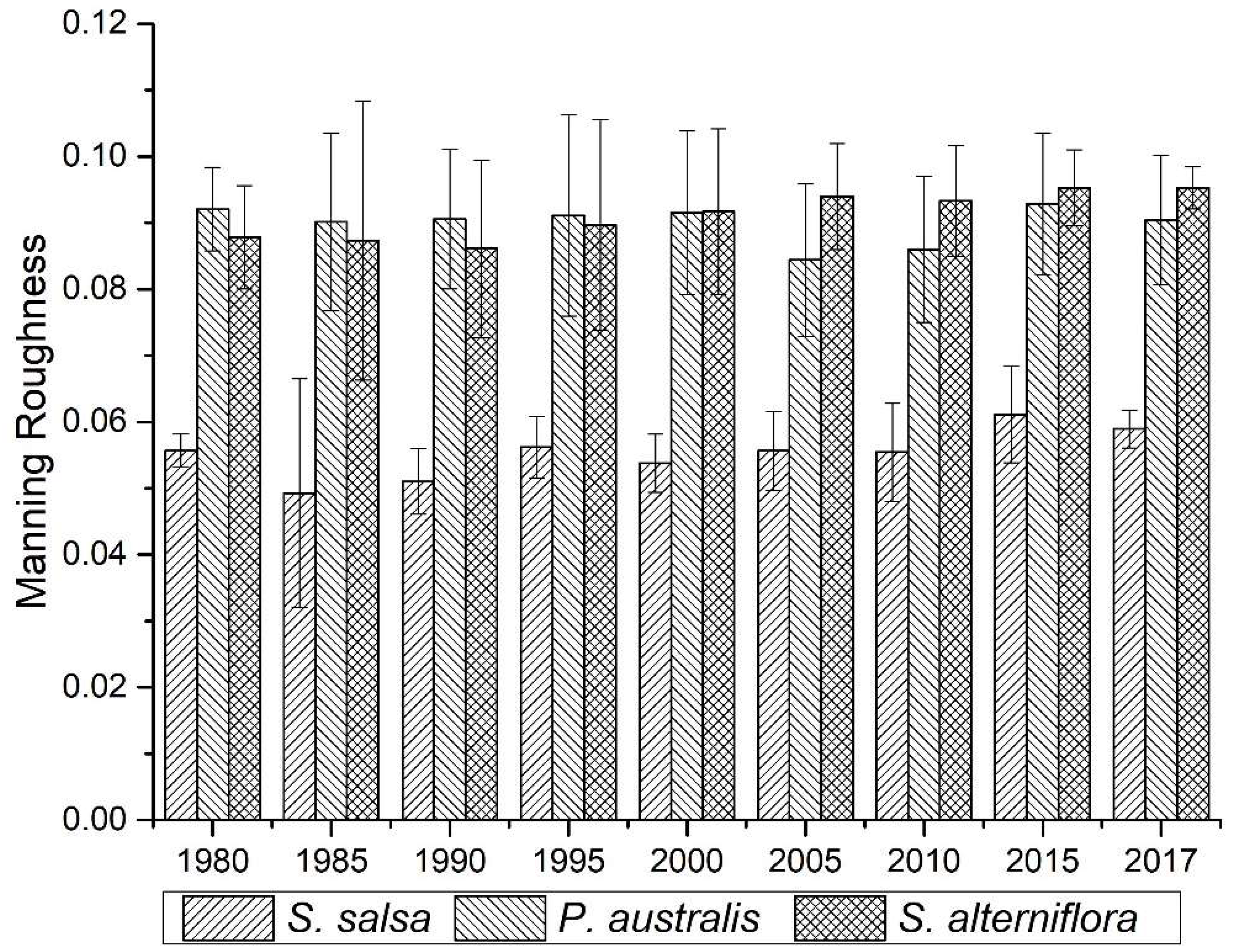
4.3. Spatial Differentiation of the Surface Roughness of Wetland in the Intertidal Zone
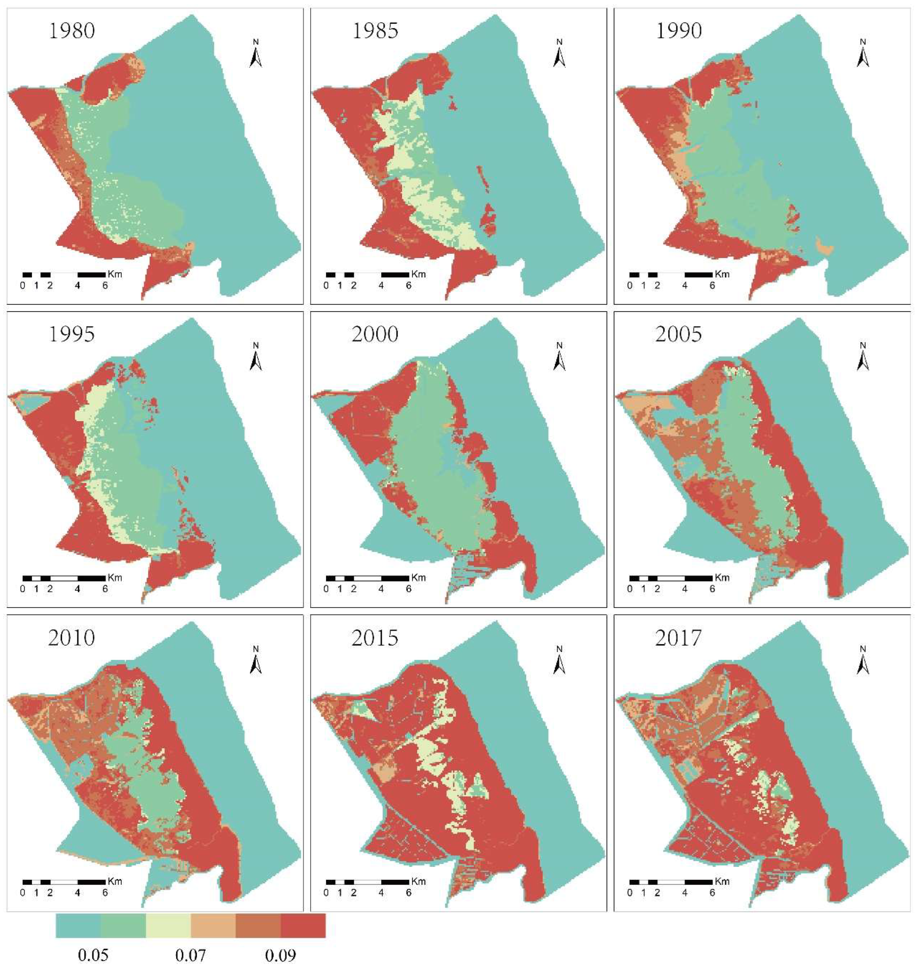
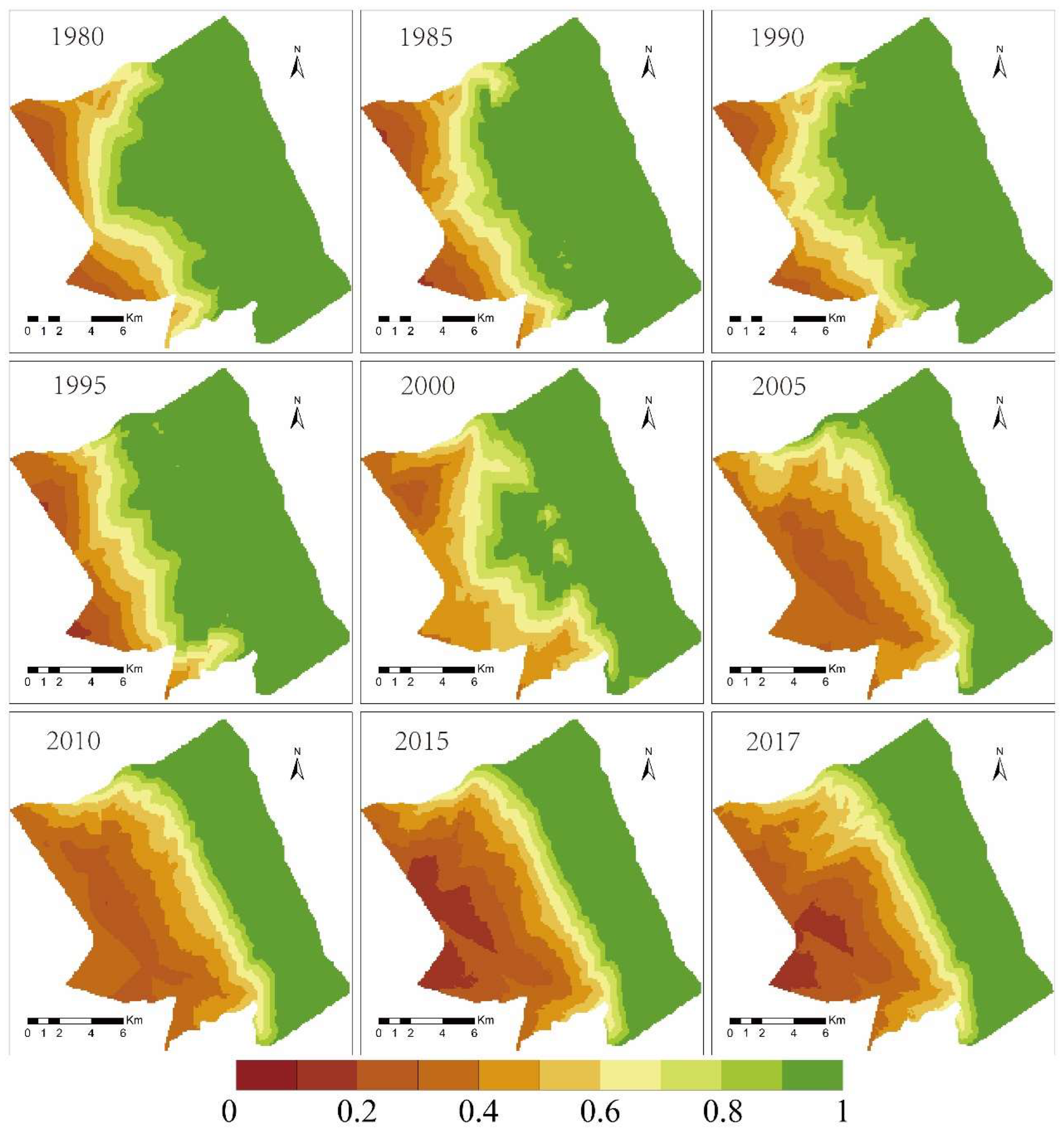
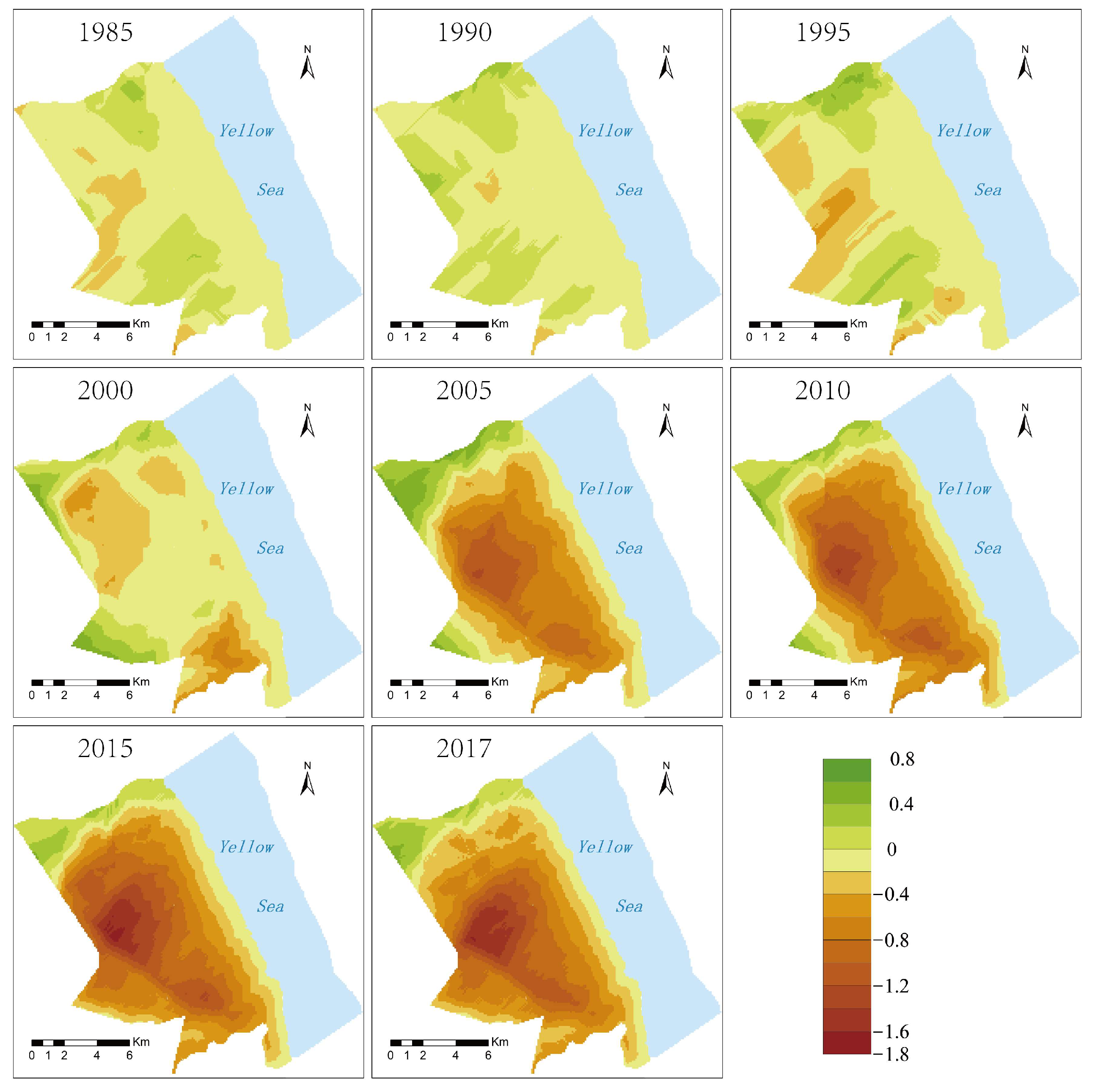
4.4. The Spatial Characteristics and Changes in the Material Exchange Function in the Intertidal Zone
5. Discussion
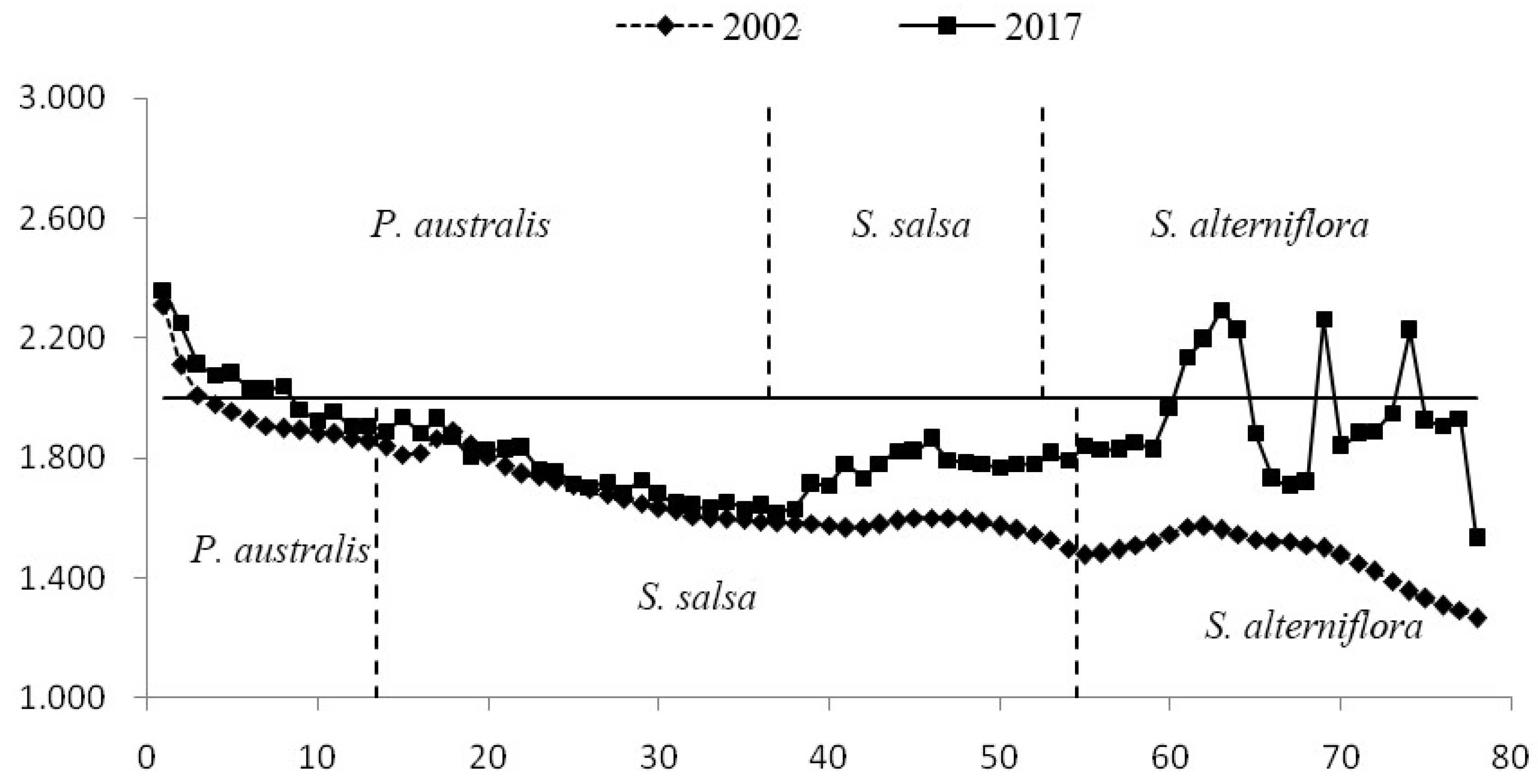
5.1. Influence of S. alterniflora on Hydrological Processes
5.2. Effects of S. alterniflora on the Yancheng Coastal Wetland Ecosystem
5.3. Implications of the Land–Sea Material Exchange Function Model
- Data source: remote sensing data acquisition is affected by weather factors, and obtaining appropriate images is the key. We easily obtained global elevation data with a spatial resolution of 90 m, but more accuracy requires lidar data to provide high-precision elevation information.
- Data accuracy: the spatial resolution of Landsat data was 30 m. In order to improve the accuracy of the results, it is necessary to acquire high-resolution satellite images.
6. Conclusions
- The material exchange function of the wetland ecosystem in the intertidal zone showed a gradual decline from land to sea, and its influencing factors were mainly terrain and vegetation spatial distribution.
- The invasion of S. alterniflora was the main factor in the change in the material exchange function of the wetland in the intertidal zone. The material exchange function of the intertidal zone is an important material guarantee for maintaining the health and natural succession of the wetland ecosystem. Taking the material exchange capacity in 1980 as a reference, the material exchange capacity dropped by 25% in 2017. The size of the area with a high material exchange capacity is decreasing. By 2017, it had been reduced by 71%. In contrast, the size of the area with a low material exchange capacity is increasing; by 2017, it has increased by three times.
Author Contributions
Funding
Institutional Review Board Statement
Informed Consent Statement
Data Availability Statement
Acknowledgments
Conflicts of Interest
References
- Chambers, L.G.; Steinmuller, H.E.; Breithaupt, J.L. Toward a mechanistic understanding of “peat collapse” and its potential contribution to coastal wetland loss. Ecology 2019, 100, 15. [Google Scholar] [CrossRef] [PubMed] [Green Version]
- Yun, C.; Jiang, X. Research on Sustainable Development and Integrated Management of Coastal Zone Ocean; Ocean Press: Beijing, China, 2002. [Google Scholar]
- Sparacino, M.S.; Rathburn, S.L.; Covino, T.P.; Singha, K.; Ronayne, M.J. Form-based river restoration decreases wetland hyporheic exchange: Lessons learned from the Upper Colorado River. Earth Surf. Processes Landf. 2019, 44, 191–203. [Google Scholar] [CrossRef] [Green Version]
- Odum, E.P. Halophytes, energetics and ecosystems. In Ecology of Halophytes; Academic Press: New York, NY, USA, 1974. [Google Scholar]
- Woodwell, G.; Hall, C.; Whitney, D.; Houghton, R. The Flax Pond ecosystem study: Exchanges of inorganic nitrogen between an estuarine marsh and Long Island Sound. Ecology 1979, 60, 695–702. [Google Scholar] [CrossRef]
- Odum, E.P. The status of three ecosystem-level hypotheses regarding salt marsh estuaries: Tidal subsidy, outwelling, and detritus-based food chains. In Estuarine Perspectives; Elsevier: Amsterdam, The Netherlands, 1980; pp. 485–495. [Google Scholar]
- Wolaver, T.G.; Zieman, J.C.; Wetzel, R.; Webb, K.L. Tidal exchange of nitrogen and phosphorus between a mesohaline vegetated marsh and the surrounding estuary in the lower Chesapeake Bay. Estuar. Coast. Shelf Sci. 1983, 16, 321–332. [Google Scholar] [CrossRef]
- DeLaune, R.; Baumann, R.; Gosselink, J. Relationships among vertical accretion, coastal submergence, and erosion in a Louisiana Gulf Coast marsh. J. Sediment. Res. 1983, 53, 147–157. [Google Scholar]
- Cahoon, D.R.; Reed, D.J. Relationships among marsh surface topography, hydroperiod, and soil accretion in a deteriorating Louisiana salt marsh. J. Coast. Res. 1995, 11, 357–369. [Google Scholar]
- Leonard, L.A.; Hine, A.C.; Luther, M.E. Surficial sediment transport and deposition processes in a Juncus roemerianus marsh, west-central Florida. J. Coast. Res. 1995, 11, 322–336. [Google Scholar]
- Leonard, L.A. Controls of sediment transport and deposition in an incised mainland marsh basin, southeastern North Carolina. Wetlands 1997, 17, 263–274. [Google Scholar] [CrossRef]
- Wang, J.; Chen, z.; Wang, D.; Liu, J.; Xu, S. Study on Calculating System of Dissolved Inorganic Nitrogen Exchange Total Fluxes at the Sediment-Water Interface in Yangtze Estuary Tidal Wetlands. Res. Environ. Sci. 2006, 19, 1–7. [Google Scholar]
- Yi, X.; Lu, Y.; Dan, X.; Zhou, G.; Ma, X. Study on Value- Evaluation on the Wetland Benefit Index of Dongjiang Lake Wetland. Cent. South For. Inventory Plan. 2006, 25, 48–51. [Google Scholar]
- Qu, J.; Sun, C. Estimate on wetland parameters and their application—Take CH4 as an example. Territ. Nat. Resour. Study 2001, 17, 42–44. [Google Scholar]
- Lv, G.; Zhou, G.; Zhou, L.; Xie, Y.; Jia, Q.; Zhao, X. Seasonal dynamics of dissolved organic carbon and available N in Panjin reed wetland. J. Meteorol. Environ. 2006, 22, 59–63. [Google Scholar]
- Meng, W. Diagnosis Technology of Coastal Habitat Degradation Science; China Science Publishing: Beijing, China, 2009. [Google Scholar]
- Gao, Y.; Peng, R.H.; Ouyang, Z.T.; Shao, C.L.; Chen, J.Q.; Zhang, T.T.; Guo, H.Q.; Tang, J.W.; Zhao, F.; Zhuang, P.; et al. Enhanced Lateral Exchange of Carbon and Nitrogen in a Coastal Wetland With Invasive Spartina alterniflora. J. Geophys. Res. Biogeosci. 2020, 125, e2019JG005459. [Google Scholar] [CrossRef]
- Murray, K.R.; Borkenhagen, A.K.; Cooper, D.J.; Strack, M. Growing season carbon gas exchange from peatlands used as a source of vegetation donor material for restoration. Wetl. Ecol. Manag. 2017, 25, 501–515. [Google Scholar] [CrossRef]
- Kastler, J.; Wiberg, P. Sedimentation and Boundary Changes of Virginia Salt Marshes. Estuar. Coast. Shelf Sci. 1996, 42, 683–700. [Google Scholar] [CrossRef]
- Nunez, K.; Zhang, Y.L.J.; Herman, J.; Reay, W.; Hershner, C. A multi-scale approach for simulating tidal marsh evolution. Ocean. Dyn. 2020, 70, 1187–1209. [Google Scholar] [CrossRef]
- Sorensen, R.M. Water waves produced by ships. J. Waterw. Harb. Coast. Eng. Div. 1973, 99, 245–256. [Google Scholar] [CrossRef]
- Makungu, E.; Hughes, D.A. Understanding and modelling the effects of wetland on the hydrology and water resources of large African river basins. J. Hydrol. 2021, 603, 127039. [Google Scholar] [CrossRef]
- Chu, X.J.; Han, G.X.; Xing, Q.H.; Xia, J.Y.; Sun, B.Y.; Li, X.G.; Yu, J.B.; Li, D.J.; Song, W.M. Changes in plant biomass induced by soil moisture variability drive interannual variation in the net ecosystem CO2 exchange over a reclaimed coastal wetland. Agric. For. Meteorol. 2019, 264, 138–148. [Google Scholar] [CrossRef]
- Wayne, C. The effects of sea and marsh grass on wave energy. Coast. Res. Notes 1976, 4, 6–8. [Google Scholar]
- Knutson, P.; Ford, J.; Inskeep, M.; Oyler, J. National survey of planted salt marshes (Vegetative stabilization and wave stress). Wetlands 1981, 1, 129–157. [Google Scholar] [CrossRef]
- XIE, B.; HAN, G. Control of invasive Spartina alterniflora: A review. Chin. J. Appl. Ecol. 2018, 29, 3464–3476. [Google Scholar]
- Yang, W.; An, S.; Zhao, H.; Xu, L.; Qiao, Y.; Cheng, X. Impacts of Spartina alterniflora invasion on soil organic carbon and nitrogen pools sizes, stability, and turnover in a coastal salt marsh of eastern China. Ecol. Eng. 2016, 86, 174–182. [Google Scholar] [CrossRef]
- Xiangzhen, Q.; Huiyu, L.; Zhenshan, L.; Xiang, L.; Haibo, G. Impacts of Age and Expansion Direction of Invasive Spartina alterniflora on Soil Organic Carbon Dynamics in Coastal Salt Marshes Along Eastern China. Estuaries Coasts 2019, 7, 1858–1867. [Google Scholar] [CrossRef]
- Zhang, G.; Bai, J.; Zhao, Q.; Jia, J.; Wang, W.; Wang, X. Bacterial Succession in Salt Marsh Soils Along a Short-term Invasion Chronosequence of Spartina alterniflora in the Yellow River Estuary, China. Microb. Ecol. 2020, 79, 644–661. [Google Scholar] [CrossRef]
- Yang, W.; Zhang, D.; Cai, X.; Xia, L.; Luo, Y.; Cheng, X.; An, S. Significant alterations in soil fungal communities along a chronosequence of Spartina alterniflora invasion in a Chinese Yellow Sea coastal wetland. Sci. Total Environ. 2019, 693, 133548. [Google Scholar] [CrossRef]
- Yanga, W.; Jeelanib, N.; Zhua, Z.; Luoc, Y.; Chengd, X. Alterations in soil bacterial community in relation to Spartina alterniflora Loisel. invasion chronosequence in the eastern Chinese coastal wetlands. Appl. Soil Ecol. 2018, 135, 38–43. [Google Scholar] [CrossRef]
- Ayres, D.R.; Grotkopp, E.; Zaremba, K.; Sloop, C.M.; Blum, M.J.; Bailey, J.P.; Anttila, C.K.; Strong, D.R. Hybridization between invasive Spartina densiflora (Poaceae) and native S. foliosa in San Francisco Bay, California, USA. Am. J. Bot. 2007, 95, 713–719. [Google Scholar] [CrossRef] [PubMed]
- Dackombe, R.; Gardiner, V. Geomorphological Field Manual; Routledge: London, UK, 2020; Volume 12. [Google Scholar]
- Williams, T.P.; Bubb, J.M.; Lester, J.N. Metal accumulation within salt marsh environments: A review. Mar. Pollut. Bull. 1994, 28, 277–290. [Google Scholar] [CrossRef]
- Schwartz, M.L. Encyclopedia of Coastal Science. J. Coast. Res. 2005, 21, 35–36. [Google Scholar]
- Nixon, S.W. Between Coastal Marshes and Coastal Waters—A Review of Twenty Years of Speculation and Research on the Role of Salt Marshes in Estuarine Productivity and Water Chemistry. In Estuarine and Wetland Processes; Springer: Berlin/Heidelberg, Germany, 1980. [Google Scholar]
- De Deyn, G.B.; Cornelissen, J.H.C.; Bardgett, R.D. Plant functional traits and soil carbon sequestration in contrasting biomes. Ecol. Lett. 2008, 11, 516–531. [Google Scholar] [CrossRef]
- Gao, J.; Bai, F.; Yang, Y.; Gao, S.; Liu, Z.; Li, J. Influence of Spartina Colonization on the Supply and Accumulation of Organic Carbon in Tidal Salt Marshes of Northern Jiangsu Province, China. J. Coast. Res. 2012, 28, 486–498. [Google Scholar] [CrossRef]
- Cheng, X.; Luo, Y.; Xu, Q.; Lin, G.; Zhang, Q.; Chen, J.; Li, B. Seasonal variation in CH4 emission and its 13C-isotopic signature from Spartina alterniflora and Scirpus mariqueter soils in an estuarine wetland. Plant Soil 2010, 327, 85–94. [Google Scholar] [CrossRef] [Green Version]
- Li, B. Spartina alterniflora invasions in the Yangtze River estuary, China: An overview of current status and ecosystem effects. Ecol. Eng. 2009, 35, 511–520. [Google Scholar] [CrossRef]
- Liu, Y.; Li, M.; Zhang, R. Approach on the Dynamic Change and Influence Factors of Spartina alterniflora Loisel Salt-marsh along the coast of the Jiangsu Province. Wetl. Sci. 2004, 2, 116–121. [Google Scholar]
- Zhang, R.; Shen, Y.; Lu, L.; Yan, S.; Wang, Y.; Li, J.; Zhang, Z. Formation of Spartina alterniflora salt marsh on Jiangsu coast, China. Oceanol. Limnol. Sin. 2005, 36, 358–366. [Google Scholar]
- Yuan, H.; Li, S.; Zheng, H.; Fang, Z. Evaluation of the influences of foreign Spartina alterniflora on ecosystem of Chinese coastal wetland and its countermeasures. Mar. Sci. Bull. 2009, 28, 122–128. [Google Scholar]
- Wang, J.; Liu, H.; Li, Y.; Liu, L.; Xie, F.; Lou, C.; Zhang, H. Effects of Spartina alterniflora invasion on quality of the red-crowned crane (Grus japonensis) wintering habitat. Environ. Sci. Pollut. Res. 2019, 26, 21546–21555. [Google Scholar] [CrossRef] [PubMed]
- Wang, J. Effects of Spartina Alterniflora Invasion on Quality of the Red-Crowned Crane (Grus japonensis) Wintering Habitat on Yancheng Tidal Wetland. Ph.D. Thesis, Nanjing Normal University, Nanjing, China, 2020. [Google Scholar]
- Tan, Q. Landscape Classification and Biomass Estimation of Typical Coastal Wetlands in Yancheng. Master’s Thesis, Nanjing Normal University, Nanjing, China, 2014. [Google Scholar]
- Zhang, H.B.; Wu, F.E.; Zhang, Y.N.; Han, S.; Liu, Y.Q. Spatial and Temporal Changes of Habitat Quality in Jiangsu Yancheng Wetland National Nature Reserve—Rare Birds of China. Appl. Ecol. Environ. Res. 2019, 17, 4807–4821. [Google Scholar] [CrossRef]
- Zhang, Y.; Ding, W.; Luo, J.; Donnison, A. Changes in Soil Organic Carbon Dynamics in an Eastern Chinese Coastal Wetland Following Invasion by a C4 Plant Spartina alterniflora. Soil Biol. Biochem. 2010, 42, 1712–1720. [Google Scholar] [CrossRef]
- Froelich, P.N. Analysis Of Organic-Carbon In Marine-Sediments. Limnol. Oceanogr. 1980, 25, 564–572. [Google Scholar]


| Year | Sensor | Date | Spatial Resolution/m | Cloudiness/% | Data Identification |
|---|---|---|---|---|---|
| 1980 | MSS | 28 October 1980 | 78 | 0 | LM31280371980302AAA03 |
| 1985 | TM | 24 September 1985 | 30 | 3 | LT51190371985267HAJ00 |
| 1990 | TM | 8 October 1990 | 30 | 8 | LT51190371990281HAJ00 |
| 1995 | TM | 9 December 1995 | 30 | 1 | LT51190371995343CLT00 |
| 2000 | ETM+ | 9 September 2000 | 30 | 53 * | LE71190372000253EDC01 |
| 2005 | ETM+ | 26 November 2005 | 30 | 6 | LE71190372005330EDC00 |
| 2010 | ETM+ | 10 December 2010 | 30 | 1 | LE71190372010344EDC00 |
| 2015 | OLI | 13 October 2015 | 30 | 0.04 | LC81190372015286LGN01 |
| 2017 | OLI | 5 December 2017 | 30 | 0.58 | LC81190372017339LGN00 |
| Roughness Value | Feature Description | |||
|---|---|---|---|---|
| 0.025 | Wetland bare soil background value | |||
| 0.030 | Covered by gravel and broken shells in more than 25% of area | |||
| 0.001 | A typical flat area without micro-landforms (such as hills) or large-scale landforms (such as narrow channels, tidal channels, mountains, depressions, and ponds) | |||
| Vegetation coverage | ||||
| <50% | 50~75% | ≥75% | ||
| 0.025 | 0.030 | 0.035 | Short-stemmed soft-leaf area (S. salsa) | |
| 0.050 | 0.060 | 0.070 | High-stemmed and soft-leaf area (P. australis, S. alterniflora) | |
| Year | S. salsa | P. australis | S. alterniflora | ||||||
|---|---|---|---|---|---|---|---|---|---|
| Min | Max | Mean | Min | Max | Mean | Min | Max | Mean | |
| 1980 | 0.33 | 2.72 | 1.42 | −0.97 | 4.36 | 1.71 | −0.07 | 1.59 | 0.73 |
| 1985 | 0.42 | 2.23 | 1.34 | −1.00 | 4.40 | 1.73 | 0.19 | 1.84 | 0.91 |
| 1990 | −0.84 | 2.96 | 1.52 | −0.96 | 4.43 | 1.78 | 0.40 | 1.87 | 1.06 |
| 1995 | 0.57 | 3.04 | 1.60 | −0.61 | 4.47 | 1.82 | 0.53 | 2.16 | 1.08 |
| 2000 | 0.71 | 2.57 | 1.57 | 0.20 | 4.43 | 1.77 | −0.64 | 2.20 | 1.16 |
| 2005 | 0.95 | 2.61 | 1.54 | 0.20 | 4.46 | 1.78 | 0.91 | 2.32 | 1.40 |
| 2010 | 1.13 | 2.16 | 1.63 | −0.23 | 4.50 | 1.82 | −0.43 | 2.28 | 1.65 |
| 2015 | 1.19 | 2.11 | 1.66 | 0.88 | 4.54 | 1.85 | 0.30 | 2.53 | 1.88 |
| 2017 | 1.26 | 2.26 | 1.72 | 0.51 | 4.47 | 1.85 | 0.71 | 2.63 | 1.97 |
| Mean | 0.63 | 2.52 | 1.56 | −0.22 | 4.45 | 1.79 | 0.21 | 2.16 | 1.32 |
| Years | Material Exchange Function | |||||||||
|---|---|---|---|---|---|---|---|---|---|---|
| 0.1–0.2 | 0.2–0.3 | 0.3–0.4 | 0.4–0.5 | 0.5–0.6 | 0.6–0.7 | 0.7–0.8 | 0.8–0.9 | 0.9–1 | ||
| 1980 | S. alterniflora | 0.66 | 1.41 | 1.84 | 1.56 | |||||
| S. salsa | 2.68 | 6.69 | 7.78 | 9.38 | 10.76 | 9.08 | ||||
| P. australis | 0.06 | 6.88 | 10.23 | 8.94 | 8.39 | 6 | 2.76 | 1.31 | 0.94 | |
| 1985 | S. alterniflora | 1.06 | 1.88 | 2.05 | 3.46 | |||||
| S. salsa | 0.38 | 4.04 | 8.92 | 9.23 | 8.15 | 7.45 | ||||
| P. australis | 0.76 | 9.85 | 10.13 | 12.03 | 9.36 | 3.92 | 2.4 | 1.83 | 0.81 | |
| 1990 | S. alterniflora | 0.22 | 1.07 | 1.6 | 3.58 | |||||
| S. salsa | 0.08 | 3.08 | 8.95 | 12.94 | 11.04 | 10.45 | ||||
| P. australis | 0.04 | 6.05 | 9.74 | 10.45 | 11.61 | 6.9 | 2.73 | 1.29 | 0.73 | |
| 1995 | S. alterniflora | 0.5 | 1.19 | 1.7 | 5.93 | |||||
| S. salsa | 1.16 | 7.28 | 8.9 | 10.07 | 9.62 | 11.39 | ||||
| P. australis | 1.22 | 7.91 | 13.77 | 10.58 | 5.79 | 4.06 | 2.37 | 1.37 | 0.42 | |
| 2000 | S. alterniflora | 0.47 | 1.69 | 2.12 | 3.61 | 6.37 | 7.79 | |||
| S. salsa | 0.73 | 6.4 | 12.85 | 14.3 | 10.56 | 8.53 | ||||
| P. australis | 3.09 | 8.14 | 10.17 | 8.03 | 2.41 | 0.64 | ||||
| 2005 | S. alterniflora | 0.62 | 2.01 | 4.04 | 5.55 | 8.02 | 7.66 | 5.93 | ||
| S. salsa | 1.3 | 3.69 | 12.21 | 9.88 | 4.72 | 1.77 | 1.19 | 0.15 | ||
| P. australis | 10.45 | 17.78 | 10.84 | 4.72 | 3.01 | 1.79 | 0.76 | 0.15 | ||
| 2010 | S. alterniflora | 0.01 | 1.65 | 4.85 | 6.06 | 7.04 | 9.19 | 8.12 | 5.66 | |
| S. salsa | 0.35 | 7.36 | 10.55 | 6.22 | 2.45 | 0.77 | 0.21 | |||
| P. australis | 0.02 | 18.85 | 22.06 | 8.09 | 4.02 | 2.63 | 0.91 | 0.08 | 0.11 | |
| 2015 | S. alterniflora | 1.01 | 3.08 | 6.13 | 6.85 | 9.47 | 7.94 | 5.27 | ||
| S. salsa | 1.47 | 5.76 | 4.19 | 1.77 | 1.98 | 0.42 | 0.25 | 0.01 | ||
| P. australis | 15.18 | 27.72 | 20.27 | 13.04 | 4.76 | 2.19 | 0.69 | 0.05 | ||
| 2017 | S. alterniflora | 0.63 | 3.19 | 5.75 | 6.94 | 9.17 | 8.07 | 5.22 | ||
| S. salsa | 0.11 | 2.51 | 3.6 | 2.33 | 1.2 | 0.28 | ||||
| P. australis | 9.6 | 26 | 22.23 | 16.92 | 7.61 | 3.91 | 1.08 | 0.21 | 0.01 | |
Publisher’s Note: MDPI stays neutral with regard to jurisdictional claims in published maps and institutional affiliations. |
© 2022 by the authors. Licensee MDPI, Basel, Switzerland. This article is an open access article distributed under the terms and conditions of the Creative Commons Attribution (CC BY) license (https://creativecommons.org/licenses/by/4.0/).
Share and Cite
Dai, L.; Liu, H.; Li, Y. Temporal and Spatial Changes in the Material Exchange Function of Coastal Intertidal Wetland—A Case Study of Yancheng Intertidal Wetland. Int. J. Environ. Res. Public Health 2022, 19, 9419. https://doi.org/10.3390/ijerph19159419
Dai L, Liu H, Li Y. Temporal and Spatial Changes in the Material Exchange Function of Coastal Intertidal Wetland—A Case Study of Yancheng Intertidal Wetland. International Journal of Environmental Research and Public Health. 2022; 19(15):9419. https://doi.org/10.3390/ijerph19159419
Chicago/Turabian StyleDai, Lingjun, Hongyu Liu, and Yufeng Li. 2022. "Temporal and Spatial Changes in the Material Exchange Function of Coastal Intertidal Wetland—A Case Study of Yancheng Intertidal Wetland" International Journal of Environmental Research and Public Health 19, no. 15: 9419. https://doi.org/10.3390/ijerph19159419
APA StyleDai, L., Liu, H., & Li, Y. (2022). Temporal and Spatial Changes in the Material Exchange Function of Coastal Intertidal Wetland—A Case Study of Yancheng Intertidal Wetland. International Journal of Environmental Research and Public Health, 19(15), 9419. https://doi.org/10.3390/ijerph19159419