
Mapping Building-Based Spatiotemporal Distributions of Carbon Dioxide Emission: A Case Study in England


Abstract
:1. Introduction
2. Materials and Methods
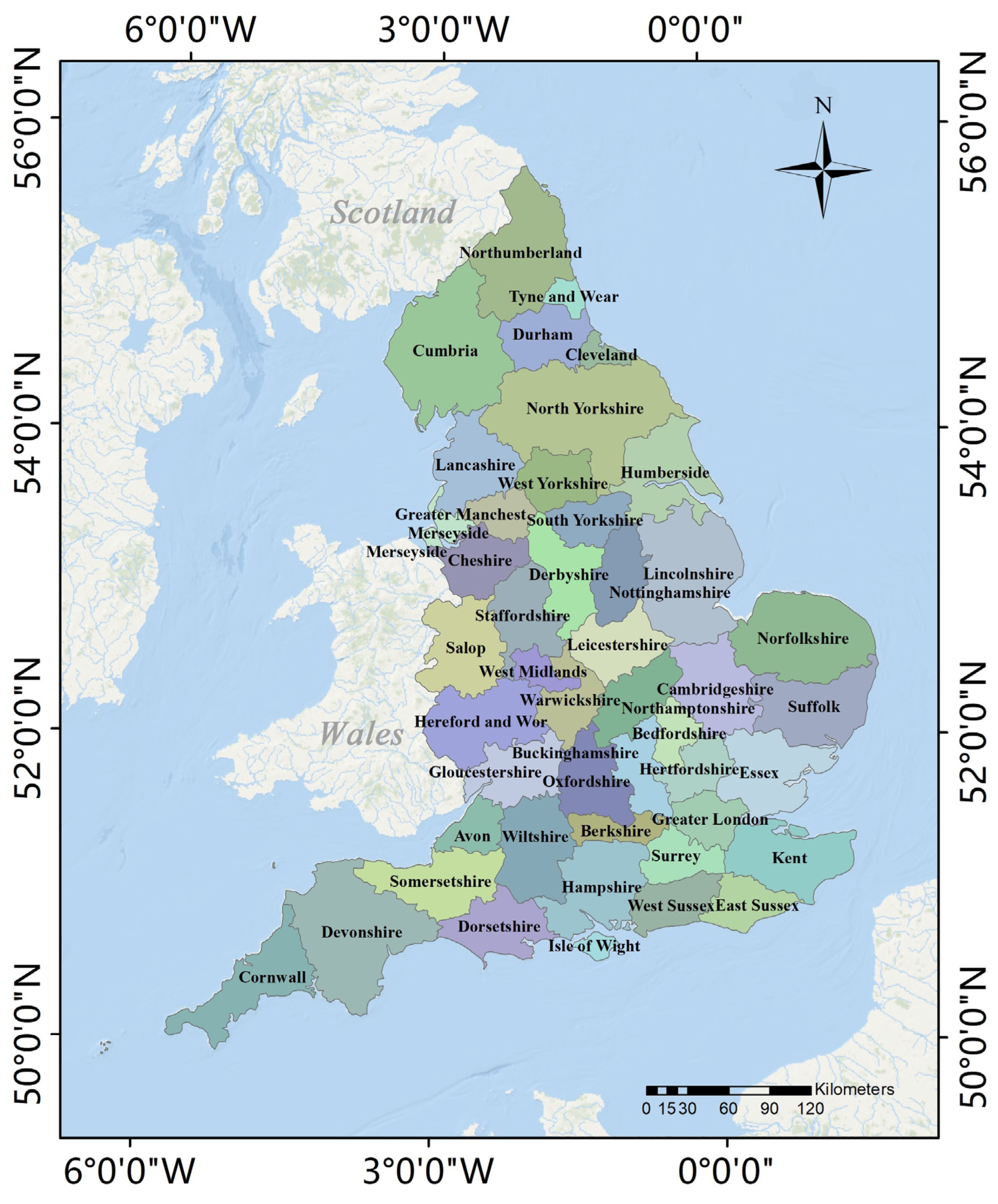
2.1. Study Area
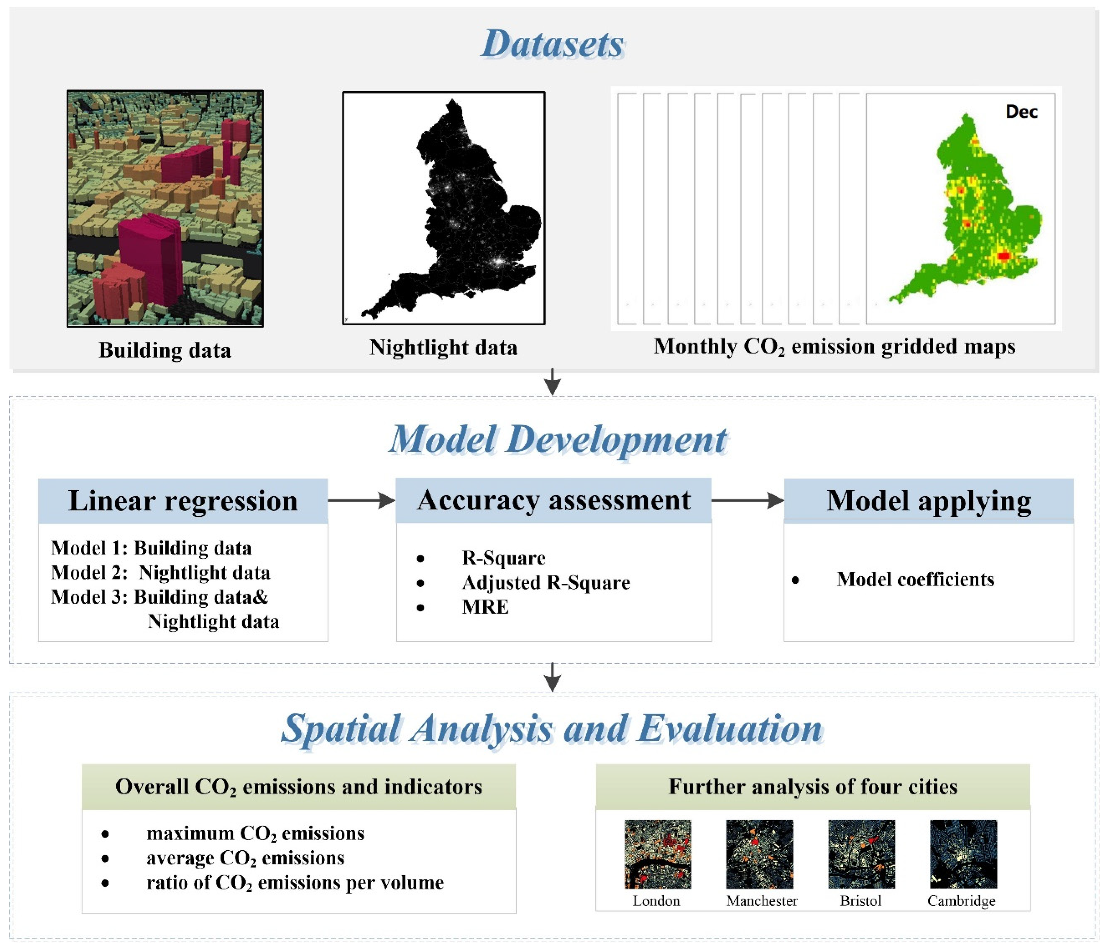
2.2. Overall Framework
2.3. Data Preparation and Processing
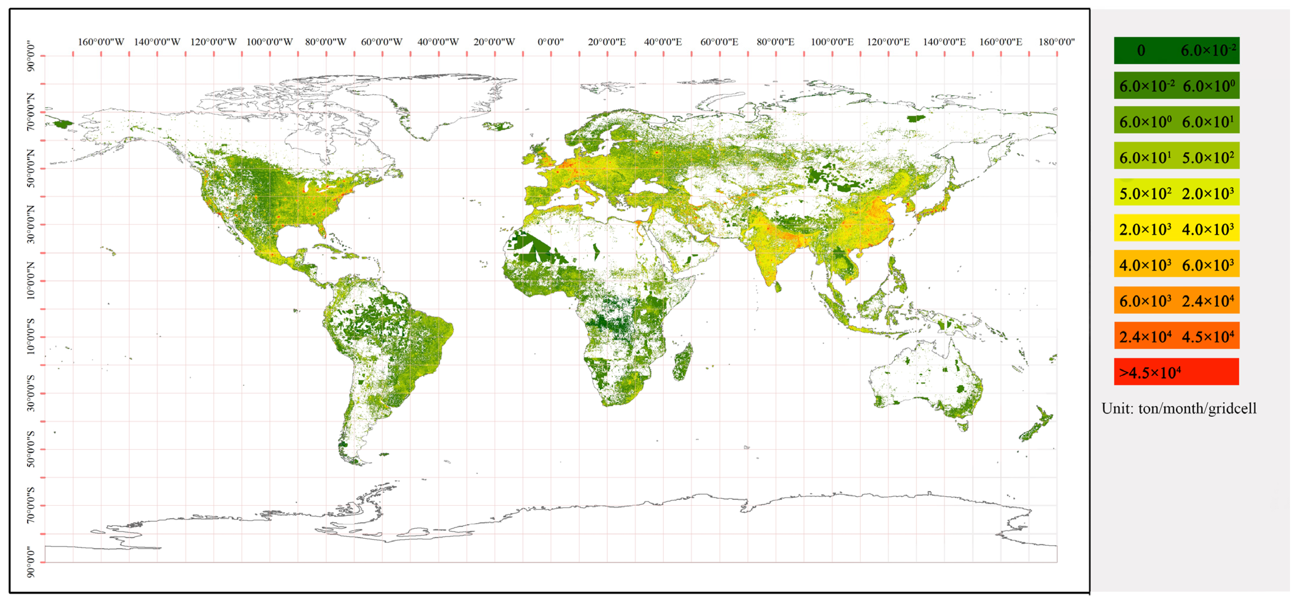
2.3.1. Monthly CO2 Emissions Data from EDGAR
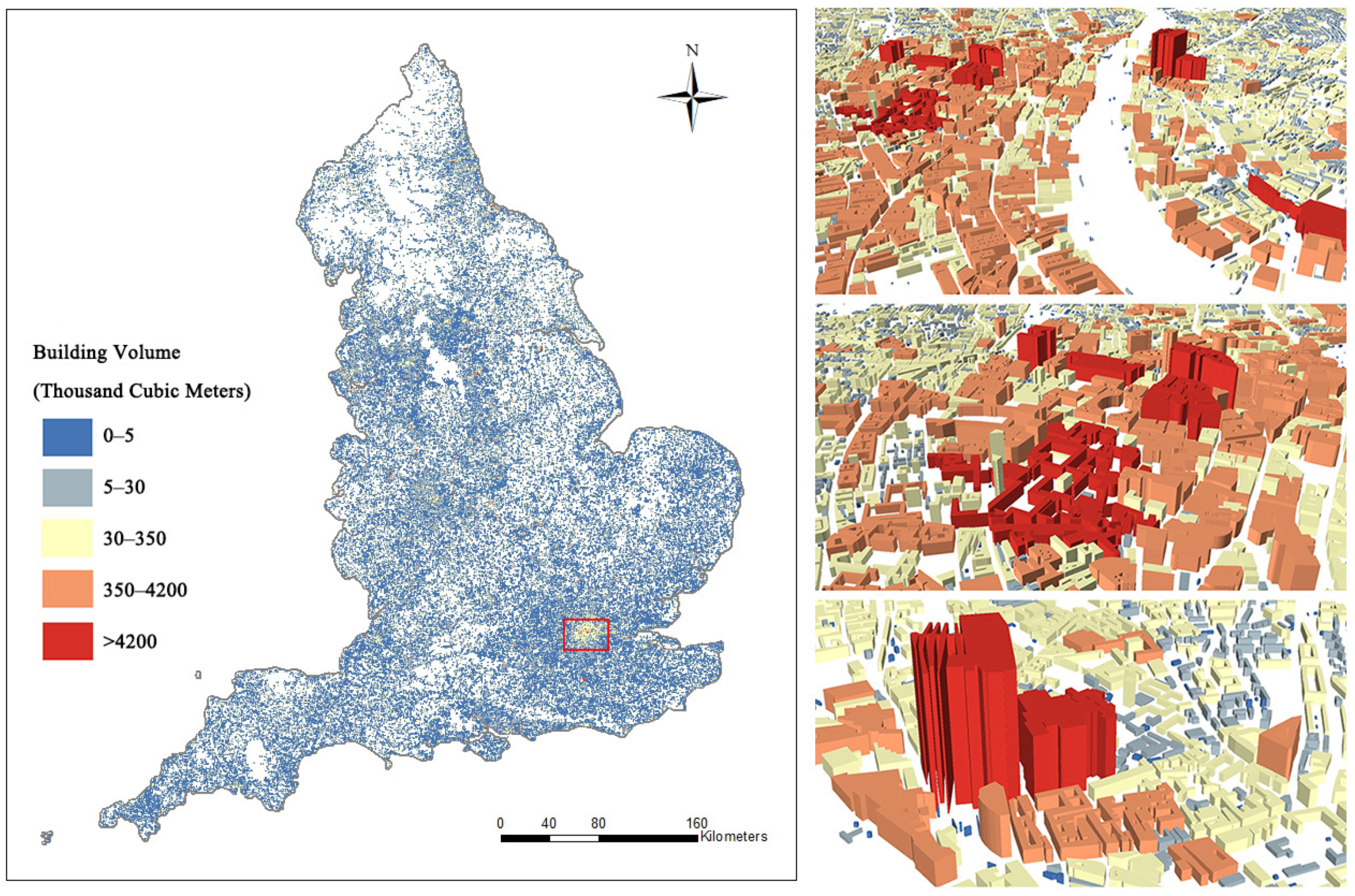
2.3.2. Building Data
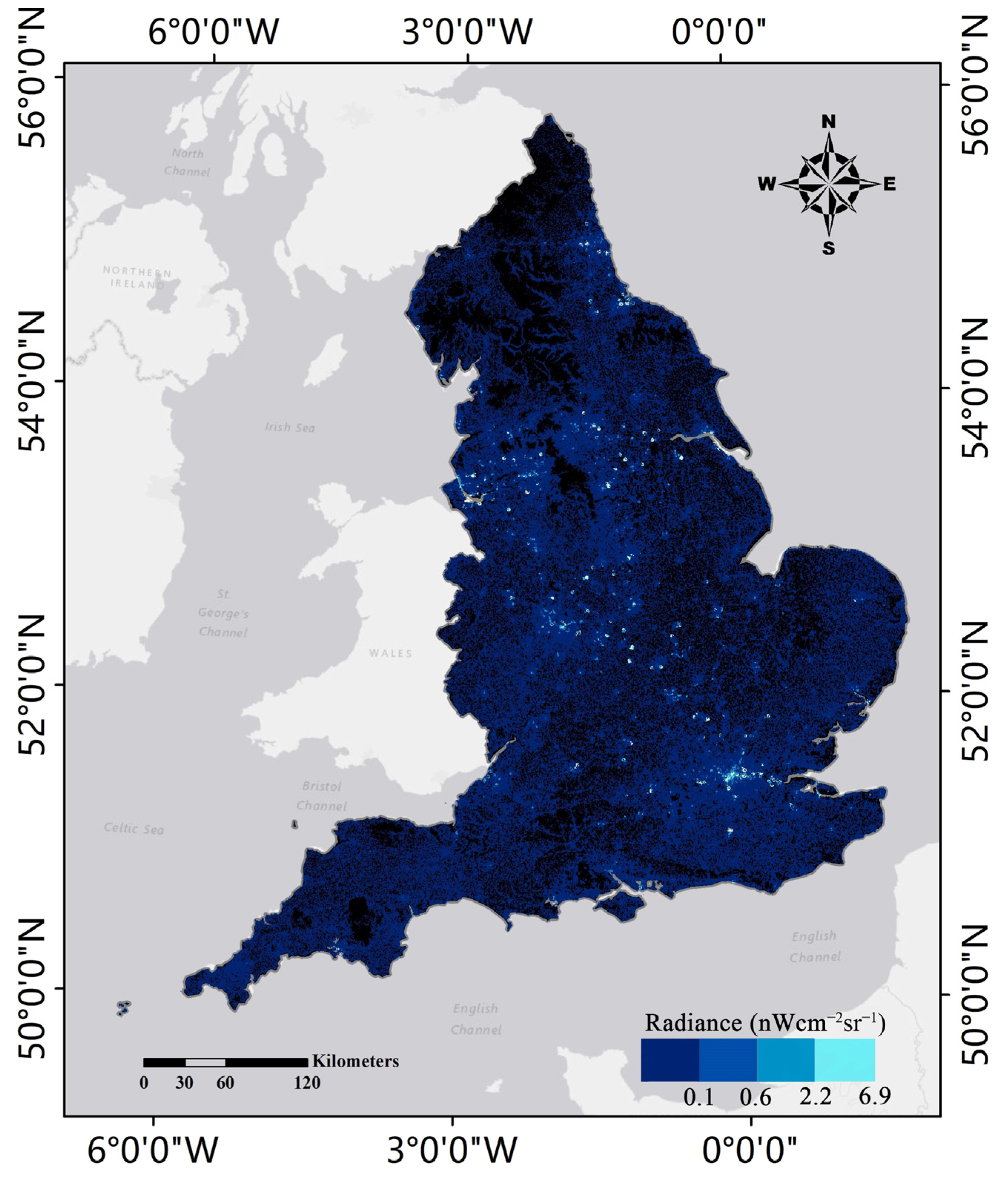
2.3.3. NPP-VIIRS Night-time Lights Imagery
2.4. Linear Regression Analysis
2.5. Evaluation Analysis
2.6. Multicollinearity Diagnosis
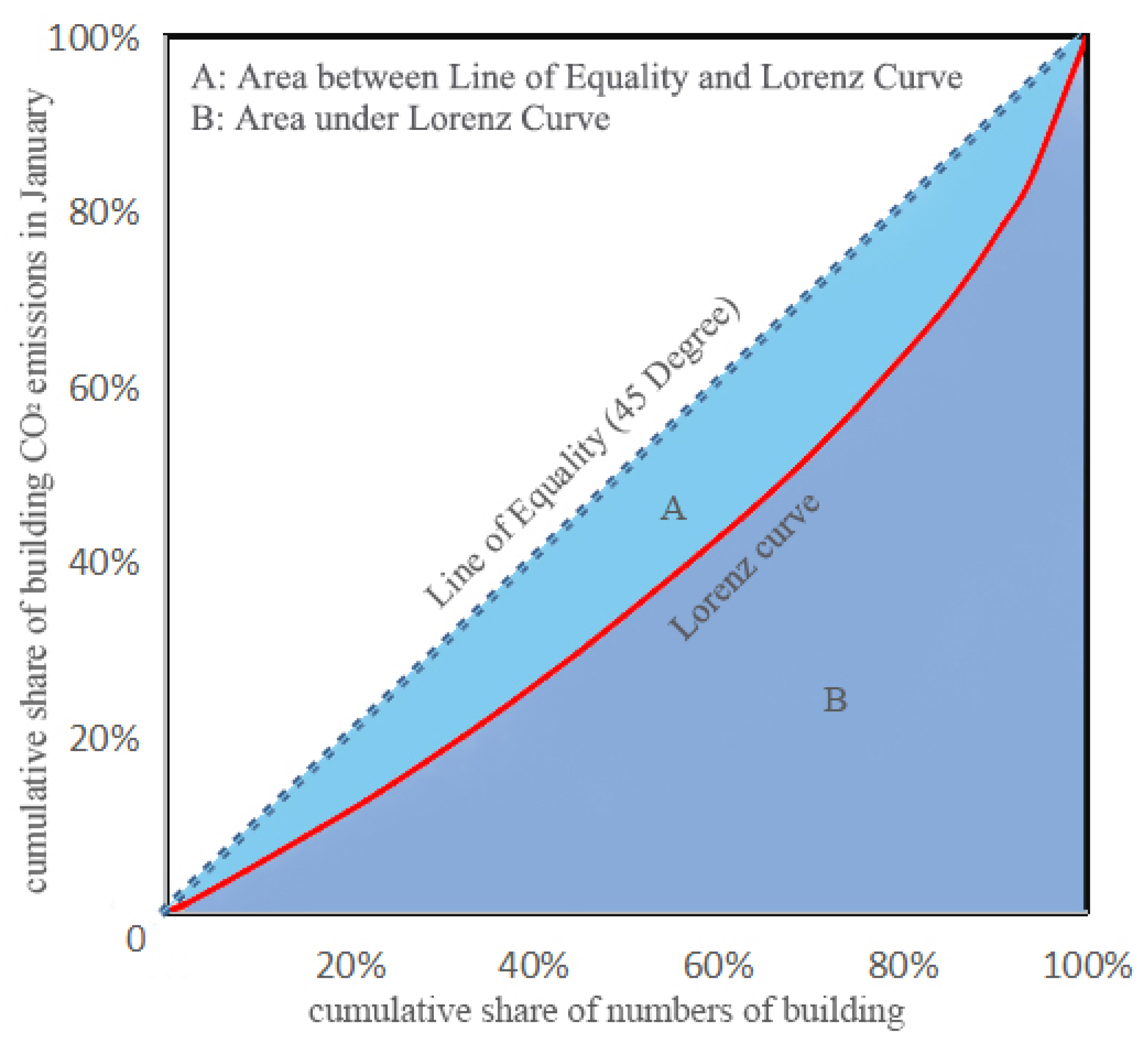
2.7. Lorenz Curve and GINI Coefficient
3. Results and Discussion
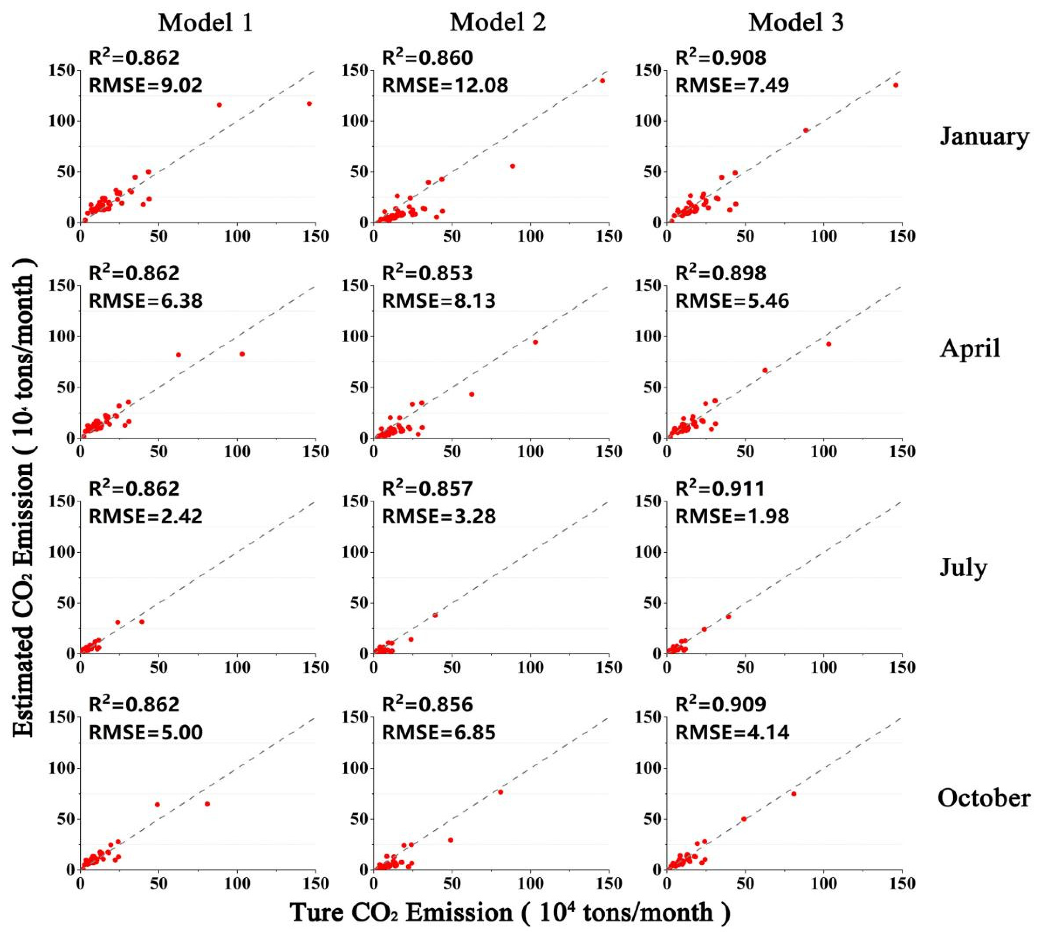
3.1. Comparison of Model Performance
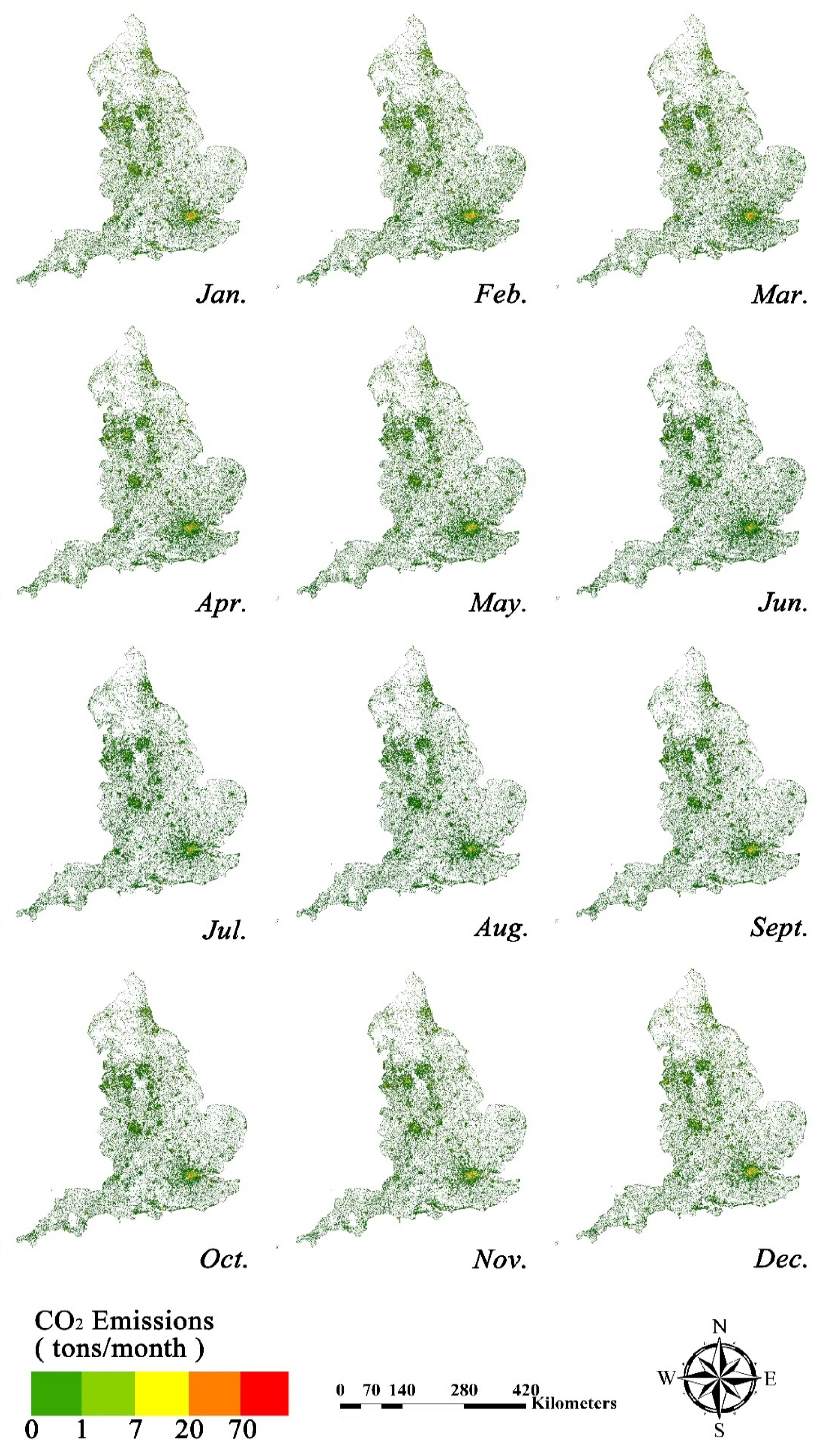
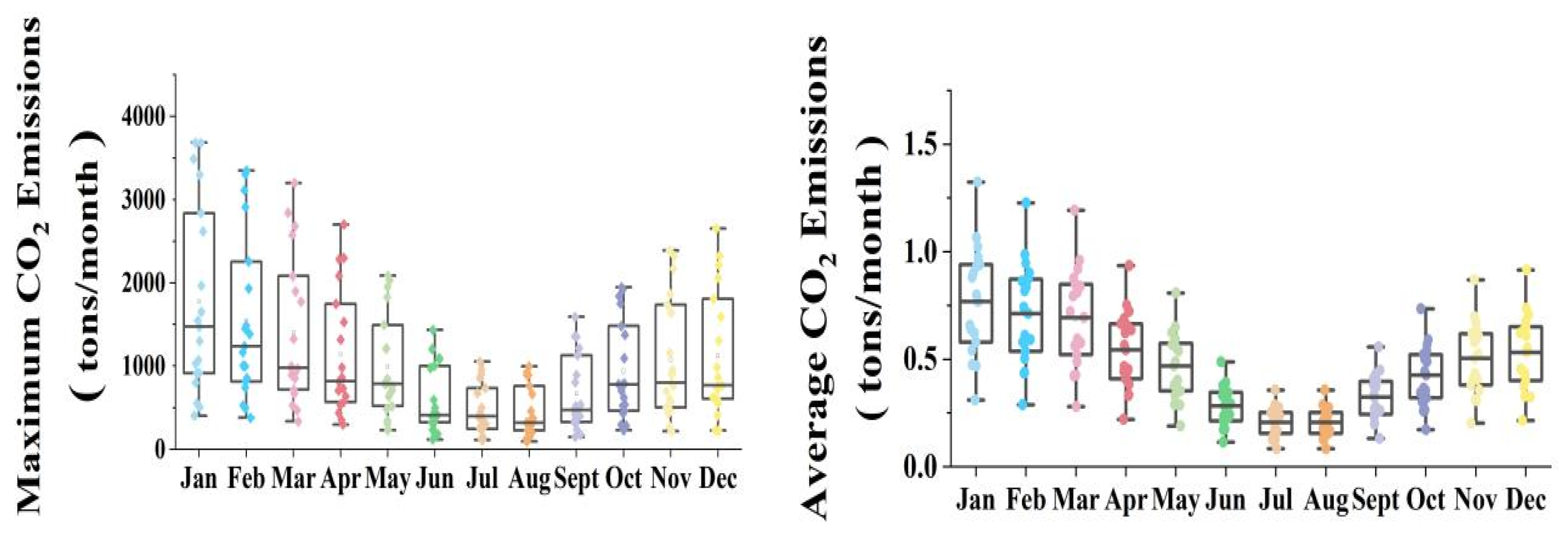
3.2. National-Scale CO2 Emissions Analysis
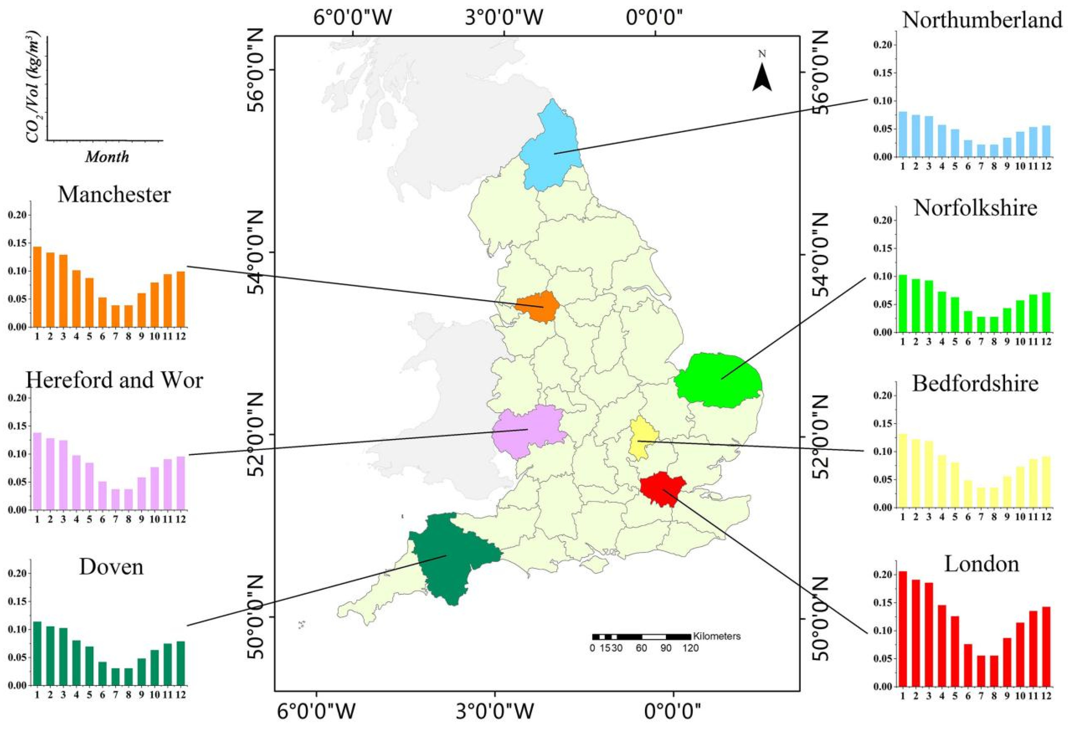
3.3. County-Scale CO2 Emissions Analysis
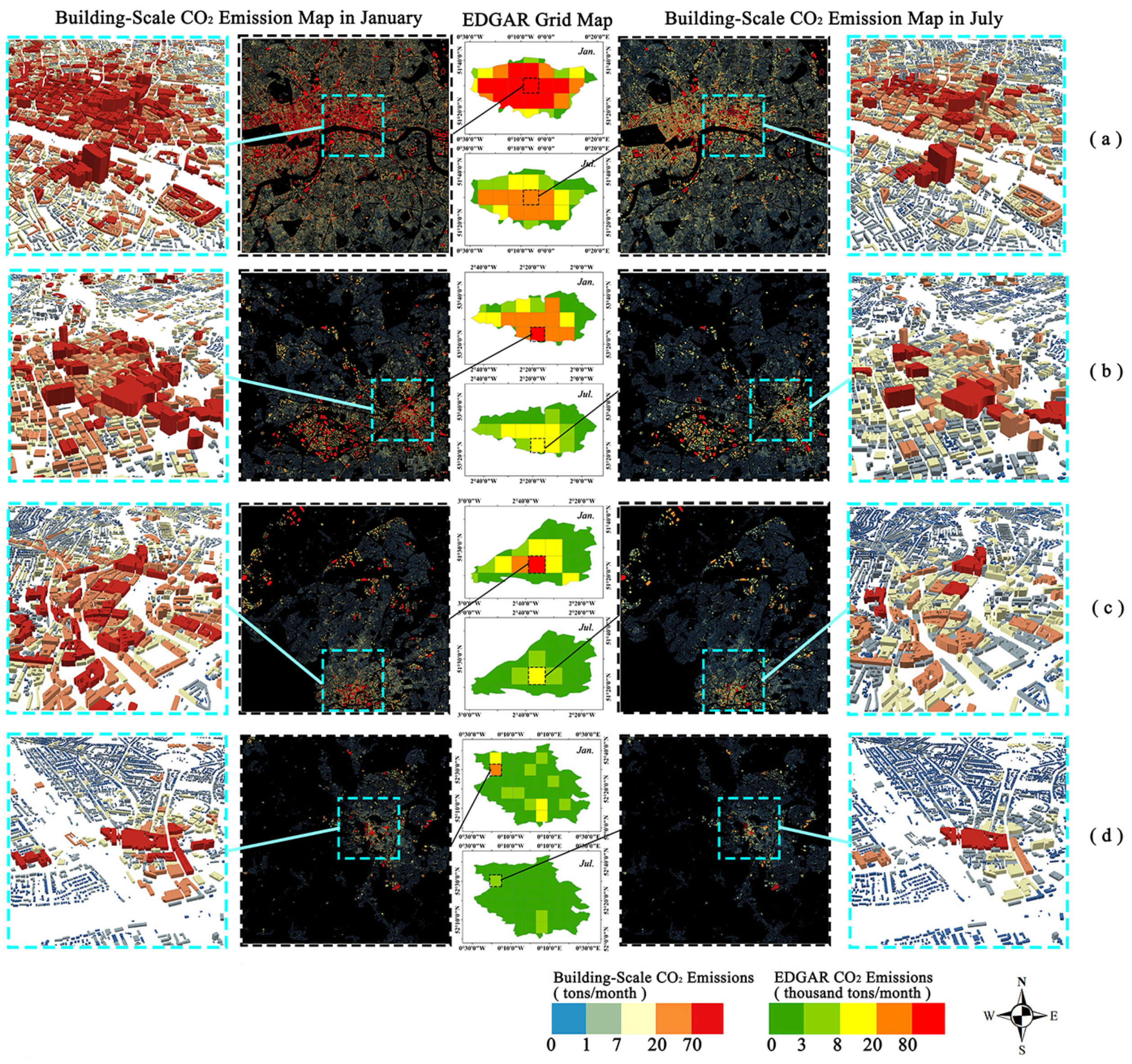
3.4. Building-Scale CO2 Emissions Analysis of Typical City
3.5. Policy Implications for CO2 Reduction
3.6. Limitations
4. Conclusions
Author Contributions
Funding
Institutional Review Board Statement
Informed Consent Statement
Data Availability Statement
Conflicts of Interest
References
- Chu, X.; Deng, X.; Jin, G.; Wang, Z.; Li, Z. Ecological security assessment based on ecological footprint approach in Beijing-Tianjin-Hebei region, China. Phys. Chem. Earth 2017, 101, 43–51. [Google Scholar] [CrossRef]
- Pata, U.K. Renewable energy consumption, urbanization, financial development, income and CO2 emissions in Turkey: Testing EKC hypothesis with structural breaks. J. Clean. Prod. 2018, 187, 770–779. [Google Scholar] [CrossRef]
- Ali, G. Climate change and associated spatial heterogeneity of Pakistan: Empirical evidence using multidisciplinary approach. Sci. Total Environ. 2018, 634, 95–108. [Google Scholar] [CrossRef] [PubMed]
- Caineng, Z.; Bo, X.; Huaqing, X.; Dewen, Z.; Zhixin, G.; Ying, W.; Luyang, J.; Songqi, P.; Songtao, W.; Batran, M. The role of new energy in carbon neutral. Pet. Explor. Dev. 2021, 48, 411–420. [Google Scholar]
- IPCC Climate Change. Mitigation of climate change. In Contribution of Working Group III to the Fifth Assessment Report of the Intergovernmental Panel on Climate Change; 2014; Volume 1454, p. 147. Available online: https://keneamazon.net/Documents/Publications/Virtual-Library/Impacto/157.pdf (accessed on 10 December 2021).
- UN Environmental Program, Environment And International Agency. Towards a zero-emission, efficient, and resilient buildings and construction sector. In Global Status Report 2017; 2017; Available online: https://www.worldgbc.org/sites/default/files/UNEP%20188_GABC_en%20%28web%29.pdf (accessed on 10 December 2021).
- File, M. Commercial Buildings Energy Consumption Survey (CBECS); US Department of Energy: Washington, DC, USA, 2015. [Google Scholar]
- Vittorini, D.; Cipollone, R. Energy saving potential in existing industrial compressors. Energy 2016, 102, 502–515. [Google Scholar] [CrossRef]
- Environment Bureau of Hong Kong. Energy and Carbon Efficiency in Buildings and Infrastructure. 2017. Available online: https://www.climateready.gov.hk/files/report/en/5.pdf (accessed on 10 December 2021).
- Seto, K.C.; Dhakal, S.; Bigio, A.; Blanco, H.; Delgado, G.C.; Dewar, D.; Huang, L.; Inaba, A.; Kansal, A.; Lwasa, S. Human settlements, infrastructure and spatial planning. In Climate Change 2014: Mitigation of Climate Change. IPCC Working Group III Contribution to AR5; Cambridge University Press: Cambridge, UK, 2014. [Google Scholar]
- Huo, T.; Ren, H.; Zhang, X.; Cai, W.; Feng, W.; Zhou, N.; Wang, X. China’s energy consumption in the building sector: A Statistical Yearbook-Energy Balance Sheet based splitting method. J. Clean. Prod. 2018, 185, 665–679. [Google Scholar] [CrossRef]
- Yan, D.; Xie, X.; Song, F.; Jiang, Y. Building environment design simulation software DeST(1): An overview of developments and information of building simulation and DeST. Heat. Vent. Air Cond. 2004, 34, 48–56. [Google Scholar]
- DeST Development Group; Tsinghua University. Simulation Analysis Method of Building Environment System: DeST; China Construction Industry Press: Beijing, China, 2006. [Google Scholar]
- Zafaranchi, M. Simulation and Analysis of Passive Parameters of Building in eQuest: A Case Study in Istanbul, Turkey. Int. J. Energy Environ. Eng. 2020, 14, 253–259. [Google Scholar]
- Luo, X.; Hong, T.; Tang, Y. Modeling thermal interactions between buildings in an urban context. Energies 2020, 13, 2382. [Google Scholar] [CrossRef]
- Robinson, D.; Haldi, F.; Leroux, P.; Perez, D.; Rasheed, A.; Wilke, U. CitySim: Comprehensive micro-simulation of resource flows for sustainable urban planning. In Proceedings of the Eleventh International IBPSA Conference, Glasgow, UK, 27–30 July 2009; pp. 1083–1090. [Google Scholar]
- Gurney, K.R.; Razlivanov, I.; Song, Y.; Zhou, Y.; Benes, B.; Abdul-Massih, M. Quantification of fossil fuel CO2 emissions on the building/street scale for a large US city. Environ. Sci. Technol. 2012, 46, 12194–12202. [Google Scholar] [CrossRef]
- Andres, R.J.; Marland, G.; Boden, T.; Bischof, S. Carbon Dioxide Emissions from Fossil Fuel Consumption and Cement Manufacture, 1751–1991; and an Estimate of Their Isotopic Composition and Latitudinal Distribution. In Proceedings of the Snowmass Global Change Institute Conference on the Global Carbon Cycle, Snowmass, CO, USA, 19–30 July 1993; Oak Ridge National Lab.: Oak Ridge, TN, USA; Oak Ridge Inst. for Science and Education: Oak Ridge, TN, USA, 1994. [Google Scholar]
- Oda, T.; Maksyutov, S. In A high-resolution global inventory of fossil fuel CO2 emission derived using a global power plant database and satellite-observed nightlight data. EGU Gen. Assem. Conf. Abstr. 2010, 12, 6550. [Google Scholar]
- Liu, Z.; Ciais, P.; Deng, Z.; Lei, R.; Davis, S.J.; Feng, S.; Zheng, B.; Cui, D.; Dou, X.; Zhu, B. Near-real-time monitoring of global CO2 emissions reveals the effects of the COVID-19 pandemic. Nat. Commun. 2020, 11, 5172. [Google Scholar] [CrossRef] [PubMed]
- Zhao, Z.; Yang, X.; Yan, H.; Huang, Y.; Zhang, G.; Lin, T.; Ye, H. Downscaling Building Energy Consumption Carbon Emissions by Machine Learning. Remote Sens. 2021, 13, 4346. [Google Scholar] [CrossRef]
- Crippa, M.; Solazzo, E.; Huang, G.; Guizzardi, D.; Koffi, E.; Muntean, M.; Schieberle, C.; Friedrich, R.; Janssens-Maenhout, G. High resolution temporal profiles in the Emissions Database for Global Atmospheric Research. Sci. Data 2020, 7, 121. [Google Scholar] [CrossRef]
- Wang, X.; Lei, Y.; Yan, L.; Liu, T.; Zhang, Q.; He, K. A unit-based emission inventory of SO2, NOx and PM for the Chinese iron and steel industry from 2010 to 2015. Sci. Total Environ. 2019, 676, 18–30. [Google Scholar] [CrossRef]
- Tong, D.; Zhang, Q.; Davis, S.J.; Liu, F.; Zheng, B.; Geng, G.; Xue, T.; Li, M.; Hong, C.; Lu, Z. Targeted emission reductions from global super-polluting power plant units. Nat. Sustain. 2018, 1, 59–68. [Google Scholar] [CrossRef] [Green Version]
- Liu, J.; Tong, D.; Zheng, Y.; Cheng, J.; Qin, X.; Shi, Q.; Yan, L.; Lei, Y.; Zhang, Q. Carbon and air pollutant emissions from China’s cement industry 1990–2015: Trends, evolution of technologies, and drivers. Atmos. Chem. Phys. 2021, 21, 1627–1647. [Google Scholar] [CrossRef]
- Dou, X.; Wang, Y.; Ciais, P.; Chevallier, F.; Davis, S.J.; Crippa, M.; Janssens-Maenhout, G.; Guizzardi, D.; Solazzo, E.; Yan, F. Near-real-time global gridded daily CO2 emissions. Innovation 2022, 3, 100182. [Google Scholar] [CrossRef]
- Chen, J.M. Carbon neutrality: Toward a sustainable future. Innovation 2021, 2, 100127. [Google Scholar] [CrossRef]
- Wang, F.; Harindintwali, J.D.; Yuan, Z.; Wang, M.; Wang, F.; Li, S.; Yin, Z.; Huang, L.; Fu, Y.; Li, L. Technologies and perspectives for achieving carbon neutrality. Innovation 2021, 2, 100180. [Google Scholar] [CrossRef]
- Shuang, Q. The Research on British Urbanization; Jilin University: Changchun, China, 2014. [Google Scholar]
- Lowes, R.; Woodman, B.; Fitch-Roy, O. Policy change, power and the development of Great Britain’s Renewable Heat Incentive. Energy Policy 2019, 131, 410–421. [Google Scholar] [CrossRef]
- Muntean, M.; Guizzardi, D.; Schaaf, E.; Crippa, M.; Solazzo, E.; Olivier, J.; Vignati, E. Fossil CO2 Emissions of All World Countries; Publications Office of the European Union: Luxembourg, 2018; Volume 2. [Google Scholar]
- Janssens-Maenhout, G.; Crippa, M.; Guizzardi, D.; Dentener, F.; Muntean, M.; Pouliot, G.; Keating, T.; Zhang, Q.; Kurokawa, J.; Wankmüller, R. HTAP_v2. 2: A mosaic of regional and global emission grid maps for 2008 and 2010 to study hemispheric transport of air pollution. Atmos. Chem. Phys. 2015, 15, 11411–11432. [Google Scholar] [CrossRef] [Green Version]
- Crippa, M.; Oreggioni, G.; Guizzardi, D.; Muntean, M.; Schaaf, E.; Lo Vullo, E.; Solazzo, E.; Monforti-Ferrario, F.; Olivier, J.; Vignati, E.E. EDGAR v5.0 Greenhouse Gas Emissions; European Commission, Joint Research Centre (JRC) [National CO2 Emissions Per Sector and Gridmaps of Total CO2 Emissions]. 2019. Available online: https://publications.jrc.ec.europa.eu/repository/handle/JRC122515 (accessed on 10 December 2021).
- Qin, J.; Fang, C.; Wang, Y.; Li, G.; Wang, S. Evaluation of three-dimensional urban expansion: A case study of Yangzhou City, Jiangsu Province, China. Chin. Geogr. Sci. 2015, 25, 224–236. [Google Scholar] [CrossRef]
- Chen, Y.; Li, X.; Zheng, Y.; Guan, Y.; Liu, X. Estimating the relationship between urban forms and energy consumption: A case study in the Pearl River Delta, 2005–2008. Landsc. Urban Planing 2011, 102, 33–42. [Google Scholar] [CrossRef]
- Liu, M.; Hu, Y.; Li, C. Landscape metrics for three-dimensional urban building pattern recognition. Appl. Geogr. 2017, 87, 66–72. [Google Scholar] [CrossRef]
- Xu, X.; Ou, J.; Liu, P.; Liu, X.; Zhang, H. Investigating the impacts of three-dimensional spatial structures on CO2 emissions at the urban scale. Sci. Total Environ. 2021, 762, 143096. [Google Scholar] [CrossRef]
- Li, X.; Zhou, W. Dasymetric mapping of urban population in China based on radiance corrected DMSP-OLS nighttime light and land cover data. Sci. Total Environ. 2018, 643, 1248–1256. [Google Scholar] [CrossRef]
- Bennett, M.M.; Smith, L.C. Advances in using multitemporal night-time lights satellite imagery to detect, estimate, and monitor socioeconomic dynamics. Remote Sens. Environ. 2017, 192, 176–197. [Google Scholar] [CrossRef]
- Small, C.; Pozzi, F.; Elvidge, C.D. Spatial analysis of global urban extent from DMSP-OLS night lights. Remote Sens. Environ. 2005, 96, 277–291. [Google Scholar] [CrossRef]
- Lv, Q.; Liu, H.; Wang, J.; Liu, H.; Shang, Y. Multiscale analysis on spatiotemporal dynamics of energy consumption CO2 emissions in China: Utilizing the integrated of DMSP-OLS and NPP-VIIRS nighttime light datasets. Sci. Total Environ. 2020, 703, 134394. [Google Scholar] [CrossRef]
- Zhang, W.; Cui, Y.; Wang, J.; Wang, C.; Streets, D.G. How does urbanization affect CO2 emissions of central heating systems in China? An assessment of natural gas transition policy based on nighttime light data. J. Clean. Prod. 2020, 276, 123188. [Google Scholar] [CrossRef]
- Elvidge, C.D.; Baugh, K.E.; Zhizhin, M.; Hsu, F. Why VIIRS data are superior to DMSP for mapping nighttime lights. Proc. Asia-Pac. Adv. Netw. 2013, 35, 62. [Google Scholar] [CrossRef] [Green Version]
- Ou, J.; Liu, X.; Li, X.; Li, M.; Li, W. Evaluation of NPP-VIIRS nighttime light data for mapping global fossil fuel combustion CO2 emissions: A comparison with DMSP-OLS nighttime light data. PLoS ONE 2015, 10, e138310. [Google Scholar] [CrossRef] [PubMed] [Green Version]
- Ray, J.; Yadav, V.; Michalak, A.M.; van Bloemen Waanders, B.; McKenna, S.A. A multiresolution spatial parameterization for the estimation of fossil-fuel carbon dioxide emissions via atmospheric inversions. Geosci. Model. Dev. 2014, 7, 1901–1918. [Google Scholar] [CrossRef] [Green Version]
- Wang, R.; Tao, S.; Ciais, P.; Shen, H.Z.; Huang, Y.; Chen, H.; Shen, G.F.; Wang, B.; Li, W.; Zhang, Y.Y. High-resolution mapping of combustion processes and implications for CO2 emissions. Atmos. Chem. Phys. 2013, 13, 5189–5203. [Google Scholar] [CrossRef] [Green Version]
- Cui, Y.; Zhang, W.; Wang, C.; Streets, D.G.; Xu, Y.; Du, M.; Lin, J. Spatiotemporal dynamics of CO2 emissions from central heating supply in the North China Plain over 2012–2016 due to natural gas usage. Appl. Energy 2019, 241, 245–256. [Google Scholar] [CrossRef]
- Hosseini, S.M.; Saifoddin, A.; Shirmohammadi, R.; Aslani, A. Forecasting of CO2 emissions in Iran based on time series and regression analysis. Energy Rep. 2019, 5, 619–631. [Google Scholar] [CrossRef]
- Asumadu-Sarkodie, S.; Owusu, P.A. Recent evidence of the relationship between carbon dioxide emissions, energy use, GDP, and population in Ghana: A linear regression approach. Energy Sources Part B Econ. Plan. Policy 2017, 12, 495–503. [Google Scholar] [CrossRef]
- Wang, S.; Liu, X. China’s city-level energy-related CO2 emissions: Spatiotemporal patterns and driving forces. Appl. Energy 2017, 200, 204–214. [Google Scholar] [CrossRef]
- Chen, Y.; Tan, H.; Berardi, U. A data-driven approach for building energy benchmarking using the Lorenz curve. Energy Build. 2018, 169, 319–331. [Google Scholar] [CrossRef]
- Milanovic, B. A simple way to calculate the Gini coefficient, and some implications. Econ. Lett. 1997, 56, 45–49. [Google Scholar] [CrossRef]
- Kong, Y.; Zhao, T.; Yuan, R.; Chen, C. Allocation of carbon emission quotas in Chinese provinces based on equality and efficiency principles. J. Clean. Prod. 2019, 211, 222–232. [Google Scholar] [CrossRef]
- Hidalgo, J.C.G.; Angulo, D.P.; Portugués, S.B. Temporal variations of trends in the Central England Temperature series. Cuad. Investig. Geográfica/Geogr. Res. Lett. 2020, 46, 345–369. [Google Scholar] [CrossRef] [Green Version]
- Xiao, W.; Qin, D.; Li, W.; Chu, J. Model for distribution of water pollutants in a lake basin based on environmental Gini coefficient. Acta Sci. Circumstantiae 2009, 29, 1765–1771. [Google Scholar]
- Gowrishankar, V.; Levin, A. America’s Clean Energy Frontier: The Pathway to a Safer Climate Future; Resource Defense Council Report; New York, NY, USA, 2017; p. 16. Available online: https://www.ourenergypolicy.org/wp-content/uploads/2017/09/americas-clean-energy-frontier-report.pdf (accessed on 10 December 2021).

| Month | Model 1 | Model 2 | Model 3 | |||||||||
|---|---|---|---|---|---|---|---|---|---|---|---|---|
| R2 | Adjusted R2 | MRE(%) | RMSE (104 tons) | R2 | Adjusted R2 | MRE(%) | RMSE (104 tons) | R2 | Adjusted R2 | MRE(%) | RMSE (104 tons) | |
| January | 0.862 | 0.859 | 34.02 | 9.02 | 0.860 | 0.856 | 48.67 | 12.08 | 0.908 | 0.904 | 24.86 | 7.49 |
| February | 0.862 | 0.859 | 34.02 | 8.36 | 0.854 | 0.851 | 48.86 | 11.05 | 0.906 | 0.901 | 25.38 | 6.93 |
| March | 0.862 | 0.859 | 34.04 | 8.13 | 0.858 | 0.855 | 46.80 | 10.45 | 0.902 | 0.897 | 24.70 | 6.89 |
| April | 0.862 | 0.859 | 34.04 | 6.38 | 0.853 | 0.849 | 47.00 | 8.13 | 0.898 | 0.893 | 25.58 | 5.46 |
| May | 0.862 | 0.859 | 34.06 | 5.51 | 0.858 | 0.855 | 46.62 | 7.16 | 0.904 | 0.900 | 24.85 | 4.62 |
| June | 0.862 | 0.859 | 34.01 | 3.32 | 0.873 | 0.870 | 49.64 | 4.03 | 0.897 | 0.892 | 25.34 | 2.93 |
| July | 0.862 | 0.859 | 34.03 | 2.42 | 0.857 | 0.853 | 49.03 | 3.28 | 0.911 | 0.906 | 24.38 | 1.98 |
| August | 0.862 | 0.859 | 34.03 | 2.42 | 0.859 | 0.856 | 49.83 | 3.20 | 0.903 | 0.898 | 25.55 | 2.06 |
| September | 0.862 | 0.859 | 34.05 | 3.80 | 0.871 | 0.874 | 49.16 | 4.90 | 0.910 | 0.905 | 24.54 | 3.20 |
| October | 0.862 | 0.859 | 34.01 | 5.00 | 0.856 | 0.852 | 50.34 | 6.85 | 0.909 | 0.904 | 24.09 | 4.14 |
| November | 0.862 | 0.859 | 34.00 | 5.91 | 0.855 | 0.852 | 50.21 | 7.98 | 0.905 | 0.901 | 24.99 | 4.96 |
| December | 0.862 | 0.859 | 34.02 | 6.24 | 0.844 | 0.841 | 48.40 | 8.15 | 0.892 | 0.886 | 26.02 | 5.48 |
| Month | Building Data | Nightlight Data | F | Sig. | ||||
|---|---|---|---|---|---|---|---|---|
| ai | Sig. | VIF | bi | Sig. | VIF | |||
| January | 88.19 | 0.000 | 5.059 | 51.05 | 0.000 | 5.059 | 202.961 | 0.000 |
| February | 83.99 | 0.000 | 5.003 | 46.37 | 0.000 | 5.003 | 197.720 | 0.000 |
| March | 79.79 | 0.000 | 5.674 | 44.12 | 0.000 | 5.674 | 188.289 | 0.000 |
| April | 64.44 | 0.000 | 5.784 | 32.86 | 0.001 | 5.784 | 180.626 | 0.000 |
| May | 54.02 | 0.000 | 5.388 | 29.78 | 0.000 | 5.388 | 193.823 | 0.000 |
| June | 28.62 | 0.000 | 7.912 | 18.83 | 0.001 | 7.912 | 178.664 | 0.000 |
| July | 24.10 | 0.000 | 4.722 | 14.72 | 0.000 | 4.722 | 208.689 | 0.000 |
| August | 23.64 | 0.000 | 5.606 | 14.03 | 0.000 | 5.606 | 190.948 | 0.000 |
| September | 33.92 | 0.000 | 5.772 | 23.01 | 0.000 | 5.772 | 206.266 | 0.000 |
| October | 49.90 | 0.000 | 4.832 | 28.34 | 0.000 | 4.832 | 204.037 | 0.000 |
| November | 59.08 | 0.000 | 5.126 | 36.12 | 0.000 | 5.126 | 196.197 | 0.000 |
| December | 66.29 | 0.000 | 6.107 | 37.53 | 0.002 | 6.107 | 168.848 | 0.000 |
| Month | Max CO2 (tons) | Ave CO2 (tons) | CO2/Vol (kg/m3) |
|---|---|---|---|
| January | 3682 | 0.830 | 0.152 |
| February | 3348 | 0.770 | 0.141 |
| March | 2575 | 0.748 | 0.137 |
| April | 2300 | 0.587 | 0.108 |
| May | 2087 | 0.507 | 0.093 |
| June | 978 | 0.306 | 0.056 |
| July | 960 | 0.223 | 0.041 |
| August | 894 | 0.223 | 0.041 |
| September | 1215 | 0.350 | 0.064 |
| October | 1840 | 0.460 | 0.084 |
| November | 2389 | 0.545 | 0.100 |
| December | 2216 | 0.574 | 0.105 |
Publisher’s Note: MDPI stays neutral with regard to jurisdictional claims in published maps and institutional affiliations. |
© 2022 by the authors. Licensee MDPI, Basel, Switzerland. This article is an open access article distributed under the terms and conditions of the Creative Commons Attribution (CC BY) license (https://creativecommons.org/licenses/by/4.0/).
Share and Cite
Zheng, Y.; Ou, J.; Chen, G.; Wu, X.; Liu, X. Mapping Building-Based Spatiotemporal Distributions of Carbon Dioxide Emission: A Case Study in England. Int. J. Environ. Res. Public Health 2022, 19, 5986. https://doi.org/10.3390/ijerph19105986
Zheng Y, Ou J, Chen G, Wu X, Liu X. Mapping Building-Based Spatiotemporal Distributions of Carbon Dioxide Emission: A Case Study in England. International Journal of Environmental Research and Public Health. 2022; 19(10):5986. https://doi.org/10.3390/ijerph19105986
Chicago/Turabian StyleZheng, Yue, Jinpei Ou, Guangzhao Chen, Xinxin Wu, and Xiaoping Liu. 2022. "Mapping Building-Based Spatiotemporal Distributions of Carbon Dioxide Emission: A Case Study in England" International Journal of Environmental Research and Public Health 19, no. 10: 5986. https://doi.org/10.3390/ijerph19105986
APA StyleZheng, Y., Ou, J., Chen, G., Wu, X., & Liu, X. (2022). Mapping Building-Based Spatiotemporal Distributions of Carbon Dioxide Emission: A Case Study in England. International Journal of Environmental Research and Public Health, 19(10), 5986. https://doi.org/10.3390/ijerph19105986