
Heterogeneous Effects of Health Insurance on Rural Children’s Health in China: A Causal Machine Learning Approach

Abstract
:1. Introduction
2. Background
2.1. The Urban and Rural Resident Basic Medical Insurance (URRBMI)
2.2. Literature Review
3. Data and Descriptive Statistics
3.1. Data and Variables
3.2. Descriptive Statistics
4. Empirical Framework
4.1. Theoretical Basis
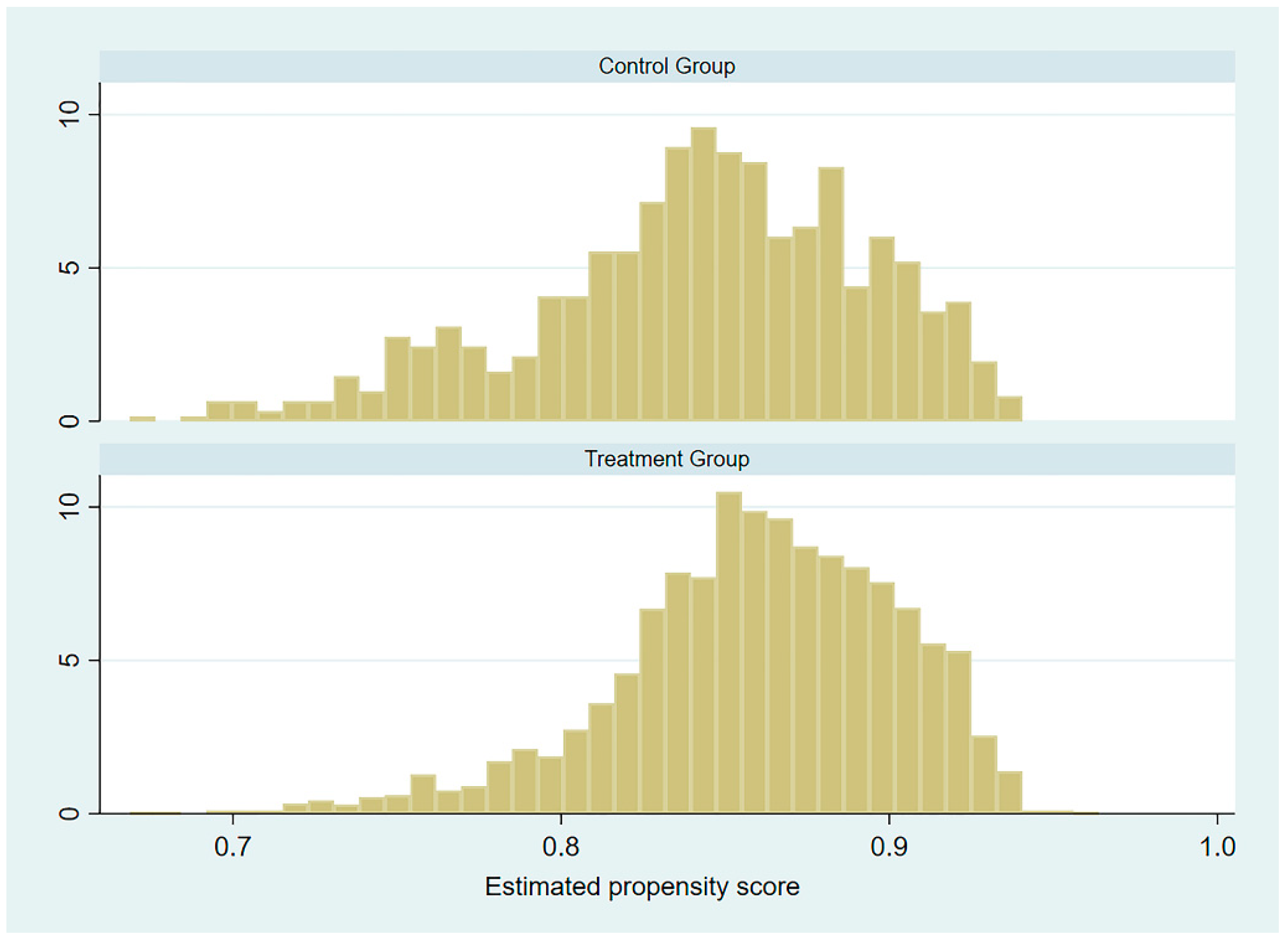
4.2. Propensity Score Matching (PSM)
4.3. Causal Forest
5. Results
5.1. The Average Treatment Effect
5.2. Heterogeneity Analysis
6. Conclusions
Author Contributions
Funding
Institutional Review Board Statement
Informed Consent Statement
Data Availability Statement
Conflicts of Interest
References
- Lei, X.; Lin, W. The new cooperative medical scheme in rural China: Does more coverage mean more service and better health? Health Econ. 2009, 18, S25–S46. [Google Scholar] [CrossRef]
- Cheng, L.; Liu, H.; Zhang, Y.; Shen, K.; Zeng, Y. The impact of health insurance on health out-comes and spending of the elderly: Evidence from China’s New Cooperative Medical Scheme. Health Econ. 2015, 24, 672–691. [Google Scholar] [CrossRef]
- Sun, Y. Welfare consequences of access to health insurance for rural households: Evidence from the New Cooperative Medical Scheme in China. Health Econ. 2019, 29, 337–352. [Google Scholar] [CrossRef]
- Shao, H.K.; Sheng, J. The effect of national health insurance on mortality and the SES—Health gradient: Evidence from the elderly in Taiwan. Health Econ. 2013, 22, 52–72. [Google Scholar] [CrossRef]
- Petticrew, M.; Tugwell, P.; Kristjansson, E.; Oliver, S.; Ueffing, E.; Welch, V. Damned if you do, damned if you don’t: Subgroup analysis and equity. J. Epidemiol. Community Health 2011, 66, 95–98. [Google Scholar] [CrossRef]
- Hainmueller, J.; Mummolo, J.; Xu, Y. How much should we trust estimates from multiplicative interaction models? Simple tools to improve empirical practice. Political Anal. 2019, 27, 163–192. [Google Scholar] [CrossRef] [Green Version]
- Athey, S.; Imbens, G. Recursive partitioning for heterogeneous causal effects. Proc. Natl. Acad. Sci. USA 2016, 113, 7353–7360. [Google Scholar] [CrossRef] [Green Version]
- Hanratty, M. Canadian national health insurance and infant health. Am. Econ. Rev. 1996, 86, 276–284. Available online: https://www.jstor.org/stable/2118267 (accessed on 12 September 2021).
- Currie, J.; Gruber, J. Health insurance eligibility, utilization of medical care and child health. Q. J. Econ. 1996, 111, 431–466. [Google Scholar] [CrossRef] [Green Version]
- Currie, J.; Gruber, J. Saving babies: The efficacy and cost of recent changes in the Medicaid eligibility of pregnant women. J. Political Econ. 1996, 104, 1263–1296. [Google Scholar] [CrossRef]
- Currie, J.; Gruber, J. The technology of birth: Health insurance, medical interventions and infant health. In Working Paper 5985; National Bureau Economic Research: Cambridge, MA, USA, 1997. [Google Scholar] [CrossRef]
- Currie, J.; Decker, S.; Lin, W. Has public health insurance for older children reduced disparities in access to care and health outcomes? J. Health Econ. 2008, 27, 1567–1581. [Google Scholar] [CrossRef]
- Wagstaff, A.; Pradhan, M. Health insurance impacts on health and nonmedical consumption in a developing country. In World Bank Policy Research Working Paper; World Bank: Washington, DC, USA, 2005; Number 3563. [Google Scholar]
- Chou, S.Y.; Grossman, M.; Liu, J.T. The impact of national health insurance on birth outcomes: A natural experiment in Taiwan. J. Dev. Econ. 2014, 111, 75–91. [Google Scholar] [CrossRef]
- Chen, Y.; Jin, G.Z. Does health insurance coverage lead to better health and educational out-comes? Evidence from rural China. J. Health Econ. 2012, 31, 1–14. [Google Scholar] [CrossRef] [Green Version]
- Alcaraz, C.; Chiquiar, D.; Orraca, M.J.; Salcedo, A. The effect of Publicly Provided Health In-surance on Education Outcomes in Mexico. World Bank Econ. Rev. 2017, 30, S145–S156. [Google Scholar] [CrossRef] [Green Version]
- Bagnoli, L. Does health insurance improve health for all? Heterogeneous effects on children in Ghana. World Dev. 2019, 124, 1–15. [Google Scholar] [CrossRef]
- Athey, S.; Imbens, G. The state of applied econometrics: Causality and policy evaluation. J. Econ. Perspect. 2017, 31, 3–32. [Google Scholar] [CrossRef] [Green Version]
- Wager, S.; Athey, S. Estimation and inference of heterogeneous treatment effects using random forests. J. Am. Stat. Assoc. 2018, 113, 1228–1242. [Google Scholar] [CrossRef] [Green Version]
- Chin, S.; Kahn, M.E.; Moon, H.R. Estimating the gains from new rail transit investment: A ma-chine learning tree approach. Real Estate Econ. 2020, 48, 886–914. [Google Scholar] [CrossRef] [Green Version]
- Andrew, J.T. Machine Learning and Causality: The Impact of Financial Crises on Growth; International Monetary Fund: Washington, DC, USA, 2019. [Google Scholar]
- Noemi, K.; Andrew, M.; Rodrigo, M.S.; Taufik, H.; Karla, D.; Marc, S. Who benefits from health insurance? Uncovering heterogeneous policy impacts using causal machine learning. In Working Paper. CHE Research Paper; Centre for Health Economics, University of York: York, UK, 2020. [Google Scholar]
- Rosenbaum, P.R.; Rubin, D.B. The central role of the propensity score in observational studies for causal effects. Biometrika 1983, 70, 41–55. [Google Scholar] [CrossRef]
- Robinson, P.M. Root-N-consistent semiparametric regression. Econom. Soc. 1988, 56, 931–954. [Google Scholar] [CrossRef] [Green Version]
- Chernozhukov, V.; Chetverikov, D.; Demirer, M.; Duflo, E.; Hansen, C.; Newey, W.; Robins, J. Double/debiased machine learning for treatment and structural parameters. Econom. J. 2018, 21, C1–C68. [Google Scholar] [CrossRef]
- Athey, S.; Tibshirani, J.; Wager, S. Generalized random forests. Ann. Stat. 2019, 47, 1148–1178. [Google Scholar] [CrossRef] [Green Version]
- Breiman, L. Random forests. Mach. Learn. 2001, 45, 5–32. [Google Scholar] [CrossRef] [Green Version]
- Meng, Q.; Chi, W.S.; Ran, T. BitCoin: A New Basket for Eggs. Econ. Model. 2020, 94, 896–907. [Google Scholar] [CrossRef]
- Su, C.W.; Qin, M.; Tao, R.; Umar, M. Financial implications of fourth industrial revolution: Can bitcoin improve prospects of energy investment? Technol. Forecast. Soc. Chang. 2020, 158, 1–8. [Google Scholar] [CrossRef]
- Tibshirani, J.; Athey, S.; Wager, S.; Friedberg, R.; Miner, L.; Wright, M. Grf: Generalized Ran-dom Forests (Beta). 2018. Available online: https://grf-labs.github.io/grf (accessed on 12 September 2021).
- Athey, S.; Wager, S. Estimating treatment effects with causal forests: An application. Obs. Stud. 2019, 5, 37–51. [Google Scholar] [CrossRef]
- Chernozhukov, V.; Demirer, M.; Duflo, E.; Fernandez-Val, I. Generic machine learning inference on heterogeneous treatment effects in randomized experiments. In Working Paper 24678; National Bureau Economic Research: Cambridge, MA, USA, 2018. [Google Scholar] [CrossRef]
- Nie, X.; Wager, S. Quasi-oracle estimation of heterogeneous treatment effects. Biometrika 2021, 108, 299–319. [Google Scholar] [CrossRef]

| Variables | Definition | Treatment Group | Control Group | Differences |
|---|---|---|---|---|
| Weight for Height Z-score (WHZ) | WHZ compares a child’s weight to the weight of a child of the same length/height and sex to classify nutritional status. | −0.185 (0.802) | −0.376 (0.770) | −0.191 *** |
| Weight for Age Z-score (WAZ) | WAZ compares a child’s weight to the weight of a child of the same age and sex to classify nutritional status. | 0.022 (1.012) | −0.091 (0.929) | −0.112 ** |
| Height by Age Z-score (HAZ) | HAZ compares a child’s height to the height of a child of the same age and sex to classify nutritional status. | 0.020 (0.991) | −0.069 (1.012) | −0.090 |
| Body Mass Index (BMI) | Weight (kg)/height2 (m2) | 18.283 (5.209) | 18.944 (6.703) | 0.661 ** |
| Child’s characteristics | ||||
| Gender | 1 if male; 0 if female | 0.539 (0.499) | 0.501 (0.500) | −0.037 * |
| Age | Age of the child | 7.813 (4.241) | 5.765 (4.807) | −2.048 *** |
| Mother’s characteristics | ||||
| Age | Age of the child’s mother | 34.211 (6.590) | 32.694 (6.895) | −1.517 *** |
| Education | 1 if no formal education; 2 if primary school; 3 if junior high school; 4 if high school; 5 if junior college; 6 if bachelor degree; 7 if master. | 2.676 (1.143) | 3.057 (1.393) | 0.381 *** |
| Family characteristics | ||||
| Household income per capita | Logarithm of household income per capita | 8.994 (0.890) | 9.079 (1.059) | 0.085 ** |
| Living area | 1 if urban area; 0 if rural area | 0.332 (0.471) | 0.455 (0.498) | 0.123 *** |
| Geographic location | 1 if eastern region; 2 if central region; 3 if western region | 2.047 (0.819) | 1.816 (0.827) | −0.232 *** |
| Dependent Variables | N | Nearest Neighbor Matching (1:1) | Nearest Neighbor Matching (1:4) | Nuclear Match |
|---|---|---|---|---|
| Weight for Height Z-score (WHZ) | 2015 | 0.199 *** (0.055) | 0.183 *** (0.046) | 0.189 *** (0.044) |
| Weight for Age Z-score (WAZ) | 2015 | 0.155 ** (0.064) | 0.158 ** (0.056) | 0.131 ** (0.053) |
| Height by Age Z-score (HAZ) | 2015 | 0.213 ** (0.072) | 0.168 ** (0.060) | 0.134 ** (0.057) |
| Body Mass Index (BMI) | 3537 | −0.799 (0.468) | −0.634 (0.396) | −0.687 (0.375) |
| Rank | Preschool Children | School-Age Children | ||
|---|---|---|---|---|
| Variable | Importance | Variable | Importance | |
| 1 | Age of the child’s mother | 0.368 | Mother’s education: no formal education | 0.263 |
| 2 | Age of the child | 0.158 | Age of the child’s mother | 0.200 |
| 3 | Mother’s education: no formal education | 0.155 | Age of the child | 0.149 |
| 4 | Mother’s education: bachelor degree | 0.060 | Wealth quantile 5 | 0.115 |
| 5 | Geographic location: central region | 0.036 | Living area: rural area | 0.099 |
| 6 | Mother’s education: primary school | 0.033 | Geographic location: central region | 0.036 |
| 7 | Child’s gender: male | 0.031 | Child’s gender: male | 0.029 |
| 8 | Wealth quantile 3 | 0.025 | Geographic location: western region | 0.026 |
| 9 | Living area: rural area | 0.022 | Mother’s education: junior college | 0.019 |
| 10 | Wealth quantile 2 | 0.021 | Wealth quantile 3 | 0.017 |
| Preschool Children | School-Age Children | ||
|---|---|---|---|
| Subgroups | CATC | Subgroups | CATC |
| Mother’s education: primary school | 0.214 ** (0.174) | Mother’s education: no formal education | −3.650 (1.290) |
| Living area: rural area | 0.118 ** (0.090) | Living area: rural area | −1.835 (0.542) |
| Living area: urban area | 0.140 (0.075) | Living area: urban area | 0.285 * (0.369) |
| Child’s gender: male | 0.098 ** (0.236) | Child’s gender: male | −1.410 (0.610) |
| Child’s gender: female | 0.139 (0.092) | Child’s gender: female | −0.423 (0.345) |
| Geographic location: central region | 0.205 (0.106) | Geographic location: western region | −2.030 (1.030) |
| Wealth quantile 2 | 0.218 * (0.152) | Wealth quantile 2 | −0.726 (0.568) |
| Wealth quantile 5 | 0.160 (0.097) | Wealth quantile 4 | −1.243 (0.519) |
Publisher’s Note: MDPI stays neutral with regard to jurisdictional claims in published maps and institutional affiliations. |
© 2021 by the authors. Licensee MDPI, Basel, Switzerland. This article is an open access article distributed under the terms and conditions of the Creative Commons Attribution (CC BY) license (https://creativecommons.org/licenses/by/4.0/).
Share and Cite
Chen, H.; Xing, J.; Yang, X.; Zhan, K. Heterogeneous Effects of Health Insurance on Rural Children’s Health in China: A Causal Machine Learning Approach. Int. J. Environ. Res. Public Health 2021, 18, 9616. https://doi.org/10.3390/ijerph18189616
Chen H, Xing J, Yang X, Zhan K. Heterogeneous Effects of Health Insurance on Rural Children’s Health in China: A Causal Machine Learning Approach. International Journal of Environmental Research and Public Health. 2021; 18(18):9616. https://doi.org/10.3390/ijerph18189616
Chicago/Turabian StyleChen, Hua, Jianing Xing, Xiaoxu Yang, and Kai Zhan. 2021. "Heterogeneous Effects of Health Insurance on Rural Children’s Health in China: A Causal Machine Learning Approach" International Journal of Environmental Research and Public Health 18, no. 18: 9616. https://doi.org/10.3390/ijerph18189616
APA StyleChen, H., Xing, J., Yang, X., & Zhan, K. (2021). Heterogeneous Effects of Health Insurance on Rural Children’s Health in China: A Causal Machine Learning Approach. International Journal of Environmental Research and Public Health, 18(18), 9616. https://doi.org/10.3390/ijerph18189616