
Balanced Convolutional Neural Networks for Pneumoconiosis Detection

 ,
,
Abstract
:1. Introduction
1.1. Pneumoconiosis Diagnosis
1.2. Data-Driven Methods and Deep Learning
- (1)
- We have proposed a pneumoconiosis radiograph dataset based on electronic health records provided by Chongqing CDC, China, which is a full image dataset under privacy protection guidelines. The URL is https://cloud.tsinghua.edu.cn/f/d8324c25dbb744b183df/ (accessed on 14 August 2021)
- (2)
- We have established two data-driven deep learning models based on ResNet and DenseNet, respectively. A brief comparison and discussion has been conducted on their performance. We rebalance weights of positive and negative samples, which trade off well between accuracy and recall.
- (3)
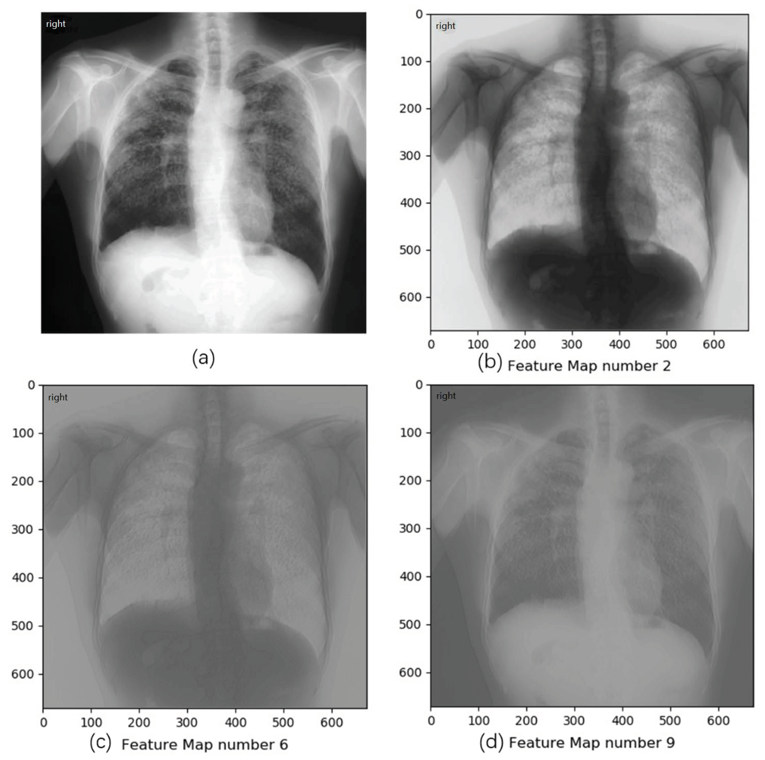
- We have explained diagnosis results by interpreting feature maps and visualizing suspected opacities on pneumoconiosis radiographs, which could provide a solid diagnostic reference for surgeons.
2. Materials and Methods
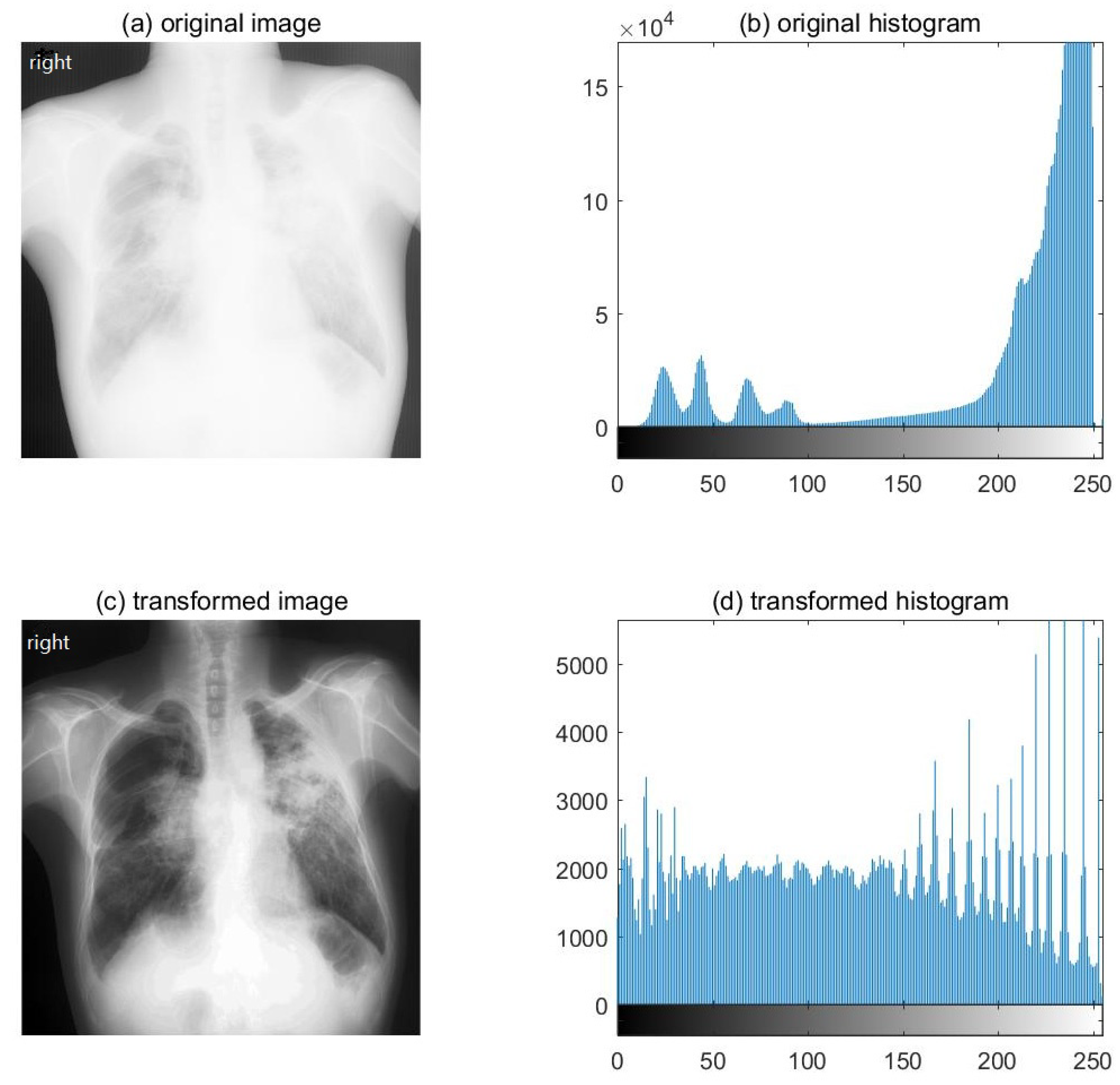
2.1. Dataset Preparing Process
2.2. Convolutional Models: ResNet and DenseNet
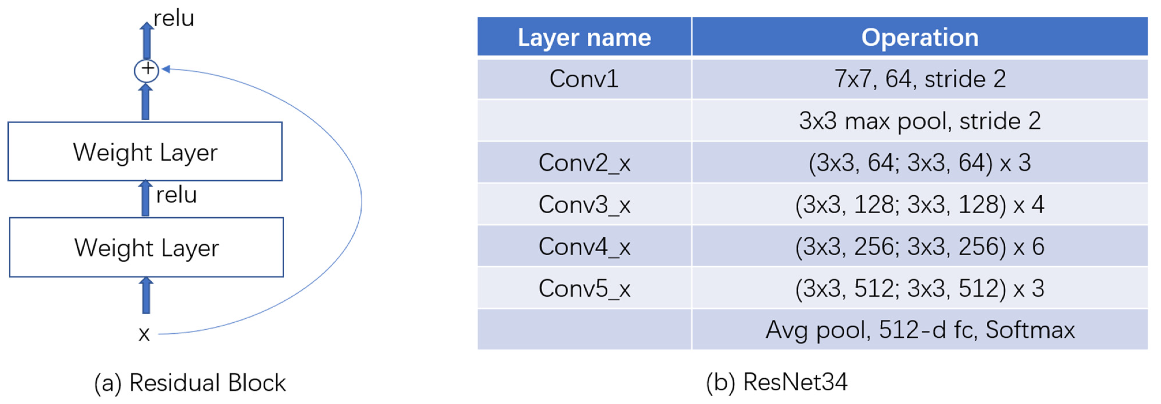
2.2.1. ResNet
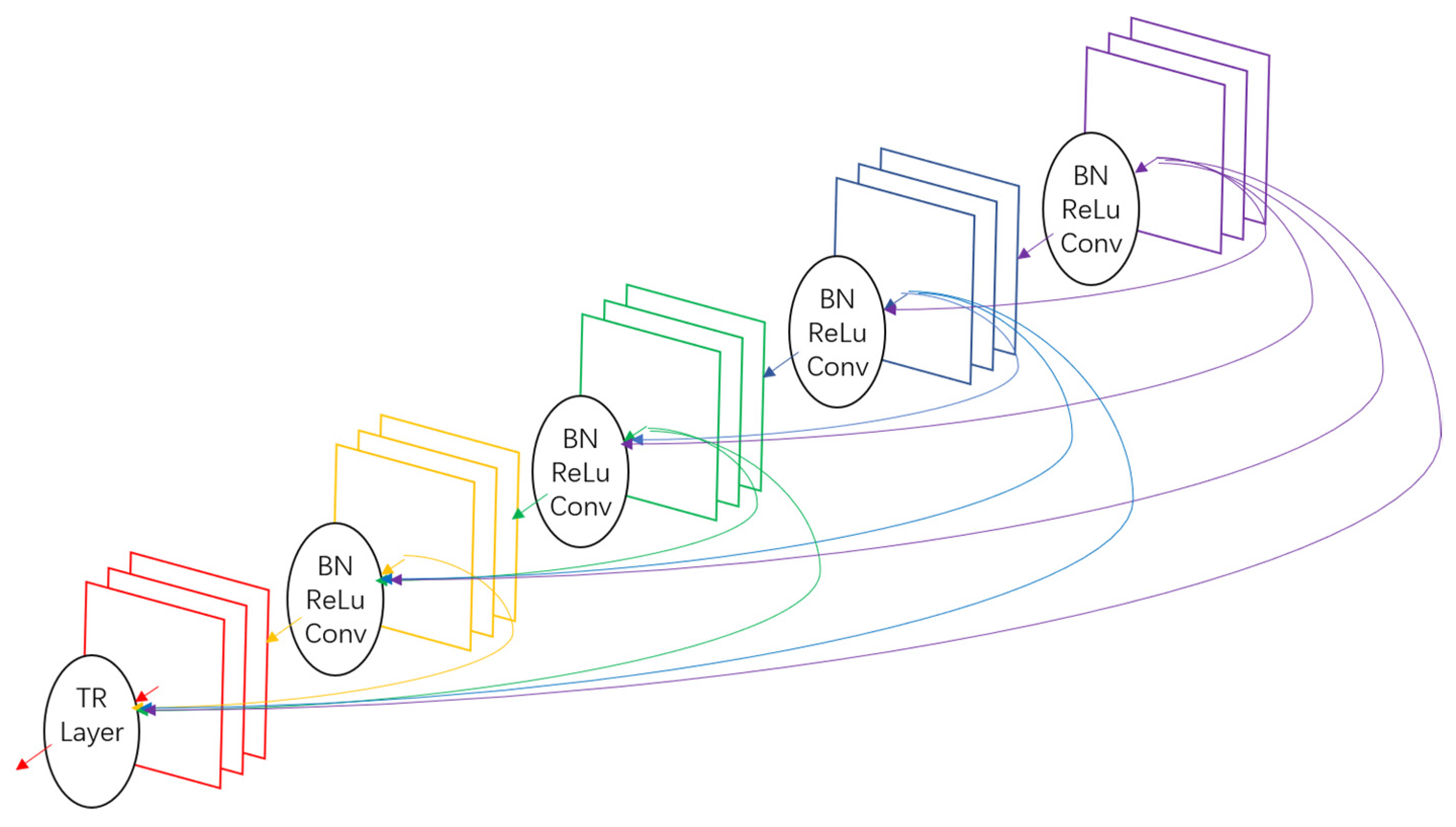
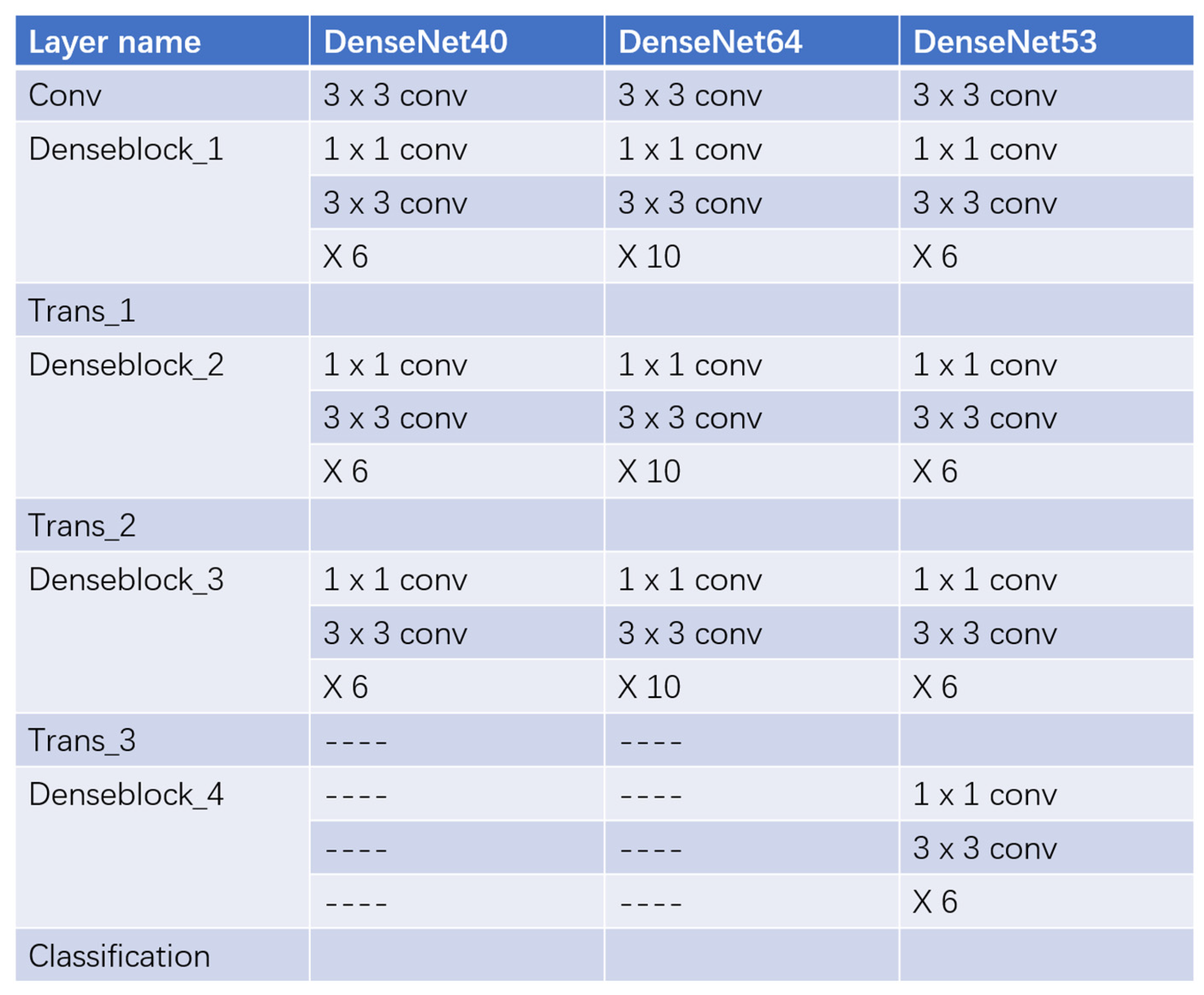
2.2.2. DenseNet
3. Results
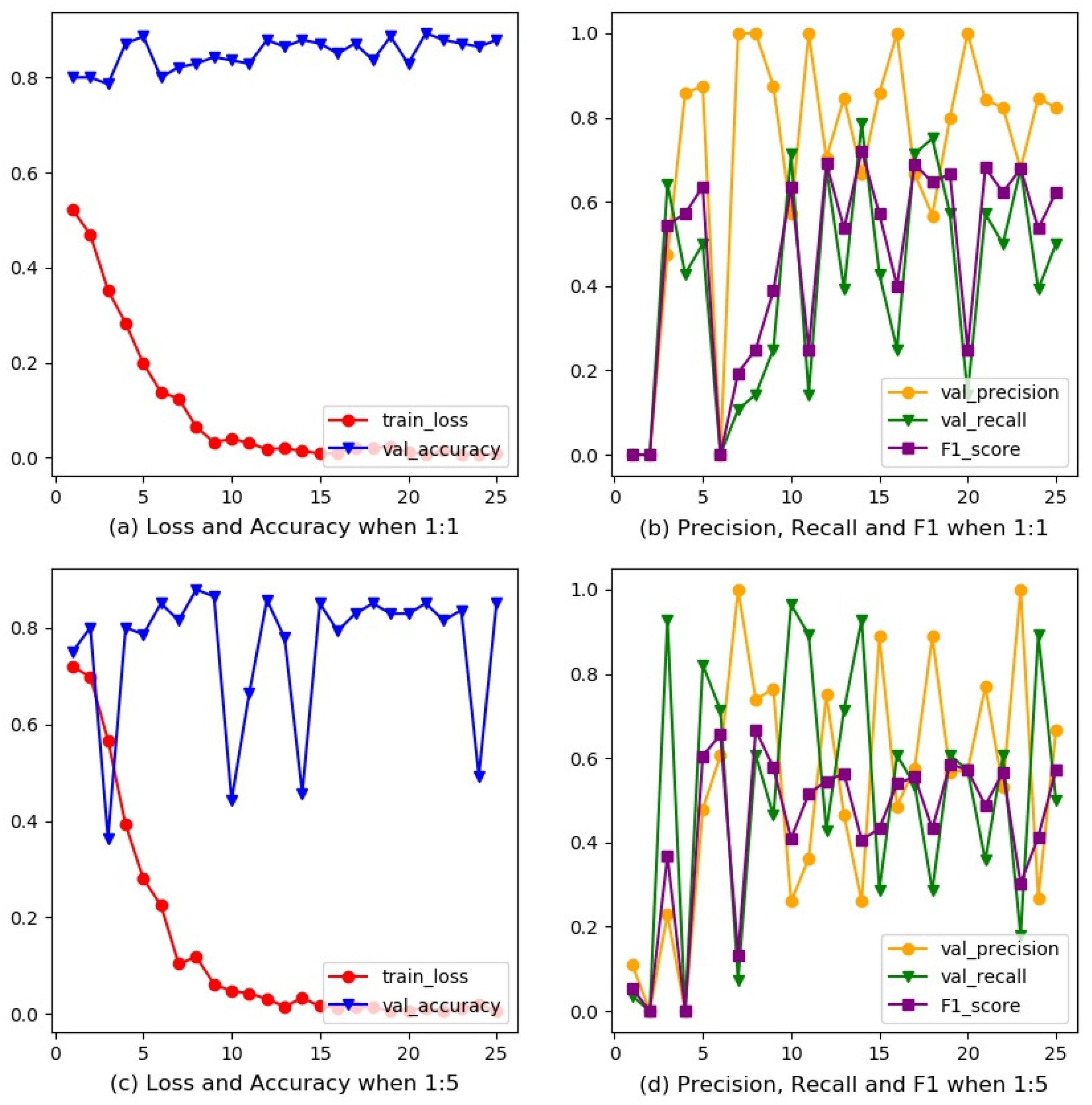
3.1. Rebalanced Training for ResNet
3.2. Refining Structure for DenseNet
3.2.1. Deeper Layers
3.2.2. Dropout Operation
3.2.3. Reduction Operation
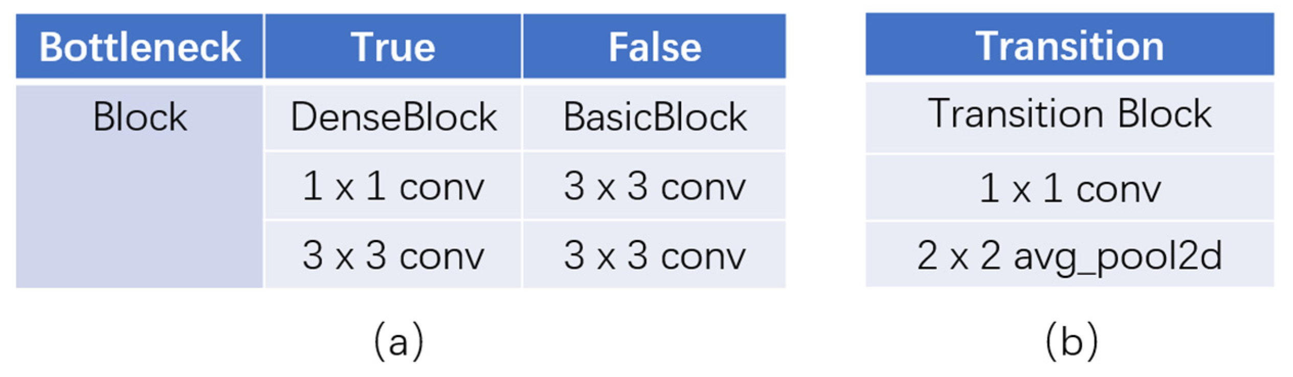
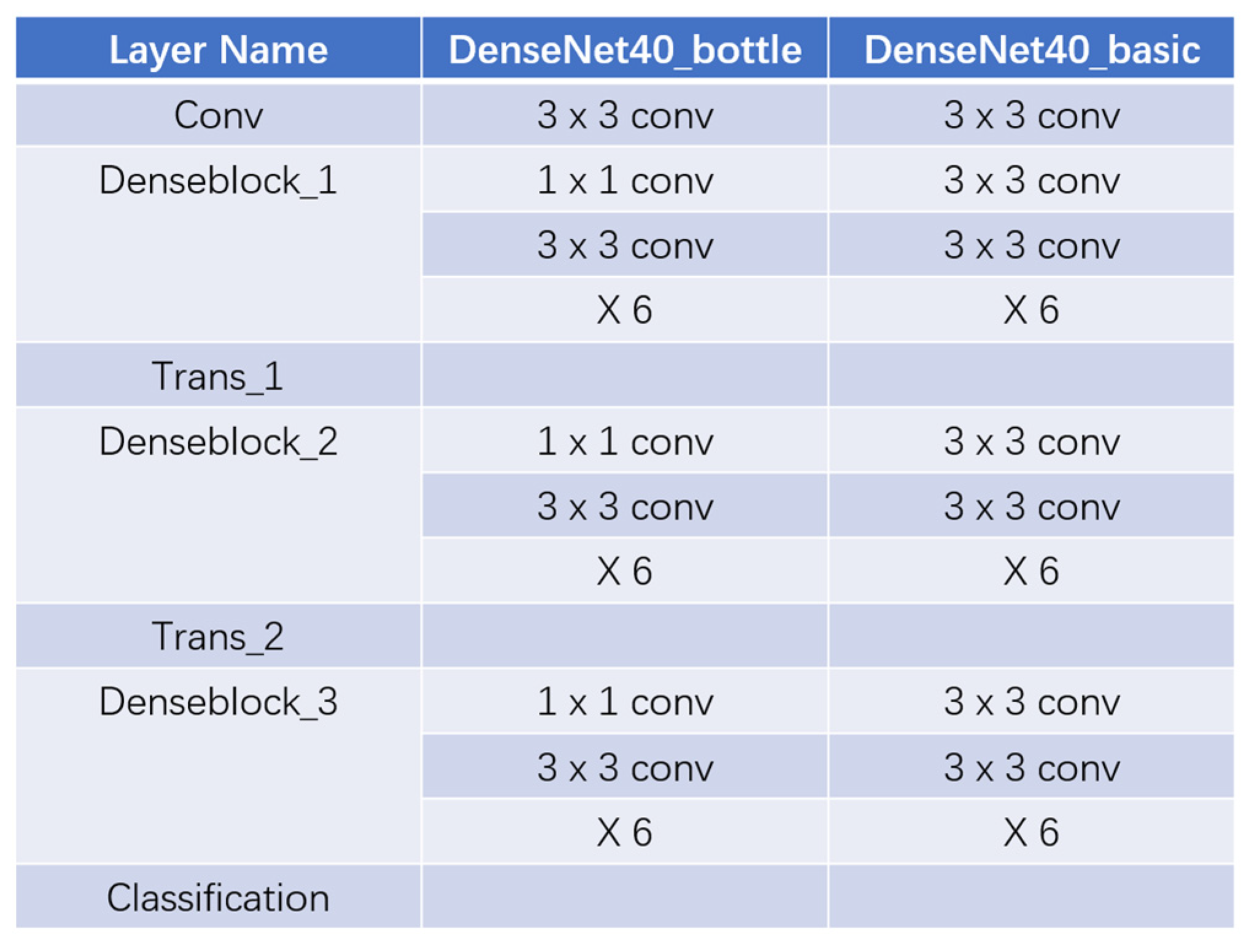
3.2.4. Bottleneck Blocks
4. Discussion
5. Conclusions
Author Contributions
Funding
Institutional Review Board Statement
Informed Consent Statement
Data Availability Statement
Conflicts of Interest
References
- Fletcher, C.M.; Elmes, P.C.; Fairbairn, A.S.; Wood, C.H. Significance of Respiratory Symptoms and the Diagnosis of Chronic Bronchitis in a Working Population. Br. Med. J. 1959, 2, 257–266. [Google Scholar] [CrossRef] [PubMed] [Green Version]
- YE, M.L.; WANG, Y.Y.; WAN, R.H. Research on Disease Burden of Pneumoconiosis Patients in Chongqing City. Mod. Prev. Med. 2011, 38, 840–842. [Google Scholar]
- Zhang, L.; Zhu, L.; Li, Z.H.; Li, J.Z.; Pan, H.W.; Zhang, S.F.; Qin, W.H.; He, L.H. Analysis on the Disease Burden and Its Impact Factors of Coal Worker’s Pneumoconiosis Inpatients. Beijing Da Xue Xue Bao J. Peking Univ. 2014, 46, 226–231. [Google Scholar]
- Maduskar, P.; Muyoyeta, M.; Ayles, H.; Hogeweg, L.; Peters-Bax, L.; Van Ginneken, B. Detection of tuberculosis using digital chest radiography: Automated reading vs. interpretation by clinical officers. Int. J. Tuberc. Lung Dis. 2013, 17, 1613–1620. [Google Scholar] [CrossRef] [PubMed]
- Yu, P.; Xu, H.; Zhu, Y.; Yang, C.; Sun, X.; Zhao, J. An Automatic Computer-Aided Detection Scheme for Pneumoconiosis on Digital Chest Radiographs. J. Digit. Imaging 2011, 24, 382–393. [Google Scholar] [CrossRef] [PubMed] [Green Version]
- Zhu, B.; Chen, H.; Chen, B.; Xu, Y.; Zhang, K. Support Vector Machine Model for Diagnosing Pneumoconiosis Based on Wavelet Texture Features of Digital Chest Radiographs. J. Digit. Imaging 2014, 27, 90–97. [Google Scholar] [CrossRef] [PubMed] [Green Version]
- Okumura, E.; Kawashita, I.; Ishida, T. Computerized Classification of Pneumoconiosis on Digital Chest Radiography Artificial Neural Network with Three Stages. J. Digit. Imaging 2017, 30, 413–426. [Google Scholar] [CrossRef] [PubMed]
- Lecun, Y.; Bottou, L.; Bengio, Y.; Haffner, P. Gradient-based learning applied to document recognition. Proc. IEEE 1998, 86, 2278–2324. [Google Scholar] [CrossRef] [Green Version]
- Krizhevsky, A.; Sutskever, I.; Hinton, G. ImageNet classification with deep convolutional neural networks. Commun. ACM 2017, 60, 84–90. [Google Scholar] [CrossRef]
- Zeiler, M.D.; Fergus, R. Visualizing and Understanding Convolutional Networks. In Proceedings of the IEEE Conference on European Conference on Computer Vision (ECCV), Zurich, Switzerland, 6–12 September 2014; pp. 818–833. [Google Scholar]
- Simonyan, K.; Zisserman, A. Very deep convolutional networks for large-scale image recognition. In Proceedings of the IEEE Conference on International Conference on Learning Representations (ICLR), San Diego, CA, USA, 7–9 May 2015. [Google Scholar]
- Christian, S.; Wei, L.; Yangqing, J.; Pierre, S.; Scott, R.; Dragomir, A.; Dumitru, E.; Vincent, V.; Andrew, R. Going Deeper with Convolutions. In Proceedings of the IEEE Conference on Computer Vision and Pattern Recognition (CVPR), Boston, MA, USA, 7–12 June 2015; pp. 1–9. [Google Scholar]
- He, K.; Zhang, X.; Ren, S.; Sun, J. Deep Residual Learning for Image Recognition. In Proceedings of the IEEE Conference on Computer Vision and Pattern Recognition (CVPR), Las Vegas, NV, USA, 26 June–1 July 2016; pp. 770–778. [Google Scholar]
- Huang, G.; Liu, Z.; Van Der Maaten, L.; Weinberger, K.Q. Densely Connected Convolutional Networks. In Proceedings of the 2017 IEEE Conference on Computer Vision and Pattern Recognition (CVPR), Honolulu, HI, USA, 21–26 July 2017; pp. 2261–2269. [Google Scholar]
- Tan, M.; Le, Q. EfficientNet: Rethinking Model Scaling for Convolutional Neural Networks. In Proceedings of the IEEE Conference on International Conference on Machine Learning (ICML), Long Beach, CA, USA, 9–15 June 2019. [Google Scholar]
- Cai, C.X.; Zhu, B.Y.; Chen, H. Computer-aided diagnosis for pneumoconiosis based on texture analysis on digital chest radiographs. In Proceedings of the International Conference on Measurement, Instrumentation and Automation (ICMIA), Guangzhou, China, 15–16 September 2012. [Google Scholar]
- Kermany, D.S.; Goldbaum, M.; Cai, W.; Valentim, C.C.; Liang, H.; Baxter, S.L.; McKeown, A.; Yang, G.; Wu, X.; Yan, F.; et al. Identifying Medical Diagnoses and Treatable Diseases by Image-Based Deep Learning. Cell 2018, 172, 1122–1131.e9. [Google Scholar] [CrossRef] [PubMed]
- Wang, X.; Yu, J.; Zhu, Q.; Li, S.; Zhao, Z.; Yang, B.; Pu, J. Potential of deep learning in assessing pneumoconiosis depicted on digital chest radiography. Occup. Environ. Med. 2020, 77, 597–602. [Google Scholar] [CrossRef] [PubMed]
- Müller, H.; Michoux, N.; Bandon, D.; Geissbuhler, A. A review of content-based image retrieval systems in medical Applications—Clinical benefits and future directions. Int. J. Med. Inform. 2004, 73, 1–23. [Google Scholar] [CrossRef] [PubMed]
- Gonzalez, R.C.; Richard, E. Woods. In Digital Image Processing, 4th ed.; Pearson: New York, NY, USA, 2018. [Google Scholar]
- Sermanet, P.; Eigen, D.; Zhang, X.; Mathieu, M.; Fergus, R.; LeCun, Y. OverFeat: Integrated Recognition, Localization and Detection Using Convolutional Networks. In Proceedings of the IEEE Conference on International Conference on Learning Representations (ICLR), Banff, AB, Canada, 14–16 April 2014. [Google Scholar]
- Shin, H.-C.; Roth, H.R.; Gao, M.; Lu, L.; Xu, Z.; Nogues, I.; Yao, J.; Mollura, D.; Summers, R.M. Deep Convolutional Neural Networks for Computer-Aided Detection: CNN Architectures, Dataset Characteristics and Transfer Learning. IEEE Trans. Med. Imaging 2016, 35, 1285–1298. [Google Scholar] [CrossRef] [Green Version]
- Guo, Y.; Liu, Y.; Oerlemans, A.; Lao, S.; Wu, S.; Lew, M.S. Deep learning for visual understanding: A review. Neurocomputing 2016, 187, 27–48. [Google Scholar] [CrossRef]
- Wilson, H.R.; Cowan, J.D. Excitatory and Inhibitory Interactions in Localized Populations of Model Neurons. Biophys. J. 1972, 12, 1–24. [Google Scholar] [CrossRef] [Green Version]
- McCulloch, W.S.; Pitts, W. A logical calculus of the ideas immanent in nervous activity. Bull. Math. Biol. 1990, 52, 99–115. [Google Scholar] [CrossRef]
- Glorot, X.; Bordes, A.; Bengio, Y. Deep sparse rectifier networks. In Proceedings of the 14th International Conference on Artificial Intelligence and Statistics, Ft. Lauderdale, FL, USA, 11–13 April 2011; Volume 15, pp. 315–323. [Google Scholar]
- Goodfellow, I.; Bengio, Y.; Courville, A. Deep Learning (Adaptive Computation and Machine Learning); MIT P: Cambridge, MA, USA, 2016. [Google Scholar]
- Kaiming, H.; Jian, S. Convolutional neural networks at constrained time cost. In Proceedings of the IEEE Conference on Computer Vision and Pattern Recognition (CVPR), Boston, MA, USA, 7–12 June 2015; pp. 5353–5360. [Google Scholar]
- Rubinstein, R. The Cross-Entropy Method for Combinatorial and Continuous Optimization. Methodol. Comput. Appl. Probab. 1999, 1, 127–190. [Google Scholar] [CrossRef]
- Ioffe, S.; Szegedy, C. Batch normalization: Accelerating deep network training by reducing internal covariate shift. In Proceedings of the IEEE Conference on International Conference on Machine Learning (ICML), Lille, France, 6–11 July 2015. [Google Scholar]
- Litjens, G.; Kooi, T.; Bejnordi, B.E.; Setio, A.A.A.; Ciompi, F.; Ghafoorian, M.; van der Laak, J.A.W.M.; van Ginneken, B.; Sánchez, C.I.S. A survey on deep learning in medical image analysis. Med. Image Anal. 2017, 42, 60–88. [Google Scholar] [CrossRef] [PubMed] [Green Version]
- De Vuyst, P.; Dumortier, P.; Swaen, G.M.; Pairon, J.C.; Brochard, P. Respiratory health effects of man-made vitreous (mineral) fibres. Eur. Respir. J. 1995, 8, 2149–2173. [Google Scholar] [CrossRef] [PubMed] [Green Version]


| Metrics | Definition |
|---|---|
| TP | True Positive. Samples predicted to be positive with a positive ground truth label. |
| FP | False Positive. Samples predicted to be positive with a negative ground truth label. |
| FN | False Negative. Samples predicted to be negative with a positive ground truth label. |
| TN | True Negative. Samples predicted to be negative with a negative ground truth label. |
| Accuracy | |
| Precision | |
| Recall | |
| F1 Score |
| ResNet34 | ResNet34 | |
|---|---|---|
| n | 1 | 5 |
| Accuracy | 0.893 | 0.879 |
| Precision | 0.842 | 0.739 |
| Recall | 0.571 | 0.607 |
| F1 Score | 0.681 | 0.667 |
| Model | DenseNet40 | DenseNet64 | DenseNet53 |
|---|---|---|---|
| Accuracy | 0.843 | 0.871 | 0.886 |
| Precision | 0.714 | 0.750 | 0.833 |
| Recall | 0.357 | 0.536 | 0.536 |
| F1 Score | 0.476 | 0.625 | 0.652 |
| Drop rate | 0 | 0.25 |
| Accuracy | 0.886 | 0.843 |
| Precision | 0.833 | 0.714 |
| Recall | 0.536 | 0.357 |
| F1 Score | 0.652 | 0.476 |
| Reduction | 0.25 | 0.5 | 1 |
| Accuracy | 0.886 | 0.871 | 0.836 |
| Precision | 0.833 | 0.692 | 0.647 |
| Recall | 0.536 | 0.643 | 0.393 |
| F1 Score | 0.652 | 0.667 | 0.489 |
| Bottleneck | False | True |
|---|---|---|
| Accuracy | 0.836 | 0.886 |
| Precision | 0.600 | 0.833 |
| Recall | 0.536 | 0.536 |
| F1 Score | 0.566 | 0.652 |
Publisher’s Note: MDPI stays neutral with regard to jurisdictional claims in published maps and institutional affiliations. |
© 2021 by the authors. Licensee MDPI, Basel, Switzerland. This article is an open access article distributed under the terms and conditions of the Creative Commons Attribution (CC BY) license (https://creativecommons.org/licenses/by/4.0/).
Share and Cite
Hao, C.; Jin, N.; Qiu, C.; Ba, K.; Wang, X.; Zhang, H.; Zhao, Q.; Huang, B. Balanced Convolutional Neural Networks for Pneumoconiosis Detection. Int. J. Environ. Res. Public Health 2021, 18, 9091. https://doi.org/10.3390/ijerph18179091
Hao C, Jin N, Qiu C, Ba K, Wang X, Zhang H, Zhao Q, Huang B. Balanced Convolutional Neural Networks for Pneumoconiosis Detection. International Journal of Environmental Research and Public Health. 2021; 18(17):9091. https://doi.org/10.3390/ijerph18179091
Chicago/Turabian StyleHao, Chaofan, Nan Jin, Cuijuan Qiu, Kun Ba, Xiaoxi Wang, Huadong Zhang, Qi Zhao, and Biqing Huang. 2021. "Balanced Convolutional Neural Networks for Pneumoconiosis Detection" International Journal of Environmental Research and Public Health 18, no. 17: 9091. https://doi.org/10.3390/ijerph18179091
APA StyleHao, C., Jin, N., Qiu, C., Ba, K., Wang, X., Zhang, H., Zhao, Q., & Huang, B. (2021). Balanced Convolutional Neural Networks for Pneumoconiosis Detection. International Journal of Environmental Research and Public Health, 18(17), 9091. https://doi.org/10.3390/ijerph18179091