
Near-Source Risk Functions for Particulate Matter Are Critical When Assessing the Health Benefits of Local Abatement Strategies


Abstract
:1. Introduction
2. Materials and Methods
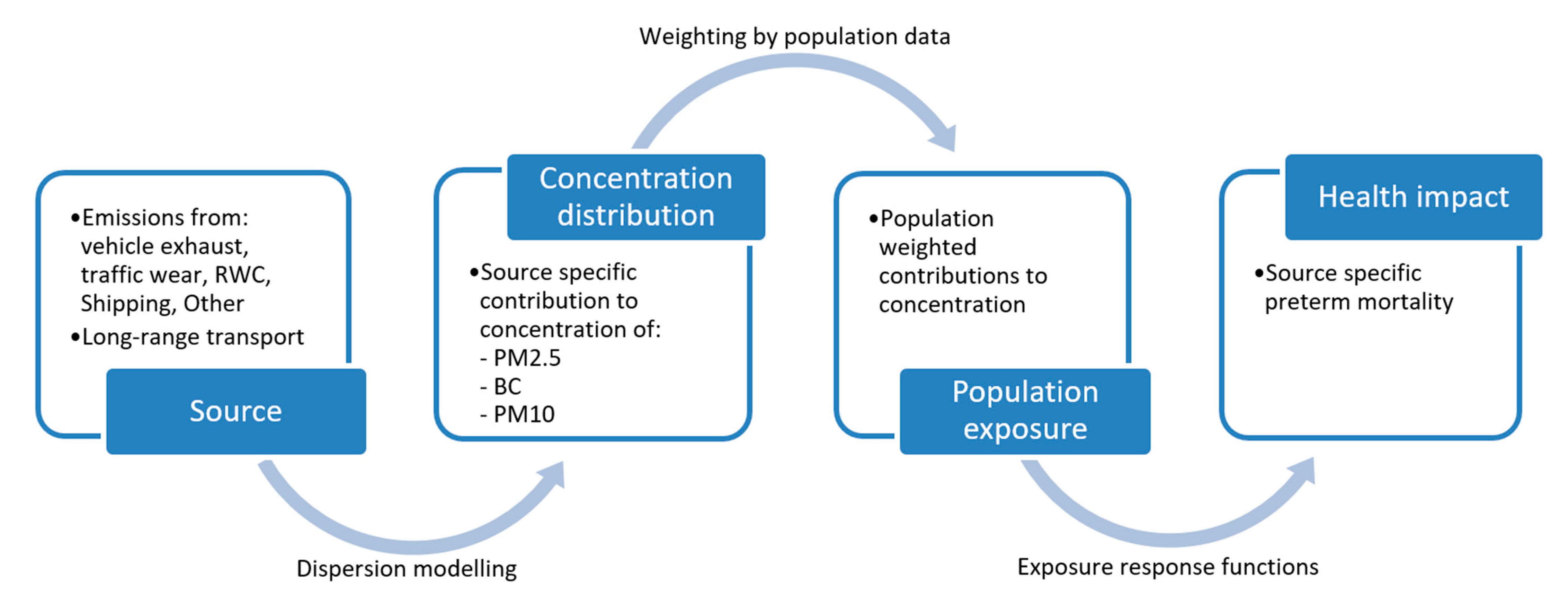
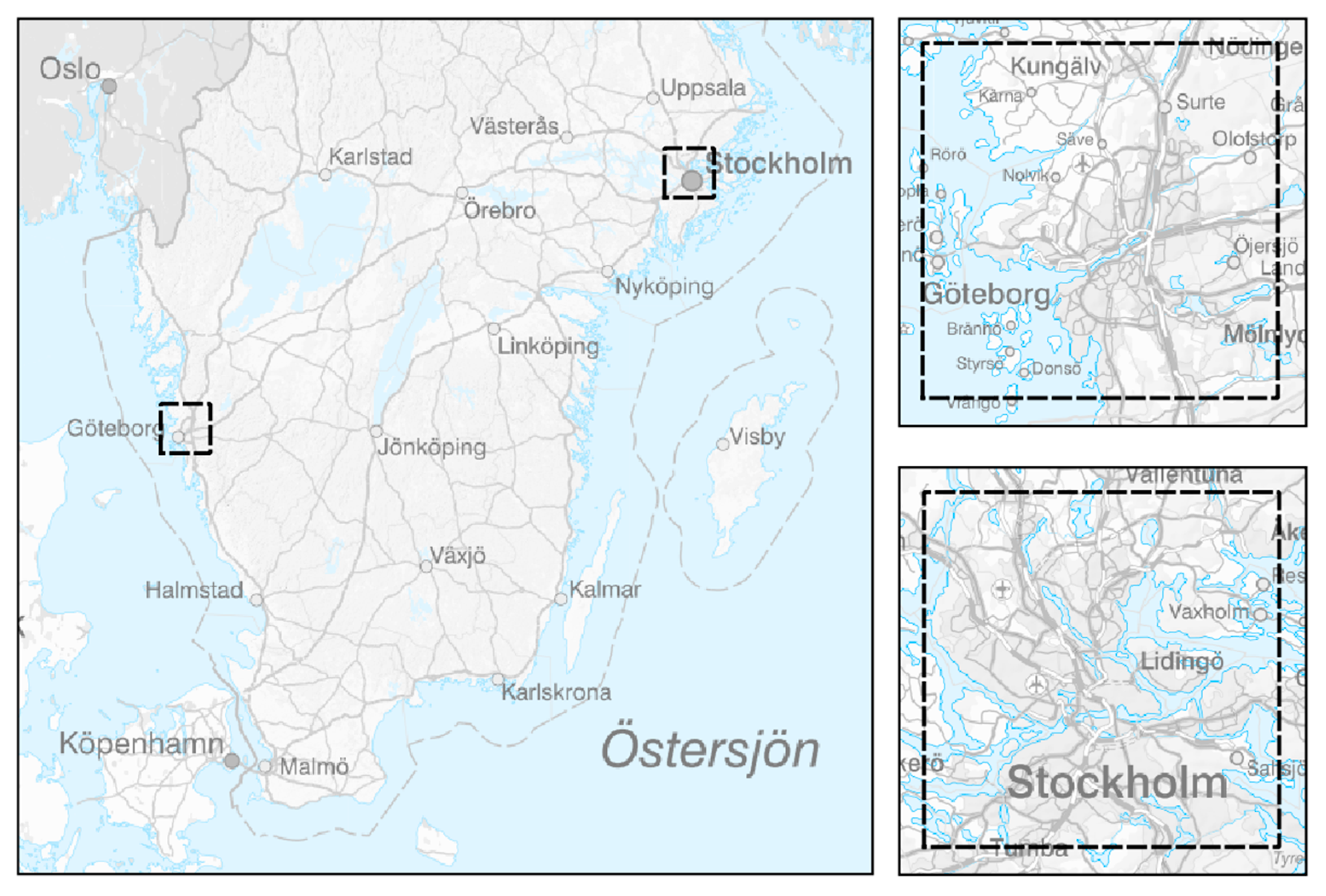
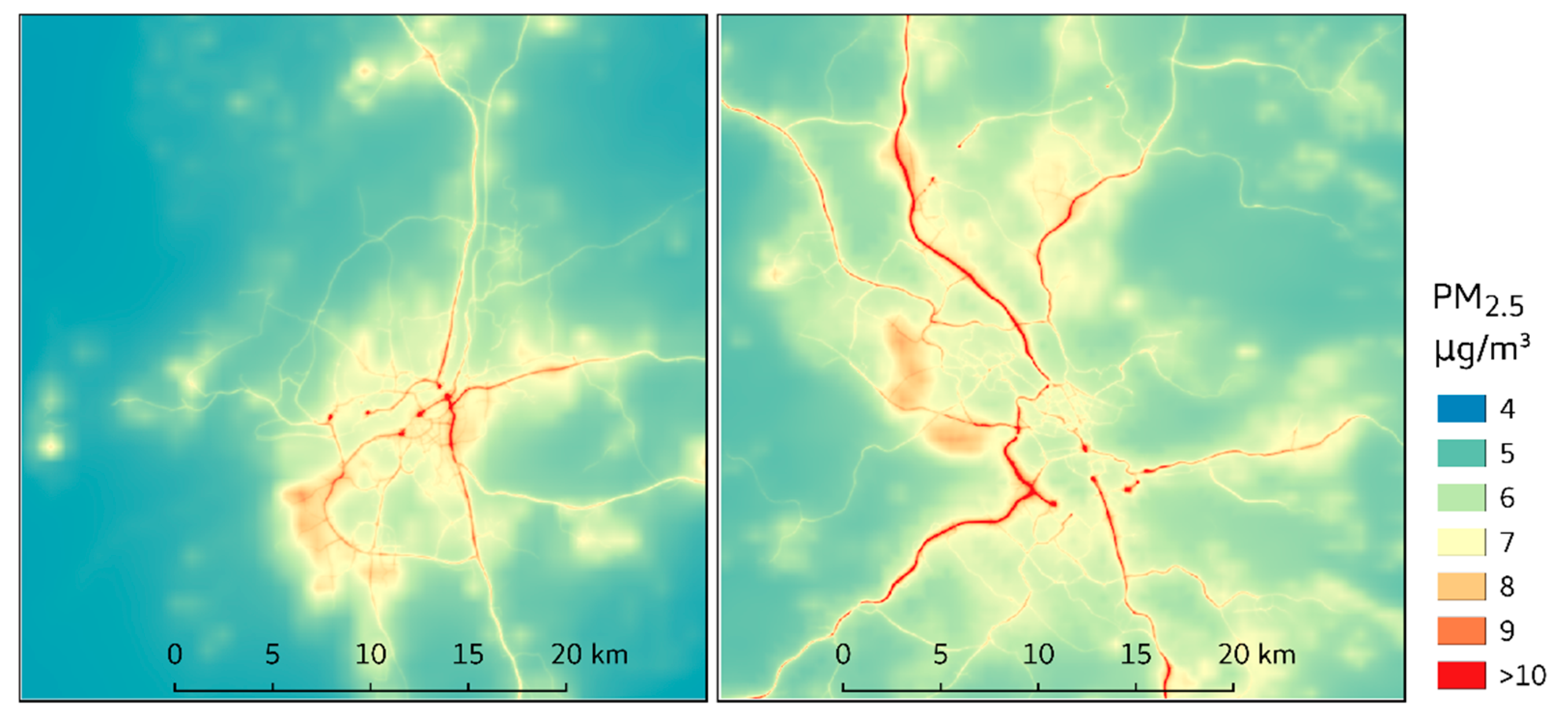
2.1. Population Exposure
- Residential wood combustion (RWC);
- Road traffic (exhaust);
- Road traffic (wear);
- Shipping;
- Other local sources.
2.2. Abatement Strategies
2.2.1. Introduction of Congestion Charges
2.2.2. Reduced Use of Studded Tires
2.2.3. Electrification of Light Vehicles
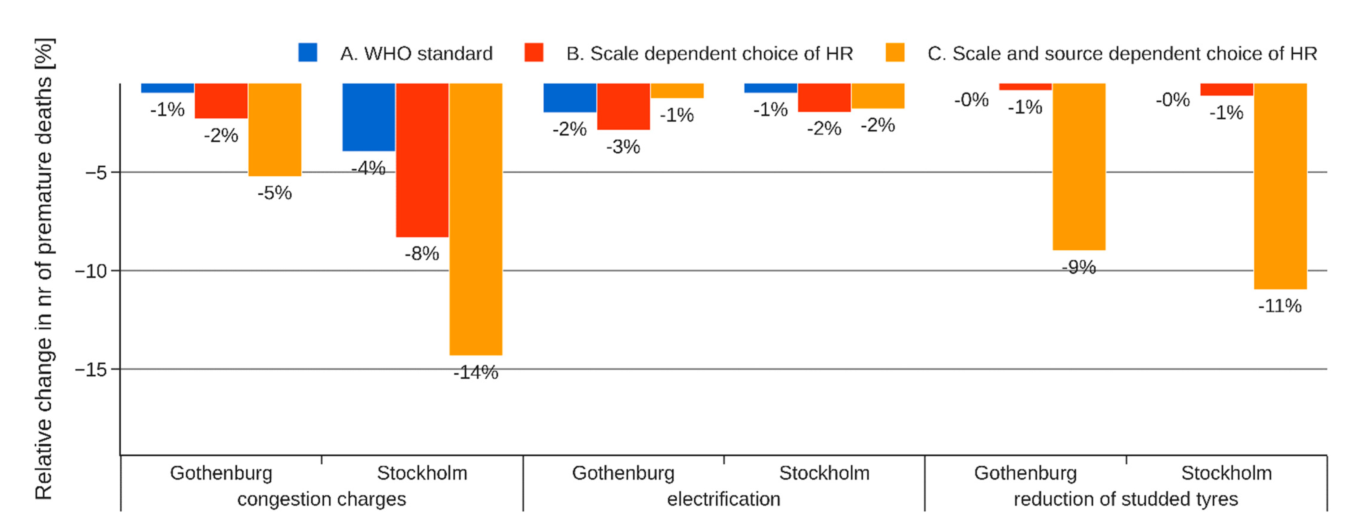
2.3. Health Impact Analysis
- WHO standardThe same 1.08 (CI 95% 1.06–1.09) HR [32] is applied for PM2.5 regardless of source and origin of the particles;
- Separation by distance to sourceHRs based on near-source and regional decompositions [28] are applied to local contributions and LRT, respectively;
- Separation by source category and distance
3. Results
3.1. Evaluation of Abatement Strategies
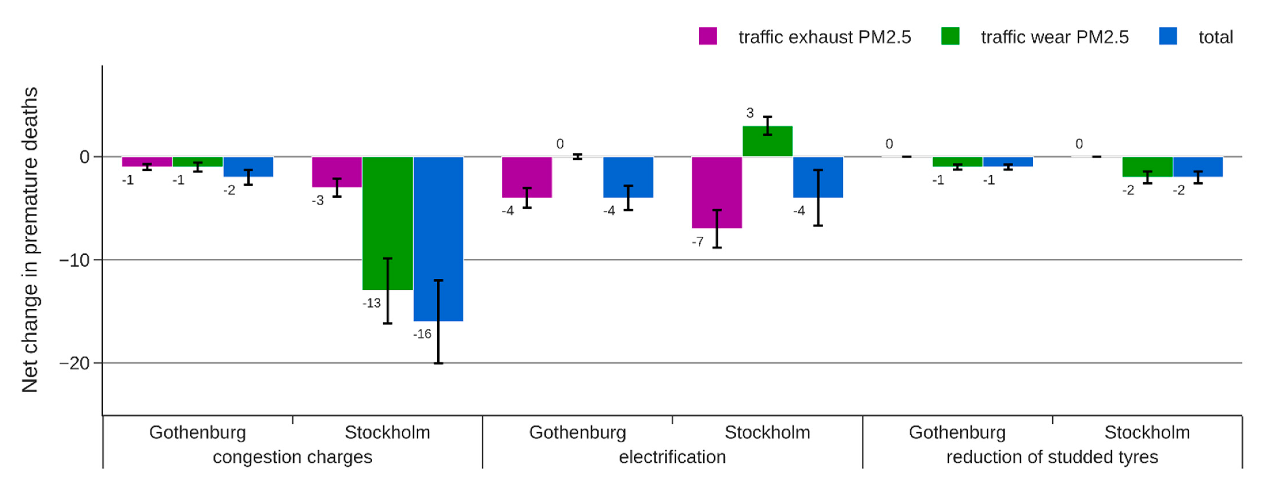
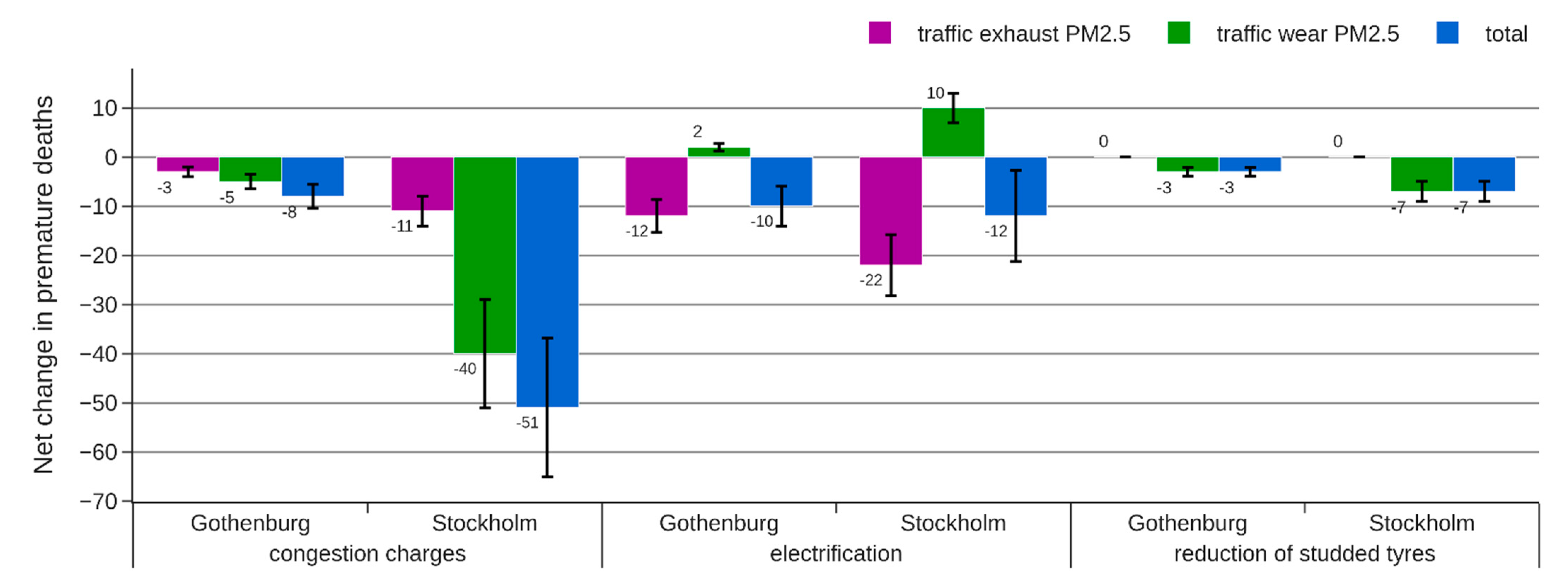
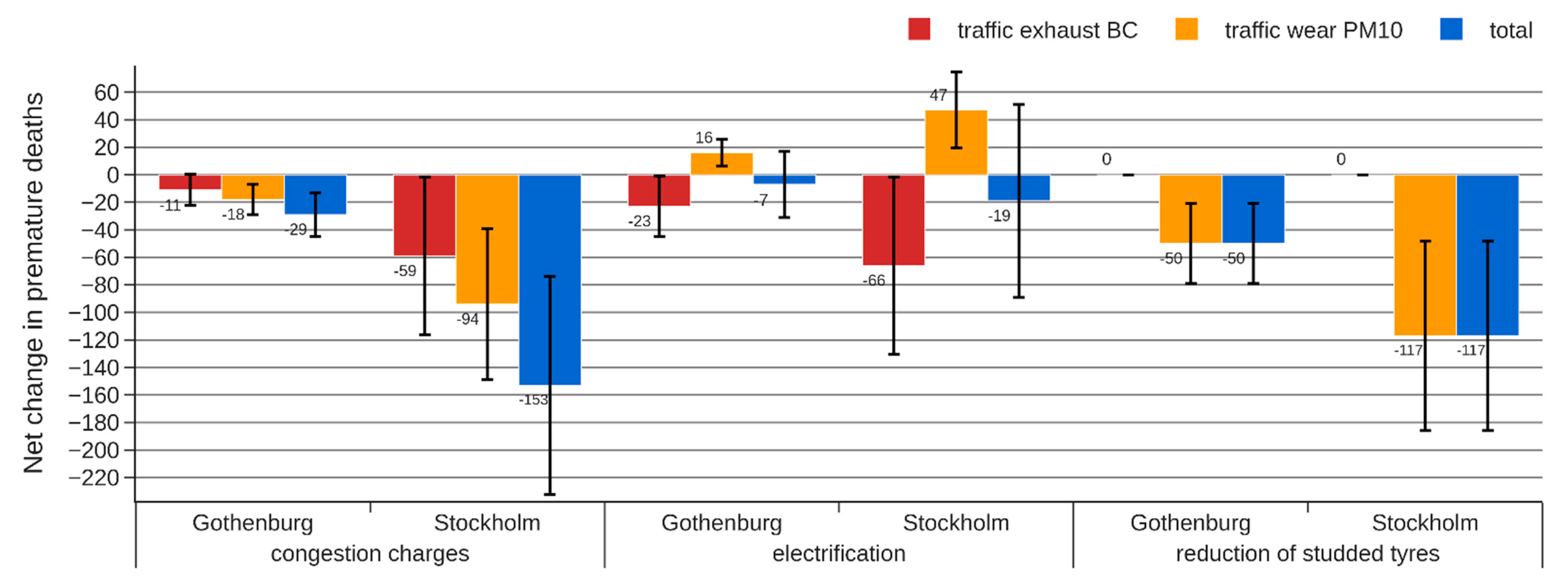
3.2. Source-Specific Change in Mortality
4. Discussion
5. Conclusions
Supplementary Materials
Author Contributions
Funding
Institutional Review Board Statement
Informed Consent Statement
Data Availability Statement
Conflicts of Interest
Appendix A

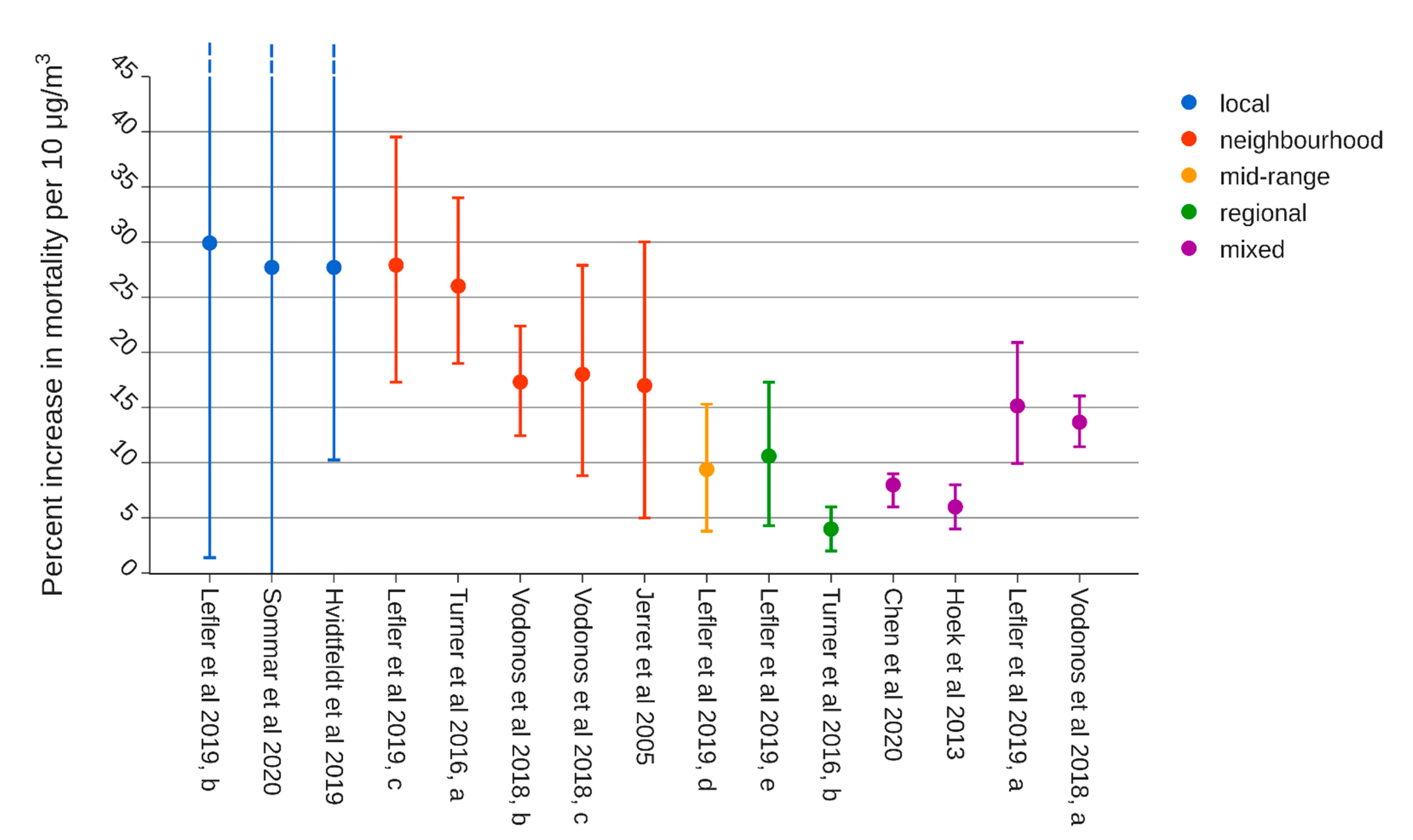
| Reference | Spatial Scale | HR |
|---|---|---|
| Chen et al. [32] | mixed | 1.08 (1.06–1.09) |
| Hoek et al. [5] | mixed | 1.06 (1.04–1.08) |
| Lefler et al. [29], a | mixed | 1.15 (1.10–1.21) |
| Lefler et al. [29], b | local | 1.30 (1.10–1.66) |
| Lefler et al. [29], c | neighborhood | 1.28 (1.17–1.40) |
| Lefler et al. [29], d | mid-range | 1.09 (1.04–1.15) |
| Lefler et al. [29], e | regional | 1.11 (1.04–1.17) |
| Turner et al. [28], a | local | 1.26 (1.19–1.34) |
| Turner et al. [28], b | regional | 1.04 (1.02–1.06) |
| Vodonos et al. [30], a | mixed | 1.14 (1.11–1.16) 1 |
| Vodonos et al. [30], b | neighborhood | 1.17 (1.12–1.22) 1,2 |
| Vodonos et al. [30], c | neighborhood | 1.18 (1.19–1.28) 1,3 |
| Sommar et al. [33] | local | 1.28 (−0.83–1.96) |
| Hvidtfeldt et al. [42] | local | 1.28 (1.10–1.46) |
| Jerret et al. [25] | neighborhood | 1.17 (1.05–1.30) |
References
- GBD 2019 Risk Factors Collaborators. Global burden of 87 risk factors in 204 countries and territories, 1990–2019: A systematic analysis for the Global Burden of Disease Study 2019. Lancet 2020, 396, 1223–1249. [Google Scholar] [CrossRef]
- Vohra, K.; Vodonos, A.; Schwartz, J.; Marais, E.A.; Sulprizio, M.P.; Mickley, L.J. Global mortality from outdoor fine particle pollution generated by fossil fuel combustion: Results from GEOS-Chem. Environ. Res. 2021, 195, 110754. [Google Scholar] [CrossRef] [PubMed]
- World Health Organization (Ed.) Air Quality Guidelines: Global Update 2005: Particulate Matter, Ozone, Nitrogen Dioxide, and Sulfur Dioxide; World Health Organization: Copenhagen, Denmark, 2006; ISBN 978-92-890-2192-0. [Google Scholar]
- Health Risks of Air Pollution in Europe–HRAPIE Project. Recommendations for Concentration–Response Functions for Cost–Benefit Analysis of Particulate Matter, Ozone and Nitrogen Dioxide; WHO Regional Office for Europe: Copenhagen, Denmark, 2013. [Google Scholar]
- Hoek, G.; Krishnan, R.M.; Beelen, R.; Peters, A.; Ostro, B.; Brunekreef, B.; Kaufman, J.D. Long-term air pollution exposure and cardio- respiratory mortality: A review. Environ. Health 2013, 12, 43. [Google Scholar] [CrossRef] [PubMed] [Green Version]
- Janssen, N.A.; Hoek, G.; Simic-Lawson, M.; Fischer, P.; Van Bree, L.; ten Brink, H.; Keuken, M.; Atkinson, R.W.; Anderson, H.R.; Brunekreef, B.; et al. Black Carbon as an Additional Indicator of the Adverse Health Effects of Airborne Particles Compared with PM10and PM2.5. Environ. Health Perspect. 2011, 119, 1691–1699. [Google Scholar] [CrossRef] [PubMed] [Green Version]
- Chen, J.; Rodopoulou, S.; de Hoogh, K.; Strak, M.; Andersen, Z.J.; Atkinson, R.; Bauwelinck, M.; Bellander, T.; Brandt, J.; Cesaroni, G.; et al. Long-Term Exposure to Fine Particle Elemental Components and Natural and Cause-Specific Mortality—A Pooled Analysis of Eight European Cohorts within the ELAPSE Project. Environ. Health Perspect. 2021, 129, 47009. [Google Scholar] [CrossRef]
- Forsberg, B.; Hansson, H.-C.; Johansson, C.; Areskoug, H.; Persson, K.; Järvholm, B. Comparative Health Impact Assessment of Local and Regional Particulate Air Pollutants in Scandinavia. Ambio 2005, 34, 11–19. [Google Scholar] [CrossRef]
- Fann, N.; Coffman, E.; Timin, B.; Kelly, J.T. The estimated change in the level and distribution of PM2.5-attributable health impacts in the United States: 2005–2014. Environ. Res. 2018, 167, 506–514. [Google Scholar] [CrossRef]
- Johansson, C.; Burman, L.; Forsberg, B. The effects of congestions tax on air quality and health. Atmos. Environ. 2009, 43, 4843–4854. [Google Scholar] [CrossRef]
- Orru, H.; Lövenheim, B.; Johansson, C.; Forsberg, B. Potential health impacts of changes in air pollution exposure associated with moving traffic into a road tunnel. J. Expo. Sci. Environ. Epidemiol. 2015, 25, 524–531. [Google Scholar] [CrossRef] [Green Version]
- Brønnum-Hansen, H.; Bender, A.M.; Andersen, Z.J.; Sørensen, J.; Bonlokke, J.H.; Boshuizen, H.; Becker, T.; Diderichsen, F.; Loft, S. Assessment of impact of traffic-related air pollution on morbidity and mortality in Copenhagen Municipality and the health gain of reduced exposure. Environ. Int. 2018, 121, 973–980. [Google Scholar] [CrossRef]
- Haluza, D.; Kaiser, A.; Moshammer, H.; Flandorfer, C.; Kundi, M.; Neuberger, M. Estimated health impact of a shift from light fuel to residential wood-burning in Upper Austria. J. Expo. Sci. Environ. Epidemiol. 2012, 22, 339–343. [Google Scholar] [CrossRef]
- Segersson, D.; Eneroth, K.; Gidhagen, L.; Johansson, C.; Omstedt, G.; Nylén, A.E.; Forsberg, B. Health Impact of PM10, PM2.5 and Black Carbon Exposure Due to Different Source Sectors in Stockholm, Gothenburg and Umea, Sweden. Int. J. Environ. Res. Public Health 2017, 14, 742. [Google Scholar] [CrossRef] [PubMed] [Green Version]
- Börjesson, M.; Eliasson, J.; Hugosson, M.B.; Brundell-Freij, K. The Stockholm congestion charges—5 years on. Effects, acceptability and lessons learnt. Transp. Policy 2012, 20, 1–12. [Google Scholar] [CrossRef]
- West, J.; Börjesson, M. The Gothenburg congestion charges: Cost–benefit analysis and distribution effects. Transportation 2018, 47, 145–174. [Google Scholar] [CrossRef] [Green Version]
- Denby, B.; Sundvor, I.; Johansson, C.; Pirjola, L.; Ketzel, M.; Norman, M.; Kupiainen, K.; Gustafsson, M.; Blomqvist, G.; Omstedt, G. A coupled road dust and surface moisture model to predict non-exhaust road traffic induced particle emissions (NORTRIP). Part 1: Road dust loading and suspension modelling. Atmos. Environ. 2013, 77, 283–300. [Google Scholar] [CrossRef]
- Norman, M.; Sundvor, I.; Denby, B.; Johansson, C.; Gustafsson, M.; Blomqvist, G.; Janhäll, S. Modelling road dust emission abatement measures using the NORTRIP model: Vehicle speed and studded tyre reduction. Atmos. Environ. 2016, 134, 96–108. [Google Scholar] [CrossRef]
- Stockholm City Strategy for a Fossil-Fuel Free Stockholm by 2040; City Executive Office: Stockholm, Sweden, 2017.
- Requia, W.J.; Arain, A.; Koutrakis, P.; Dalumpines, R. Assessing particulate matter emissions from future electric mobility and potential risk for human health in Canadian metropolitan area. Air Qual. Atmos. Health 2018, 11, 1009–1019. [Google Scholar] [CrossRef]
- Maesano, C.; Morel, G.; Matynia, A.; Ratsombath, N.; Bonnety, J.; Legros, G.; Da Costa, P.; Prud’Homme, J.; Annesi-Maesano, I. Impacts on human mortality due to reductions in PM10 concentrations through different traffic scenarios in Paris, France. Sci. Total Environ. 2020, 698, 134257. [Google Scholar] [CrossRef]
- Simons, A. Road transport: New life cycle inventories for fossil-fuelled passenger cars and non-exhaust emissions in ecoinvent v3. Int. J. Life Cycle Assess. 2013, 21, 1299–1313. [Google Scholar] [CrossRef]
- Kriit, H.; Forsberg, B.; Åström, S.; Sommar, J.; Svensson, M.; Johansson, C. A Health Economic Assessment of Air Pollution Effects under Climate Neutral Vehicle Fleet Scenarios in Stockholm, Sweden. J. Transp. Health 2021, 22, 101084. [Google Scholar] [CrossRef]
- Bickel, P.; Friedrich, R.; Extern, E. Methodology 2005 Update; European Commission: Brussels, Belgium, 2005. [Google Scholar]
- Pope, C.A.; Thun, M.J.; Namboodiri, M.M.; Dockery, D.W.; Evans, J.S.; Speizer, F.E.; Heath, C.W. Particulate Air Pollution as a Predictor of Mortality in a Prospective Study of U.S. Adults. Am. J. Respir. Crit. Care Med. 1995, 151, 669–674. [Google Scholar] [CrossRef]
- Pope, C.A., 3rd; Burnett, R.T.; Thun, M.J.; Calle, E.E.; Krewski, D.; Ito, K.; Thurston, G.D. Lung cancer, cardiopulmonary mortality, and long-term exposure to fine particulate air pollution. J. Am. Med. Assoc. 2002, 287, 1132–1141. [Google Scholar] [CrossRef] [PubMed] [Green Version]
- Jerrett, M.; Burnett, R.T.; Ma, R.; Pope, C.A.; Krewski, D.; Newbold, K.B.; Thurston, G.; Shi, Y.; Finkelstein, N.; Calle, E.E.; et al. Spatial Analysis of Air Pollution and Mortality in Los Angeles. Epidemiology 2005, 16, 727–736. [Google Scholar] [CrossRef] [PubMed]
- Turner, M.C.; Jerrett, M.; Pope, C.A.; Krewski, D.; Gapstur, S.M.; Diver, W.R.; Beckerman, B.S.; Marshall, J.D.; Su, J.; Crouse, D.; et al. Long-Term Ozone Exposure and Mortality in a Large Prospective Study. Am. J. Respir. Crit. Care Med. 2016, 193, 1134–1142. [Google Scholar] [CrossRef] [Green Version]
- Lefler, J.S.; Higbee, J.D.; Burnett, R.T.; Ezzati, M.; Coleman, N.C.; Mann, D.D.; Marshall, J.D.; Bechle, M.; Wang, Y.; Robinson, A.L.; et al. Air pollution and mortality in a large, representative U.S. cohort: Multiple-pollutant analyses, and spatial and temporal decompositions. Environ. Health 2019, 18, 1–11. [Google Scholar] [CrossRef] [PubMed] [Green Version]
- Vodonos, A.; Abu Awad, Y.; Schwartz, J. The concentration-response between long-term PM2.5 exposure and mortality; A meta-regression approach. Environ. Res. 2018, 166, 677–689. [Google Scholar] [CrossRef]
- Burnett, R.; Chen, H.; Szyszkowicz, M.; Fann, N.; Hubbell, B.; Pope, C.A.; Apte, J.; Brauer, M.; Cohen, A.; Weichenthal, S.; et al. Global estimates of mortality associated with long-term exposure to outdoor fine particulate matter. Proc. Natl. Acad. Sci. USA 2018, 115, 9592–9597. [Google Scholar] [CrossRef] [Green Version]
- Chen, J.; Hoek, G. Long-term exposure to PM and all-cause and cause-specific mortality: A systematic review and meta-analysis. Environ. Int. 2020, 143, 105974. [Google Scholar] [CrossRef]
- Sommar, J.N.; Andersson, E.M.; Andersson, N.; Sällsten, G.; Stockfeldt, L.; Ljungman, P.L.S.; Segersson, D.; Eneroth, K.; Gidhagen, L.; Molnár, P.; et al. Long-Term Exposure to Particulate Air Pollution and Black Carbon in Relation to Natural and Cause Specific Mortality: A Multi-Cohort Study in Sweden. Resubmitted Rev. 2021. [Google Scholar]
- Saarikoski, S.; Niemi, J.V.; Aurela, M.; Pirjola, L.; Kousa, A.; Rönkkö, T.; Timonen, H. Sources of Black Carbon at Residential and Traffic Environments. Atmos. Chem. Phys. Discuss 2021. under review. [Google Scholar] [CrossRef]
- Air Quality Expert Group Non-Exhaust Emissions from Road Traffic; Department for Environment, Food and Rural Affairs; Scottish Government; Welsh Government; and Department of the Environment in Northern Ireland: London, UK, 2019.
- Hoek, G.; Beleen, R.; de Hoogh, K.; Vienneau, D.; Gulliver, J.; Fischer, P.; Briggs, D. A review of land-use regression models to assess spatial variationof outdoor air pollution. Atmos. Environ. 2008, 42, 7561–7578. [Google Scholar] [CrossRef]
- US EPA Integrated Science Assessment (ISA) for Particulate Matter (Final Report, Dec 2019); U.S. Environmental Protection Agency: Washington, DC, USA, 2019.
- Meister, K.; Johansson, C.; Forsberg, B. Estimated Short-Term Effects of Coarse Particles on Daily Mortality in Stockholm, Sweden. Environ. Health Perspect. 2012, 120, 431–436. [Google Scholar] [CrossRef] [Green Version]
- Olstrup, H.; Johansson, C.; Forsberg, B.; Åström, C. Association between Mortality and Short-Term Exposure to Particles, Ozone and Nitrogen Dioxide in Stockholm, Sweden. Int. J. Environ. Res. Public Health 2019, 16, 1028. [Google Scholar] [CrossRef] [PubMed] [Green Version]
- Eriksson, A.C.; Wittbom, C.; Roldin, P.; Sporre, M.; Öström, E.; Nilsson, P.; Martinsson, J.; Rissler, J.; Nordin, E.Z.; Svenningsson, B.; et al. Diesel soot aging in urban plumes within hours under cold dark and humid conditions. Sci. Rep. 2017, 7, 12364. [Google Scholar] [CrossRef] [PubMed]
- Daellenbach, K.R.; Uzu, G.; Jiang, J.; Cassagnes, L.-E.; Leni, Z.; Vlachou, A.; Stefenelli, G.; Canonaco, F.; Weber, S.; Segers, A.; et al. Sources of particulate-matter air pollution and its oxidative potential in Europe. Nat. Cell Biol. 2020, 587, 414–419. [Google Scholar] [CrossRef]
- Hvidtfeldt, U.A.; Erdmann, F.; Urhøj, S.K.; Brandt, J.; Geels, C.; Ketzel, M.; Frohn, L.M.; Christensen, J.H.; Sørensen, M.; Raaschou-Nielsen, O. Air pollution exposure at the residence and risk of childhood cancers in Denmark: A nationwide register-based case-control study. EClinicalMedicine 2020, 28, 100569. [Google Scholar] [CrossRef] [PubMed]

| Source Category | Population-Weighted Concentration (μgm−3) | |
|---|---|---|
| Gothenburg | Stockholm | |
| LRT | 4.15 | 4.60 |
| Vehicle exhaust PM2.5 | 0.27 | 0.21 |
| Vehicle exhaust PM10 | 0.27 | 0.21 |
| Vehicle exhaust BC | 0.23 | 0.28 |
| Traffic wear PM2.5 | 0.41 | 0.73 |
| Traffic wear PM10 | 2.06 | 2.43 |
| RWC | 1.33 | 0.96 |
| Shipping | 0.04 | 0.02 |
| Other | 0.33 | 0.03 |
| Emissions | Gothenburg | Stockholm | ||
|---|---|---|---|---|
| All Traffic-Related Emissions | −10% | −21% | ||
| Populated-Weighted Concentration | μgm−3 | % of Total | μgm−3 | % of Total |
| Vehicle exhaust PM2.5 | −0.027 | −0.4 | −0.043 | −0.7 |
| Vehicle exhaust BC | −0.023 | −3.3 | −0.058 | −8.3 |
| Traffic wear PM2.5 | −0.041 | −0.6 | −0.15 | −2.3 |
| Traffic wear PM10 | −0.21 | −1.4 | −0.51 | −3.7 |
| Emissions | Gothenburg | Stockholm | ||
|---|---|---|---|---|
| Road Wear PM10 | −35% | −35% | ||
| Population-Weighted Concentration | μgm−3 | % of Total | μgm−3 | % of Total |
| Traffic wear PM2.5 | −0.024 | −0.37% | −0.028 | −0.43% |
| Traffic wear PM10 | −0.54 | −3.6% | −0.64 | −4.6% |
| Assumptions | Gothenburg | Stockholm |
|---|---|---|
| Share of wear PM10 emissions related to light vehicles [14] | 75% | 91% |
| Share of exhaust PM2.5 emissions related to light vehicles [14] | 68% | 83% |
| Assumed share of light vehicles electrified | 50% | |
| Average light vehicle weight increase due to electrification [23] | 25% | |
| Estimated change in total wear PM2.5 related to brakes 1 | 20% | |
| Estimated change in total wear PM10 related to brakes 1 | 2% | |
| Resulting change in road and tire wear PM emissions | +25% | |
| Resulting change in brake wear PM emissions | −30% | |
| Emissions | Gothenburg | Stockholm | ||
|---|---|---|---|---|
| Vehicle exhaust PM2.5 | −34% | −42% | ||
| Vehicle exhaust BC | −20% | −24% | ||
| Traffic wear PM2.5 | 4.8% | 5.8% | ||
| Traffic wear PM10 | 8.9% | 11% | ||
| Population-Weighted Concentrations | μgm−3 | % of Total | μgm−3 | % of Total |
| Vehicle exhaust PM2.5 | −0.092 | −1.4 | −0.086 | −1.3 |
| Vehicle exhaust BC | −0.045 | −6.4 | −0.065 | −9.3 |
| Traffic wear PM2.5 | 0.020 | 0.3 | 0.042 | 0.65 |
| Traffic wear PM10 | 0.18 | 1.2 | 0.26 | 1.9 |
Publisher’s Note: MDPI stays neutral with regard to jurisdictional claims in published maps and institutional affiliations. |
© 2021 by the authors. Licensee MDPI, Basel, Switzerland. This article is an open access article distributed under the terms and conditions of the Creative Commons Attribution (CC BY) license (https://creativecommons.org/licenses/by/4.0/).
Share and Cite
Segersson, D.; Johansson, C.; Forsberg, B. Near-Source Risk Functions for Particulate Matter Are Critical When Assessing the Health Benefits of Local Abatement Strategies. Int. J. Environ. Res. Public Health 2021, 18, 6847. https://doi.org/10.3390/ijerph18136847
Segersson D, Johansson C, Forsberg B. Near-Source Risk Functions for Particulate Matter Are Critical When Assessing the Health Benefits of Local Abatement Strategies. International Journal of Environmental Research and Public Health. 2021; 18(13):6847. https://doi.org/10.3390/ijerph18136847
Chicago/Turabian StyleSegersson, David, Christer Johansson, and Bertil Forsberg. 2021. "Near-Source Risk Functions for Particulate Matter Are Critical When Assessing the Health Benefits of Local Abatement Strategies" International Journal of Environmental Research and Public Health 18, no. 13: 6847. https://doi.org/10.3390/ijerph18136847
APA StyleSegersson, D., Johansson, C., & Forsberg, B. (2021). Near-Source Risk Functions for Particulate Matter Are Critical When Assessing the Health Benefits of Local Abatement Strategies. International Journal of Environmental Research and Public Health, 18(13), 6847. https://doi.org/10.3390/ijerph18136847