Measuring the Efficiency of Fiscal Policies for Environmental Pollution Control and the Spatial Effect of Fiscal Decentralization in China

Abstract
1. Introduction
2. Methods and Data
2.1. DEA Approach
2.2. Indicator Selection and Data Description
2.3. Research Data
3. Efficiency Measurement and Convergence Analysis
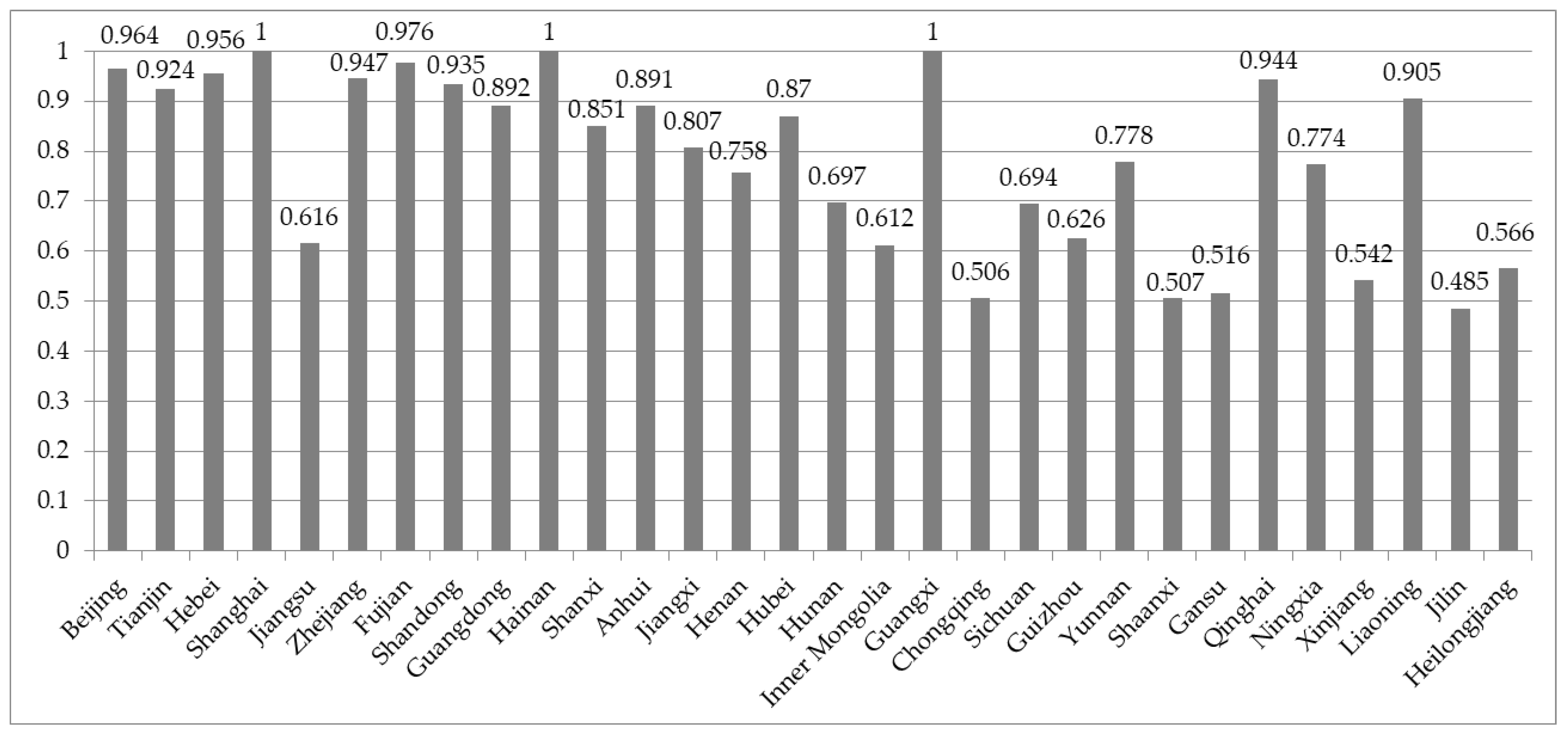
3.1. Efficiency of Fiscal Policies for Environmental Pollution Control
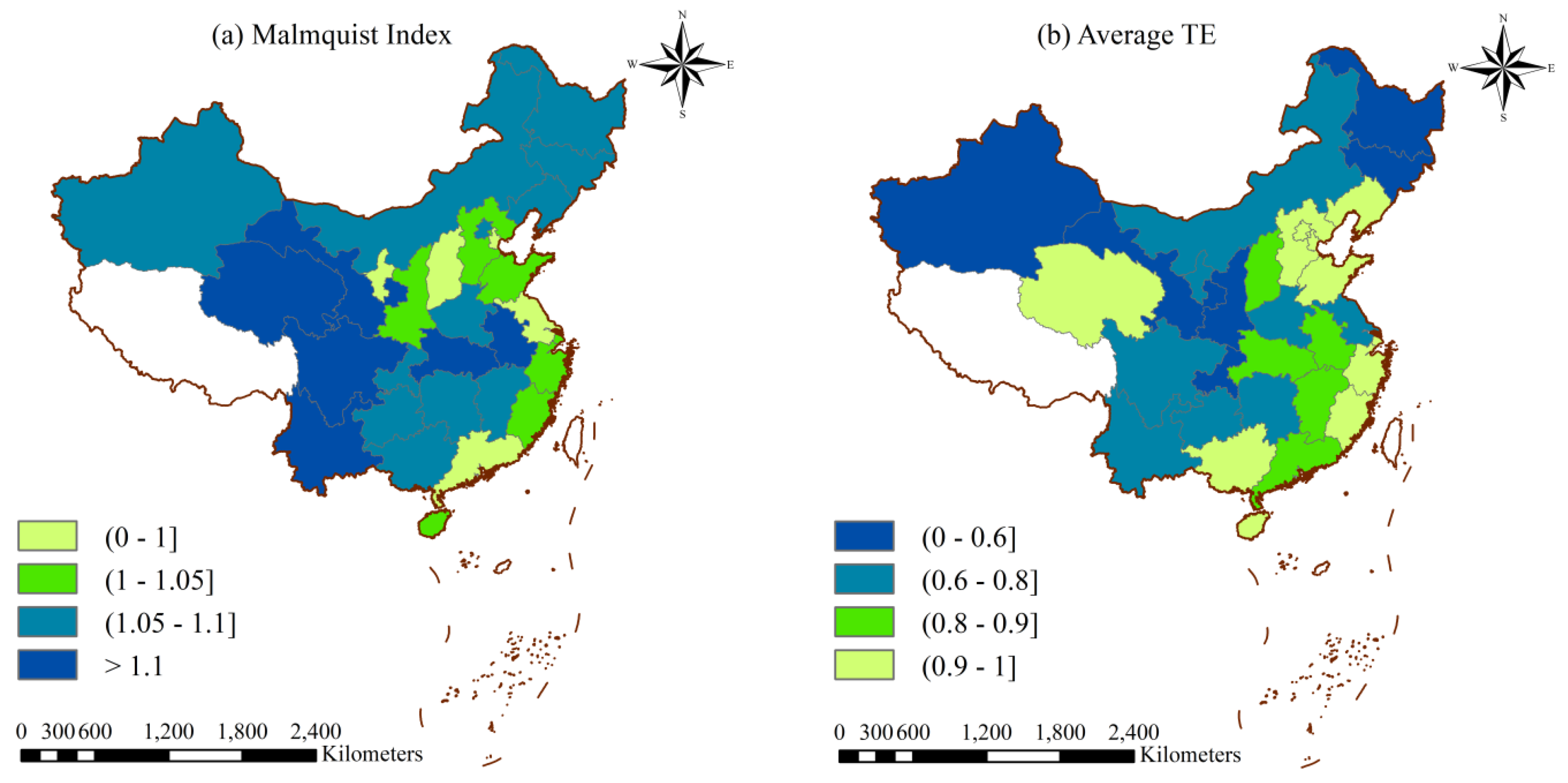
3.2. Malmquist Index and Decomposition Values
3.3. Convergence Analysis
4. The Spatial Effect of Fiscal Decentralization on EFPE
4.1. Index Selection and Data Description
- Explained variable: The technical efficiency (TE) of fiscal policies for environmental pollution control is the explained variable.
- Explanatory variables: To comprehensively measure the impact of fiscal decentralization on environmental fiscal efficiency, fiscal expenditure decentralization (FED) and fiscal revenue decentralization (FRD) are selected as representative indicators of fiscal decentralization [68]. The decentralization of local fiscal expenditure = per capita fiscal expenditure at the local level/(per capita fiscal expenditure at the local level + per capita fiscal expenditure at the central level). The decentralization of local fiscal revenue = per capita local fiscal revenue/(per capita local fiscal revenue + per capita central fiscal revenue).Control variables: To avoid endogeneity problems caused by the omission of variables, the following additional variables that may affect efficiency are selected as control variables. Economic development (ECON) [53] is measured by GDP per capita and deflated by the GDP deflator with 2007 as the base year, and the unit is CNY/person. Population density (POP) [57] is measured by the total population/district area at the end of the year, and the unit is people/. The proportion of industry (IND) [53] is measured by the proportion of industrial added value in GDP, and the unit is %. Energy structure (ENER) [50] is measured by the proportion of coal consumption out of total energy consumption. The relevant proportion is calculated according to the raw coal conversion ratio of 0.7143, and the unit is %. Technical research (TECH) [57] is measured by the annual per capita R&D (research and development) expenditure on R&D personnel; that is, the internal expenditure on R&D divided by R&D personnel is equivalent to full-time equivalent positions. The GDP index based on 2007 is used for the reduction, and the unit is 104 CNY/person.
4.2. Spatial Autocorrelation
4.3. Spatial Econometric Model
4.4. Spatial Effect Analysis
5. Conclusions and Suggestions
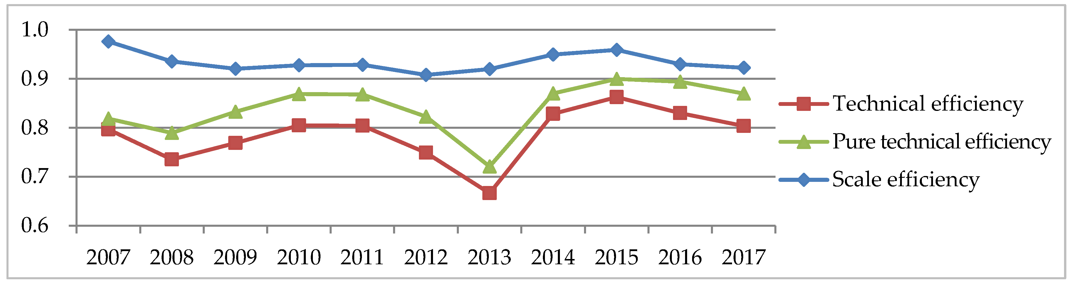
- EFPE has been improved greatly overall since 2014. Although it declined slightly in 2016 and 2017, the level is still high. The change in TE is caused mainly by the change in PTE, while SE is not the main reason for the change in TE. There is regional heterogeneity in EFPE of China. EFPE values in the eastern region are significantly higher than those in other regions. The growth rate of the low efficient region is greater than that of the high efficient region. There is a regional convergence in the EFPE values, and the central region has a relatively fast convergence rate.
- Fiscal expenditure decentralization has a significant direct negative effect and spatial spillover effect on EFPE. Fiscal revenue decentralization has a non-significant impact on EFPE due to fiscal transfer payment. Economic development will still be an important consideration for local governments under current government assessment, and neighboring areas are more likely to compare the economic growth. Economic development has a positive spatial effect and industrial proportion has a negative spatial effect on EFPE.
- The level of fiscal input of environmental governance should be increased, and the central fiscal transfer payment system for environmental protection should be improved. On the basis of the current control of water, soil and air pollution, we should further refine fiscal policies for different pollution types. For example, during the implementation of domestic garbage classification in China, financial support for domestic garbage classification should be increased. We can improve the regulatory role of the central government’s transfer payment policy in environmental governance. Fiscal expenditure for areas with high environmental pressure, heavy tasks and financial pressure increase should be supported to balance the relationship between economic development and environmental protection.
- The government performance assessment system should be reformed, and the conditions of government expenditure on environmental pollution control can be innovated. Government performance assessments should consider not only the scale but also the efficiency of fiscal expenditure on environmental pollution control. The central government may explore setting regional and periodical performance assessment targets for fiscal budgets of environmental governance. Local governments may carry out a whole-process performance evaluation of the pollution control project, and the evaluation subject can be the local government or the third-party institution. By changing the condition of fiscal expenditure, the policy of replacing compensation with reward can be implemented based on the results of pollution control.
- Horizontal fiscal cooperation in cross-regional governance can be promoted to realize regionally coordinated governance. Water pollution, air pollution and other environmental pollution problems have spillover effects among divisions. Therefore, coordination and integration of the fiscal policies should be implemented based on the principle of matching administrative and financial powers in environmental pollution control. By breaking the boundaries of administrative divisions and exploring the horizontal allocation of environmental funds, a cross-domain model of environmental pollution governance can be established. A fiscal expenditure mechanism for environmental protection should be established, so the coordinated regional development can be promoted in China.
Author Contributions
Funding
Acknowledgments
Conflicts of Interest
Appendix A

| Total Amount in Whole Country | Central Government Expenditure | Local Government Expenditure | Proportion of Fiscal Expenditure | Proportion of GDP | |||
|---|---|---|---|---|---|---|---|
| Total Amount | Proportion of Whole Country | Total Amount | Proportion of Whole Country | ||||
| 2007 | 995.82 | 34.59 | 3.47% | 961.24 | 96.53% | 1.94% | 0.37% |
| 2008 | 1451.36 | 66.21 | 4.56% | 1385.15 | 95.44% | 2.37% | 0.45% |
| 2009 | 1934.04 | 37.91 | 1.96% | 1896.13 | 98.04% | 2.82% | 0.55% |
| 2010 | 2441.98 | 69.48 | 2.85% | 2372.50 | 97.15% | 2.94% | 0.59% |
| 2011 | 2640.98 | 74.19 | 2.81% | 2566.79 | 97.19% | 2.54% | 0.54% |
| 2012 | 2963.46 | 63.65 | 2.15% | 2899.81 | 97.85% | 2.53% | 0.55% |
| 2013 | 3435.15 | 100.26 | 2.92% | 3334.89 | 97.08% | 2.66% | 0.58% |
| 2014 | 3815.64 | 344.74 | 9.03% | 3470.90 | 90.97% | 2.72% | 0.59% |
| 2015 | 4802.89 | 400.41 | 8.34% | 4402.48 | 91.66% | 3.15% | 0.70% |
| 2016 | 4734.82 | 295.49 | 6.24% | 4439.33 | 93.76% | 2.52% | 0.65% |
| 2017 | 5617.33 | 350.56 | 6.24% | 5266.77 | 93.76% | 2.76% | 0.72% |
| Indicators | |||||||
|---|---|---|---|---|---|---|---|
| 1 | 0.410 | 0.349 | 0.292 | 0.576 | 0.798 | −0.739 | |
| 0.410 | 1 | 0.287 | 0.488 | 0.522 | 0.789 | −0.672 | |
| 0.349 | 0.287 | 1 | 0.296 | 0.278 | 0.173 | −0.235 | |
| 0.292 | 0.488 | 0.296 | 1 | 0.788 | 0.829 | −0.747 | |
| 0.576 | 0.522 | 0.278 | 0.788 | 1 | 0.761 | −0.808 | |
| 0.798 | 0.789 | 0.173 | 0.829 | 0.761 | 1 | −0.316 | |
| −0.739 | −0.672 | −0.235 | −0.747 | −0.808 | −0.316 | 1 |
| Division | 2007 | 2008 | 2009 | 2010 | 2011 | 2012 | 2013 | 2014 | 2015 | 2016 | 2017 |
|---|---|---|---|---|---|---|---|---|---|---|---|
| Beijing | 1 | 1 | 1 | 1 | 1 | 1 | 1 | 0.972 | 0.897 | 1 | 1 |
| Tianjin | 1 | 1 | 1 | 1 | 1 | 0.966 | 0.808 | 0.812 | 0.939 | 1 | 0.69 |
| Hebei | 1 | 1 | 1 | 1 | 1 | 1 | 1 | 1 | 1 | 1 | 1 |
| Shanghai | 1 | 1 | 1 | 1 | 1 | 1 | 1 | 1 | 1 | 1 | 1 |
| Jiangsu | 1 | 1 | 1 | 1 | 0.965 | 0.908 | 0.896 | 1 | 1 | 1 | 1 |
| Zhejiang | 0.626 | 0.86 | 1 | 1 | 1 | 1 | 1 | 1 | 1 | 1 | 1 |
| Fujian | 1 | 1 | 1 | 1 | 1 | 1 | 1 | 1 | 0.996 | 0.772 | 1 |
| Shandong | 1 | 1 | 1 | 1 | 1 | 1 | 0.711 | 1 | 1 | 1 | 1 |
| Guangdong | 1 | 1 | 1 | 1 | 1 | 1 | 1 | 1 | 1 | 1 | 1 |
| Hainan | 1 | 1 | 1 | 1 | 1 | 1 | 1 | 1 | 1 | 1 | 1 |
| Eastern region | 0.963 | 0.986 | 1.000 | 1.000 | 0.997 | 0.987 | 0.942 | 0.978 | 0.983 | 0.977 | 0.969 |
| Shanxi | 0.714 | 0.873 | 0.804 | 1 | 1 | 1 | 0.526 | 1 | 1 | 1 | 0.952 |
| Anhui | 1 | 1 | 1 | 0.984 | 1 | 1 | 0.562 | 1 | 1 | 1 | 1 |
| Jiangxi | 0.817 | 0.666 | 0.674 | 0.86 | 1 | 0.753 | 0.718 | 1 | 0.949 | 0.98 | 1 |
| Henan | 0.802 | 0.736 | 0.851 | 0.885 | 0.848 | 0.827 | 0.636 | 1 | 0.885 | 0.817 | 0.841 |
| Hubei | 0.962 | 0.847 | 0.894 | 1 | 1 | 0.906 | 0.784 | 1 | 0.942 | 0.862 | 1 |
| Hunan | 0.802 | 0.646 | 0.622 | 0.779 | 0.744 | 0.66 | 0.692 | 0.769 | 1 | 1 | 0.792 |
| Central region | 0.850 | 0.795 | 0.808 | 0.918 | 0.932 | 0.858 | 0.653 | 0.962 | 0.963 | 0.943 | 0.931 |
| Inner Mongolia | 0.972 | 0.64 | 0.651 | 0.682 | 1 | 0.606 | 0.337 | 0.763 | 0.802 | 0.836 | 0.786 |
| Guangxi | 1 | 1 | 1 | 1 | 1 | 1 | 1 | 1 | 1 | 1 | 1 |
| Chongqing | 0.396 | 0.348 | 0.578 | 0.566 | 0.49 | 0.493 | 0.514 | 0.673 | 0.622 | 0.696 | 0.649 |
| Sichuan | 0.923 | 1 | 0.757 | 0.83 | 0.826 | 0.728 | 0.502 | 0.766 | 0.839 | 0.731 | 0.796 |
| Guizhou | 0.487 | 0.528 | 0.533 | 0.663 | 0.727 | 0.745 | 0.759 | 0.814 | 0.871 | 0.53 | 0.55 |
| Yunnan | 0.91 | 0.898 | 1 | 0.923 | 1 | 0.852 | 0.513 | 0.801 | 1 | 0.88 | 0.794 |
| Shaanxi | 0.511 | 0.416 | 0.552 | 0.993 | 0.544 | 0.48 | 0.405 | 0.597 | 0.653 | 0.671 | 0.447 |
| Gansu | 0.501 | 0.37 | 0.412 | 0.512 | 0.391 | 0.462 | 0.39 | 0.53 | 0.54 | 0.945 | 0.914 |
| Qinghai | 1 | 1 | 0.909 | 0.845 | 1 | 1 | 0.806 | 1 | 1 | 1 | 1 |
| Ningxia | 0.532 | 0.538 | 1 | 1 | 0.897 | 0.914 | 0.985 | 1 | 1 | 1 | 0.743 |
| Xinjiang | 0.445 | 0.374 | 0.558 | 0.511 | 0.654 | 0.576 | 0.543 | 0.654 | 0.764 | 0.805 | 1 |
| Western region | 0.698 | 0.647 | 0.723 | 0.775 | 0.775 | 0.714 | 0.614 | 0.782 | 0.826 | 0.827 | 0.789 |
| Liaoning | 0.648 | 0.809 | 0.999 | 1 | 1 | 1 | 0.834 | 1 | 1 | 1 | 1 |
| Jilin | 0.673 | 0.435 | 0.505 | 0.501 | 0.407 | 0.372 | 0.336 | 0.398 | 0.672 | 0.609 | 0.666 |
| Heilongjiang | 0.832 | 0.692 | 0.672 | 0.53 | 0.543 | 0.43 | 0.363 | 0.546 | 0.614 | 0.683 | 0.473 |
| Northeastern region | 0.718 | 0.645 | 0.725 | 0.677 | 0.650 | 0.601 | 0.511 | 0.648 | 0.762 | 0.764 | 0.713 |
| Average of China | 0.818 | 0.789 | 0.832 | 0.869 | 0.868 | 0.823 | 0.721 | 0.870 | 0.900 | 0.894 | 0.870 |
| Division | 2007 | 2008 | 2009 | 2010 | 2011 | 2012 | 2013 | 2014 | 2015 | 2016 | 2017 |
|---|---|---|---|---|---|---|---|---|---|---|---|
| Beijing | 1 | 1 | 1 | 1 | 1 | 1 | 1 | 0.882 | 0.837 | 1 | 1 |
| Tianjin | 1 | 1 | 1 | 1 | 1 | 0.999 | 0.985 | 0.988 | 0.991 | 1 | 0.977 |
| Hebei | 1 | 0.936 | 0.91 | 1 | 1 | 1 | 0.995 | 1 | 0.881 | 0.897 | 0.892 |
| Shanghai | 1 | 1 | 1 | 1 | 1 | 1 | 1 | 1 | 1 | 1 | 1 |
| Jiangsu | 0.632 | 0.541 | 0.588 | 0.885 | 0.641 | 0.675 | 0.676 | 0.676 | 0.654 | 0.684 | 0.775 |
| Zhejiang | 1 | 0.920 | 1 | 1 | 1 | 1 | 1 | 1 | 1 | 1 | 1 |
| Fujian | 1 | 1 | 1 | 1 | 1 | 1 | 0.984 | 1 | 0.996 | 0.979 | 1 |
| Shandong | 1 | 0.945 | 1 | 1 | 1 | 0.842 | 0.793 | 1 | 0.995 | 0.935 | 1 |
| Guangdong | 1 | 1 | 0.957 | 0.72 | 0.76 | 0.687 | 0.732 | 0.959 | 1 | 1 | 1 |
| Hainan | 1 | 1 | 1 | 1 | 1 | 1 | 1 | 1 | 1 | 1 | 1 |
| Eastern region | 0.963 | 0.934 | 0.946 | 0.961 | 0.940 | 0.920 | 0.917 | 0.950 | 0.935 | 0.950 | 0.964 |
| Shanxi | 0.881 | 0.691 | 0.985 | 1 | 1 | 1 | 0.863 | 1 | 1 | 1 | 0.922 |
| Anhui | 1 | 0.986 | 0.984 | 0.856 | 0.879 | 0.748 | 0.984 | 0.985 | 1 | 1 | 0.822 |
| Jiangxi | 1 | 0.980 | 0.997 | 0.984 | 1 | 0.934 | 0.880 | 1 | 0.968 | 0.884 | 0.768 |
| Henan | 0.897 | 0.886 | 0.781 | 0.872 | 0.982 | 0.875 | 0.962 | 0.925 | 1 | 0.976 | 0.894 |
| Hubei | 0.977 | 0.970 | 0.837 | 0.995 | 0.831 | 0.848 | 0.888 | 1 | 0.985 | 0.978 | 1 |
| Hunan | 1 | 0.932 | 0.895 | 0.849 | 0.911 | 0.929 | 0.883 | 0.941 | 0.872 | 0.801 | 0.939 |
| Central region | 0.959 | 0.908 | 0.913 | 0.926 | 0.934 | 0.889 | 0.910 | 0.975 | 0.971 | 0.940 | 0.891 |
| Inner Mongolia | 0.972 | 0.816 | 0.820 | 0.831 | 0.689 | 0.802 | 0.893 | 0.811 | 0.815 | 0.849 | 0.902 |
| Guangxi | 1 | 1 | 1 | 1 | 1 | 1 | 1 | 1 | 1 | 1 | 1 |
| Chongqing | 1 | 0.997 | 0.907 | 0.929 | 0.959 | 0.799 | 0.850 | 0.878 | 0.950 | 0.989 | 0.932 |
| Sichuan | 0.924 | 0.817 | 0.778 | 0.822 | 0.839 | 0.771 | 0.910 | 0.832 | 1 | 0.979 | 0.989 |
| Guizhou | 1 | 0.896 | 0.916 | 0.952 | 0.974 | 0.977 | 0.975 | 0.925 | 0.966 | 0.943 | 0.978 |
| Yunnan | 1 | 0.972 | 0.937 | 0.975 | 0.689 | 0.700 | 0.965 | 0.921 | 1 | 0.826 | 0.877 |
| Shaanxi | 1 | 0.969 | 0.813 | 0.496 | 0.985 | 0.998 | 0.988 | 0.972 | 1 | 0.988 | 0.908 |
| Gansu | 1 | 0.965 | 0.932 | 0.957 | 0.870 | 0.942 | 0.949 | 0.968 | 0.963 | 0.993 | 0.907 |
| Qinghai | 1 | 0.985 | 0.912 | 0.992 | 1 | 1 | 0.906 | 1 | 1 | 1 | 1 |
| Ningxia | 1 | 0.991 | 0.892 | 0.903 | 0.940 | 0.969 | 0.980 | 1 | 1 | 0.528 | 0.583 |
| Xinjiang | 1 | 0.968 | 0.918 | 0.980 | 0.948 | 0.799 | 0.746 | 0.872 | 0.911 | 0.794 | 0.749 |
| Western region | 0.991 | 0.943 | 0.893 | 0.894 | 0.899 | 0.887 | 0.924 | 0.925 | 0.964 | 0.899 | 0.893 |
| Liaoning | 1 | 0.901 | 0.890 | 0.874 | 1 | 1 | 0.982 | 1 | 1 | 1 | 1 |
| Jilin | 1 | 0.995 | 0.974 | 0.956 | 0.961 | 0.954 | 0.952 | 0.980 | 0.999 | 0.913 | 0.862 |
| Heilongjiang | 0.994 | 0.994 | 0.988 | 0.998 | 0.989 | 0.979 | 0.865 | 0.965 | 0.984 | 0.953 | 0.992 |
| Northeastern region | 0.998 | 0.964 | 0.951 | 0.943 | 0.983 | 0.978 | 0.933 | 0.982 | 0.994 | 0.955 | 0.951 |
| Average of China | 0.976 | 0.935 | 0.920 | 0.928 | 0.928 | 0.908 | 0.920 | 0.949 | 0.959 | 0.930 | 0.922 |
References
- Lane, J.E. New Public Management; Routledge: London, UK, 2000. [Google Scholar]
- Li, J. Neo-public Finance: A Paradigm for Enhancing Explanatory and Predictive Power. J. Central. Univ. Finance. Econ. 2017, 5, 3–11. (In Chinese) [Google Scholar]
- The Central Committee of the CPC and the State Council. Opinions on Accelerating the Improvement of the Socialist Market Economy System in the New Era. Available online: http://www.gov.cn/zhengce/2020-05/18/content_5512696.htm (accessed on 18 May 2020).
- Hansen, M.H.; Li, H.; Svarverud, R. Ecological civilization: Interpreting the Chinese past, projecting the global future. Glob. Environ. Chang. 2018, 53, 195–203. [Google Scholar] [CrossRef]
- Frazier, A.E.; Bryan, B.A.; Buyantuev, A.; Chen, L.; Echeverria, C.; Jia, P.; Liu, L.; Li, Q.; Ouyang, Z.; Wu, J.; et al. Ecological civilization: Perspectives from landscape ecology and landscape sustainability science. Landsc. Ecol. 2019, 34, 1–8. [Google Scholar] [CrossRef]
- Jiang, B.; Bai, Y.; Wong, C.P.; Xu, X.; Alatalo, J.M. China’s ecological civilization program–Implementing ecological redline policy. Land Use Policy 2019, 81, 111–114. [Google Scholar] [CrossRef]
- Zhou, C.; Wang, P.; Zhang, X. Does Fiscal Policy Promote Third-Party Environmental Pollution Control in China? An Evolutionary Game Theoretical Approach. Sustainability 2019, 11, 4434. [Google Scholar] [CrossRef]
- China Ministry of Finance. Finance Yearbook of China; China Financial Magazine: Beijing, China, 2008–2018. [Google Scholar]
- Gu, C. The Track Change and Evolution Characteristics of Fiscal Decentralization in China. Res. Chin. Econ. Hist. 2009, 2, 43–51. (In Chinese) [Google Scholar]
- Veld, K.V.T.; Shogren, J.F. Environmental federalism and environmental liability. J. Environ. Econ. Manag. 2012, 63, 105–119. [Google Scholar] [CrossRef]
- Zhang, N.; Deng, J.; Ahmad, F.; Draz, M.U. Local Government Competition and Regional Green Development in China: The Mediating Role of Environmental Regulation. Int. J. Environ. Res. Public Health 2020, 17, 3485. [Google Scholar] [CrossRef]
- López, N.R.; García, J.M.; Uribe-Toril, J.; Valenciano, J.D.P. Evolution and latest trends of local government efficiency: Worldwide research (1928–2019). J. Clean. Prod. 2020, 261, 121276. [Google Scholar] [CrossRef]
- Zhang, Z.; Zhang, G.; Song, S.; Su, B. Spatial Heterogeneity Influences of Environmental Control and Informal Regulation on Air Pollutant Emissions in China. Int. J. Environ. Res. Public Health 2020, 17, 4857. [Google Scholar] [CrossRef]
- Peng, Y. Investment Behavior of Local Government, the Level of Economic Development and Carbon Emissions: An Empirical Analysis Based on Chinese Provincial Panel Data. Comp. Econ. Soc. Syst. 2013, 3, 92–99. (In Chinese) [Google Scholar]
- Tang, E.; Liu, F.; Zhang, J.; Yu, J. A model to analyze the environmental policy of resource reallocation and pollution control based on firms’ heterogeneity. Resour. Policy 2014, 39, 88–91. [Google Scholar] [CrossRef]
- Tian, S.; Dong, W.; Xu, W. Environmental Fiscal Expenditure, Government Environmental Preference and Policy Effect: An Empirical Analysis Based on Inter-provincial Industrial Pollution Data. Inq. Econ. Issues 2016, 7, 14–21. (In Chinese) [Google Scholar]
- Halkos, G.E.; Paizanos, E.A. The effect of government expenditure on the environment:An empirical investigation. Ecol. Econ. 2013, 91, 48–56. [Google Scholar] [CrossRef]
- Zhang, Q.; Zhang, S.; Ding, Z.; Hao, Y. Does government expenditure affect environmental quality? Empirical evidence using Chinese city-level data. J. Clean. Prod. 2017, 161, 143–152. [Google Scholar] [CrossRef]
- Pearce, D. The Role of Carbon Taxes in Adjusting to Global Warming. Econ. J. 1991, 101, 938. [Google Scholar] [CrossRef]
- Wissema, W.; Dellink, R. AGE analysis of the impact of a carbon energy tax on the Irish economy. Ecol. Econ. 2007, 61, 671–683. [Google Scholar] [CrossRef]
- Glomm, G.; Kawaguchi, D.; Sepulveda, F. Green taxes and double dividends in a dynamic economy. J. Policy Model. 2008, 30, 19–32. [Google Scholar] [CrossRef]
- Piciu, G.C.; Trică, C.L. Assessing the Impact and Effectiveness of Environmental Taxes. Procedia Econ. Financ. 2012, 3, 728–733. [Google Scholar] [CrossRef]
- Li, G.; Masui, T. Assessing the impacts of China’s environmental tax using a dynamic computable general equilibrium model. J. Clean. Prod. 2019, 208, 316–324. [Google Scholar] [CrossRef]
- Xiong, B.; Chen, W.; Liu, P.; Xu, W. Fiscal Policy, Local Governments Competition and Air Pollution Control Quality. J. China Univ. Geosci. (Soc. Sci.) 2016, 1, 20–33, 170. (In Chinese) [Google Scholar]
- Zhu, X.; Lu, Y. Pollution governance effect on environmental fiscal and taxation policy: Based on region and threshold effect. China Popul. Resour. Environ. 2017, 1, 83–90. (In Chinese) [Google Scholar]
- Yang, Z. China’s Public Finance from 1978 to 2018: Ideas and Changes. Financ. Trade Econ. 2018, 10, 5–16. (In Chinese) [Google Scholar]
- Emrouznejad, A.; Yang, G.-L. A survey and analysis of the first 40 years of scholarly literature in DEA: 1978–2016. Socio-Econ. Plan. Sci. 2018, 61, 4–8. [Google Scholar] [CrossRef]
- Wang, M.; Gilmour, S.; Tao, C.; Zhuang, K. Does Scale and Efficiency of Government Health Expenditure Promote Development of the Health Industry? Int. J. Environ. Res. Public Health 2020, 17, 5529. [Google Scholar] [CrossRef]
- Özbuğday, F.C.; Tirgil, A.; Kose, E.G. Efficiency changes in long-term care in OECD countries: A non-parametric Malmquist Index approach. Socio-Econ. Plan. Sci. 2020, 70, 100733. [Google Scholar] [CrossRef]
- Chen, M.; Pei, X. A Study of the Efficiency of China’s Financial Policy for Environmental Governance: Based on DEA Cross Evaluation. Contemp. Financ. Econ. 2013, 4, 27–36. (In Chinese) [Google Scholar]
- Meng, F.; Fan, L.; Zhou, P.; Zhou, D. Measuring environmental performance in China’s industrial sectors with non-radial DEA. Math. Comput. Model. 2013, 58, 1047–1056. [Google Scholar] [CrossRef]
- Zhu, H.; Fu, Q.; Wei, Q. Calculation of Efficiency on Environmental Expenditure and Study on Influential Factor. China Popul. Resour. Environ. 2014, 6, 91–96. (In Chinese) [Google Scholar]
- Jin, R.; Zhang, D. Research on the Efficiency of Environmental Protection Expenditures by Provincial Governments in China. J. Bus. Manag. 2012, 11, 152–159. (In Chinese) [Google Scholar]
- Liu, B.; Wang, B.; Xue, G. On Assessment of Public Spending Efficiency of Environment Protection in Local China: Based on Three-stage Bootstrapped DEA. J. Zhongnan Univ. Econ. Law 2016, 1, 89–95. (In Chinese) [Google Scholar]
- Fare, R.; Grosskopf, S.; Norris, M.; Zhang, Z. Productivity Growth, Technical Progress, and Efficiency Changes in Industrialized Countries. Am. Econ. Rev. 1994, 1, 66–84. [Google Scholar]
- An, Q.; Wu, Q.; Li, J.; Xiong, B.; Chen, X. Environmental efficiency evaluation for Xiangjiang River basin cities based on an improved SBM model and Global Malmquist index. Energy Econ. 2019, 81, 95–103. [Google Scholar] [CrossRef]
- Sun, C. Performance Evaluation on Energy Policies in Beijing-Tianjin-Hebei Region under Background of Regional Integration. Technol. Econ. 2016, 6, 91–95. (In Chinese) [Google Scholar]
- Fan, S.; Chen, Y.; Xu, J. Performance Evaluation and Comparison of Ecological Construction Policies Based on Public Value. J. Public Manag. 2013, 2, 110–116. (In Chinese) [Google Scholar]
- Li, W. Analysis of the Efficiency and Evaluation of Chinese Industrial Pollution Control Policy and Advices for Environmental Policy. Sci. Technol. Manag. Res. 2014, 17, 20–26. (In Chinese) [Google Scholar]
- Huang, R.; Zhao, Q. Performance Evaluation of China’s Environmental Protection Financial Funds (2006–2011) Based on Content Analysis of Audit Results Announcement. Public Financ. Res. 2012, 5, 31–35. (In Chinese) [Google Scholar]
- Wang, K.; Wang, J.; Hubacek, K.; Mi, Z.; Wei, Y. A cost–benefit analysis of the environmental taxation policy in China: A frontier analysis-based environmentally extended input–output optimization method. J. Ind. Ecol. 2020, 24, 564–576. [Google Scholar] [CrossRef]
- Narbón-Perpiñá, I.; Arribas, I.; Balaguer-Coll, M.T.; Tortosa-Ausina, E. Explaining local governments’ cost efficiency: Controllable and uncontrollable factors. Cities 2020, 100, 102665. [Google Scholar] [CrossRef]
- Zhang, K.; Wang, J.; Cui, X. Fiscal Decentralization and Environmental Pollution: From the Perspective of Carbon Emission. China Ind. Econ. 2011, 12, 65–75. (In Chinese) [Google Scholar]
- Huang, S. A Study of Impacts of Fiscal Decentralization on Smog Pollution. J. World Econ. 2017, 2, 127–152. (In Chinese) [Google Scholar]
- Wu, H.; Hao, Y.; Ren, S. How do environmental regulation and environmental decentralization affect green total factor energy efficiency: Evidence from China. Energy Econ. 2020, 91, 104880. [Google Scholar] [CrossRef]
- Chen, S.; Song, Y.; Ding, Y.; Qian, X.; Zhang, M. Research on the strategic interaction and convergence of China’s environmental public expenditure from the perspective of inequality. Resour. Conserv. Recycl. 2019, 145, 19–30. [Google Scholar] [CrossRef]
- Pan, X.; Li, M.; Guo, S.; Pu, C. Research on the competitive effect of local government’s environmental expenditure in China. Sci. Total. Environ. 2020, 718, 137238. [Google Scholar] [CrossRef] [PubMed]
- Wu, H.; Li, Y.; Hao, Y.; Ren, S.; Zhang, P. Environmental decentralization, local government competition, and regional green development: Evidence from China. Sci. Total. Environ. 2020, 708, 135085. [Google Scholar] [CrossRef]
- Liu, Q. Fiscal Decentralization, Governmental Incentives and Environmental Pollution Abatement. Econ. Survey 2013, 2, 127–132. (In Chinese) [Google Scholar]
- Han, J.; Meng, D. An Empirical Analysis on Spatial Effects of Fiscal Decentralization on Ecological Environment: Evidence from Provincial Panel Data. Public Financ. Res. 2018, 3, 71–77. (In Chinese) [Google Scholar]
- Zheng, J.; Fu, C.; Zhang, C. Fiscal Decentralization and Environmental Pollution: From the Perspective of New Structural Economics. Public Financ. Res. 2018, 3, 57–70. (In Chinese) [Google Scholar]
- Kuai, P.; Yang, S.; Tao, A.; Zhang, S.; Khan, Z.D. Environmental effects of Chinese-style fiscal decentralization and the sustainability implications. J. Clean. Prod. 2019, 239, 118089. [Google Scholar] [CrossRef]
- Li, X.; Liu, H. Fiscal Decentralization and the Plight of Regional Environmental Pollution Based on the Perspective of Regional Differences: The Analysis on the Pollutant Properties of Spillover. Financ. Trade Econ. 2016, 2, 41–54. (In Chinese) [Google Scholar]
- He, Q. Fiscal decentralization and environmental pollution: Evidence from Chinese panel data. China Econ. Rev. 2015, 36, 86–100. [Google Scholar] [CrossRef]
- Fu, Y. Fiscal Decentralization, Governance and Non-Economic Public Goods Provision. J. Econ. Res. 2010, 8, 4–15. (In Chinese) [Google Scholar]
- Pan, X. Efficiency Analysis of China’s Local Government’s Expenditure on Environmental Protection. China Popul. Resour. Environ. 2013, 11, 61–65. (In Chinese) [Google Scholar]
- Zhang, X.; Yuan, H.; Hao, F. Fiscal decentralization influence on environmental investment efficiency: Analysis based on DEA-Tobit model. China Environ. Sci. 2018, 12, 4780–4787. (In Chinese) [Google Scholar]
- Lin, C.; Sun, Y. The Relationship between Fiscal Decentralization and China’s Environmental Governance Performance: Empirical Test Based on Provincial Panel Data. Reform Econ. Syst. 2019, 2, 150–155. (In Chinese) [Google Scholar]
- Charnes, A.; Cooper, W.W.; Rhodes, E. Measuring the Efficiency of Decision Making Unites. Eur. J. Oper. Res. 1978, 2, 429–444. [Google Scholar] [CrossRef]
- Banker, R.D.; Charnes, A.; Cooper, W.W. Some Models for Estimating Technical and Scale Inefficiencies in Data Envelopment Analysis. Manag. Sci. 1984, 30, 1078–1092. [Google Scholar] [CrossRef]
- National Bureau of Statistics of China. China Statistical Yearbook; China Statistical Press: Beijing, China, 2008–2018. [Google Scholar]
- Ministry of Environmental Protection and National Bureau of Statistics of China. China Statistical Yearbook on Environment; China Statistical Press: Beijing, China, 2008–2018. [Google Scholar]
- Ministry of Environmental Protection of China. China Environment Yearbook; China Environmental Yearbook Press: Beijing, China, 2008–2018. [Google Scholar]
- The Central Committee of the CPC and the State Council. Several Opinions on Promoting the Rise of the Central Region. Available online: http://www.gov.cn/zhengce/content/2012-08/31/content_1147.htm (accessed on 20 September 2020).
- The State Council of China. Several Opinions of on the Implementation of Policies and Measures for the Large-scale Development of the Western Region. Available online: http://www.gov.cn/gongbao/content/2001/content_61158.htm (accessed on 20 September 2020).
- Tan, J. Correlation Analysis in Evaluation Index System. Stat. Decis. 2005, 22, 147–148. (In Chinese) [Google Scholar]
- Barro, R.; Sala-i-Martin, X. Convergence. J. Polit. Econ. 1992, 100, 223–251. [Google Scholar] [CrossRef]
- Gong, F.; Lei, X. The Quantitive Measurement of Chinese-style fiscal decentralization. Stat. Res. 2010, 10, 47–55. (In Chinese) [Google Scholar]
- National Bureau of Statistics of China. China Regional Economic Statistical Yearbook; China Statistical Press: Beijing, China, 2008–2018. [Google Scholar]
- Department of Energy Statistics, National Bureau of Statistics of China. China Energy Statistical Yearbook; China Statistical Press: Beijing, China, 2008–2018. [Google Scholar]
- National Bureau of Statistics of China. China High-Tech Industry Statistical Yearbook; China Statistical Press: Beijing, China, 2008–2018. [Google Scholar]


| Variable | Classification | Indicator | Definition of Indicator |
|---|---|---|---|
| Inputs | Fiscal expenditure policy | Fiscal expenditure of environmental protection-pollutant discharge fee | Environmental fiscal expenditure excluding pollutant discharge fee |
| Fiscal revenue policy | Pollutant discharge fee | Pollutant discharge fee collected by local governments | |
| Outputs | Pollution treatment of wastewater | Sanitary wastewater treatment | Sewage treatment capacity of municipal sewage treatment plants [34] |
| Industrial wastewater treatment | Discharge and treatment capacity of industrial wastewater | ||
| Pollution treatment of solid waste | Domestic garbage treatment | The amount of harmless disposal of urban household waste [34] | |
| Industrial solid waste treatment | Amount of comprehensive utilization of industrial solid waste [33] | ||
| Pollution treatment of waste gas | Treatment effect of | Ratio of emissions/ 104 CNY of GDP in the base period and emissions/104 CNY of GDP in the current year |
| Division | 2007 | 2008 | 2009 | 2010 | 2011 | 2012 | 2013 | 2014 | 2015 | 2016 | 2017 |
|---|---|---|---|---|---|---|---|---|---|---|---|
| Beijing | 1 | 1 | 1 | 1 | 1 | 1 | 1 | 0.857 | 0.751 | 1 | 1 |
| Tianjin | 1 | 1 | 1 | 1 | 1 | 0.965 | 0.796 | 0.802 | 0.931 | 1 | 0.674 |
| Hebei | 1 | 0.936 | 0.91 | 1 | 1 | 1 | 0.995 | 1 | 0.881 | 0.897 | 0.892 |
| Shanghai | 1 | 1 | 1 | 1 | 1 | 1 | 1 | 1 | 1 | 1 | 1 |
| Jiangsu | 0.632 | 0.541 | 0.588 | 0.885 | 0.619 | 0.613 | 0.606 | 0.676 | 0.654 | 0.684 | 0.775 |
| Zhejiang | 0.626 | 0.791 | 1 | 1 | 1 | 1 | 1 | 1 | 1 | 1 | 1 |
| Fujian | 1 | 1 | 1 | 1 | 1 | 1 | 0.984 | 1 | 0.992 | 0.756 | 1 |
| Shandong | 1 | 0.945 | 1 | 1 | 1 | 0.842 | 0.564 | 1 | 0.995 | 0.935 | 1 |
| Guangdong | 1 | 1 | 0.957 | 0.72 | 0.76 | 0.687 | 0.732 | 0.959 | 1 | 1 | 1 |
| Hainan | 1 | 1 | 1 | 1 | 1 | 1 | 1 | 1 | 1 | 1 | 1 |
| Eastern region | 0.926 | 0.921 | 0.946 | 0.961 | 0.938 | 0.911 | 0.868 | 0.929 | 0.920 | 0.927 | 0.934 |
| Shanxi | 0.629 | 0.603 | 0.792 | 1 | 1 | 1 | 0.454 | 1 | 1 | 1 | 0.878 |
| Anhui | 1 | 0.986 | 0.984 | 0.842 | 0.879 | 0.748 | 0.553 | 0.985 | 1 | 1 | 0.822 |
| Jiangxi | 0.817 | 0.653 | 0.672 | 0.846 | 1 | 0.703 | 0.632 | 1 | 0.919 | 0.866 | 0.768 |
| Henan | 0.719 | 0.652 | 0.665 | 0.772 | 0.833 | 0.724 | 0.612 | 0.925 | 0.885 | 0.797 | 0.752 |
| Hubei | 0.94 | 0.822 | 0.748 | 0.995 | 0.831 | 0.768 | 0.696 | 1 | 0.928 | 0.843 | 1 |
| Hunan | 0.802 | 0.602 | 0.557 | 0.661 | 0.678 | 0.613 | 0.611 | 0.724 | 0.872 | 0.801 | 0.744 |
| Central region | 0.818 | 0.720 | 0.736 | 0.853 | 0.870 | 0.759 | 0.593 | 0.939 | 0.934 | 0.885 | 0.827 |
| Inner Mongolia | 0.945 | 0.522 | 0.534 | 0.567 | 0.689 | 0.486 | 0.301 | 0.619 | 0.654 | 0.71 | 0.709 |
| Guangxi | 1 | 1 | 1 | 1 | 1 | 1 | 1 | 1 | 1 | 1 | 1 |
| Chongqing | 0.396 | 0.347 | 0.524 | 0.526 | 0.47 | 0.394 | 0.437 | 0.591 | 0.591 | 0.688 | 0.605 |
| Sichuan | 0.853 | 0.817 | 0.589 | 0.682 | 0.693 | 0.561 | 0.457 | 0.637 | 0.839 | 0.716 | 0.787 |
| Guizhou | 0.487 | 0.473 | 0.488 | 0.631 | 0.708 | 0.728 | 0.74 | 0.753 | 0.841 | 0.5 | 0.538 |
| Yunnan | 0.91 | 0.873 | 0.937 | 0.9 | 0.689 | 0.596 | 0.495 | 0.738 | 1 | 0.727 | 0.696 |
| Shaanxi | 0.511 | 0.403 | 0.449 | 0.493 | 0.536 | 0.479 | 0.4 | 0.58 | 0.653 | 0.663 | 0.406 |
| Gansu | 0.501 | 0.357 | 0.384 | 0.49 | 0.34 | 0.435 | 0.37 | 0.513 | 0.52 | 0.938 | 0.829 |
| Qinghai | 1 | 0.985 | 0.829 | 0.838 | 1 | 1 | 0.73 | 1 | 1 | 1 | 1 |
| Ningxia | 0.532 | 0.533 | 0.892 | 0.903 | 0.843 | 0.886 | 0.965 | 1 | 1 | 0.528 | 0.433 |
| Xinjiang | 0.445 | 0.362 | 0.512 | 0.501 | 0.62 | 0.46 | 0.405 | 0.57 | 0.696 | 0.639 | 0.749 |
| Western region | 0.689 | 0.607 | 0.649 | 0.685 | 0.690 | 0.639 | 0.573 | 0.727 | 0.799 | 0.737 | 0.705 |
| Liaoning | 0.648 | 0.729 | 0.889 | 0.874 | 1 | 1 | 0.819 | 1 | 1 | 1 | 1 |
| Jilin | 0.673 | 0.433 | 0.492 | 0.479 | 0.391 | 0.355 | 0.32 | 0.39 | 0.671 | 0.556 | 0.574 |
| Heilongjiang | 0.827 | 0.688 | 0.664 | 0.529 | 0.537 | 0.421 | 0.314 | 0.527 | 0.604 | 0.651 | 0.469 |
| Northeastern region | 0.716 | 0.617 | 0.682 | 0.627 | 0.643 | 0.592 | 0.484 | 0.639 | 0.758 | 0.736 | 0.681 |
| Average of China | 0.796 | 0.735 | 0.769 | 0.804 | 0.804 | 0.749 | 0.666 | 0.828 | 0.863 | 0.830 | 0.803 |
| Index | EFFCH | PECH | SECH | TECHCH | Malmquist Index | |
|---|---|---|---|---|---|---|
| Division | ||||||
| Beijing | 1 | 1 | 1 | 1.071 | 1.071 | |
| Tianjin | 0.961 | 0.964 | 0.998 | 0.988 | 0.949 | |
| Hebei | 0.989 | 1 | 0.989 | 1.061 | 1.049 | |
| Shanghai | 1 | 1 | 1 | 1.014 | 1.014 | |
| Jiangsu | 1.021 | 1 | 1.021 | 0.957 | 0.977 | |
| Zhejiang | 1.048 | 1.048 | 1 | 0.955 | 1.001 | |
| Fujian | 1 | 1 | 1 | 1.011 | 1.011 | |
| Shandong | 1 | 1 | 1 | 1.016 | 1.016 | |
| Guangdong | 1 | 1 | 1 | 0.974 | 0.974 | |
| Hainan | 1 | 1 | 1 | 1.049 | 1.049 | |
| Eastern region | 1.002 | 1.001 | 1.001 | 1.010 | 1.011 | |
| Shanxi | 1.034 | 1.029 | 1.005 | 0.945 | 0.977 | |
| Anhui | 0.981 | 1 | 0.981 | 1.141 | 1.119 | |
| Jiangxi | 0.994 | 1.02 | 0.974 | 1.059 | 1.052 | |
| Henan | 1.005 | 1.005 | 1 | 1.069 | 1.073 | |
| Hubei | 1.006 | 1.004 | 1.002 | 1.121 | 1.128 | |
| Hunan | 0.993 | 0.999 | 0.994 | 1.07 | 1.062 | |
| Central region | 1.002 | 1.01 | 0.993 | 1.068 | 1.069 | |
| Inner Mongolia | 0.972 | 0.979 | 0.993 | 1.091 | 1.06 | |
| Guangxi | 1 | 1 | 1 | 1.07 | 1.07 | |
| Chongqing | 1.043 | 1.051 | 0.993 | 1.045 | 1.091 | |
| Sichuan | 0.992 | 0.985 | 1.007 | 1.11 | 1.101 | |
| Guizhou | 1.01 | 1.012 | 0.998 | 1.088 | 1.099 | |
| Yunnan | 0.974 | 0.987 | 0.987 | 1.196 | 1.165 | |
| Shaanxi | 0.977 | 0.987 | 0.991 | 1.071 | 1.047 | |
| Gansu | 1.052 | 1.062 | 0.99 | 1.159 | 1.218 | |
| Qinghai | 1 | 1 | 1 | 1.129 | 1.129 | |
| Ningxia | 0.98 | 1.034 | 0.947 | 1.003 | 0.982 | |
| Xinjiang | 1.053 | 1.084 | 0.971 | 1.029 | 1.084 | |
| Western region | 1.005 | 1.016 | 0.989 | 1.090 | 1.095 | |
| Liaoning | 1.044 | 1.044 | 1 | 1.034 | 1.08 | |
| Jilin | 0.984 | 0.999 | 0.985 | 1.077 | 1.06 | |
| Heilongjiang | 0.945 | 0.945 | 1 | 1.145 | 1.081 | |
| Northeast region | 0.991 | 0.996 | 0.995 | 1.085 | 1.074 | |
| Average of China | 1.002 | 1.008 | 0.994 | 1.056 | 1.058 | |
| Region | Whole Country | Eastern Region | Central Region | Western Region | Northeastern Region | |
|---|---|---|---|---|---|---|
| Coefficient | ||||||
| 0.99 | 0.99 | 0.99 | 0.99 | 0.90 | ||
| p value of | 0 | 0 | 0 | 0 | 0.04 | |
| 0.08 | 0.09 | 0.13 | 0.08 | 0.32 | ||
| p value of | 0 | 0.02 | 0.01 | 0.01 | 0.31 | |
| R squared adjusted | 0.53 | 0.44 | 0.86 | 0.52 | 0.56 | |
| Index | 2007 | 2008 | 2009 | 2010 | 2011 | 2012 | 2013 | 2014 | 2015 | 2016 | 2017 |
|---|---|---|---|---|---|---|---|---|---|---|---|
| I value | 0.118 | 0.277 | 0.28 | 0.324 | 0.213 | 0.172 | 0.284 | 0.234 | 0.127 | 0.13 | 0.202 |
| Z value | 1.663 | 2.59 | 2.617 | 3.025 | 2.15 | 1.704 | 2.696 | 2.324 | 1.784 | 1.854 | 1.941 |
| p value | 0.03 | 0.009 | 0.005 | 0.002 | 0.028 | 0.041 | 0.014 | 0.017 | 0.043 | 0.035 | 0.033 |
| Variable | Direct Effect | Indirect Effect | Total Effect | |
|---|---|---|---|---|
| Explanatory variables | FED | −1.547 ** (−2.16) | −1.079 * (−1.84) | −2.625 ** (−2.09) |
| FRD | −0.060 (−0.26) | −0.042 (−0.26) | −0.102 (−0.26) | |
| Control variables | ECON | 0.513 ** (2.53) | 0.358 ** (2.05) | 0.871 ** (2.42) |
| POP | −0.379 (−1.21) | −0.264 (−1.15) | −0.643 (−1.20) | |
| IND | −0.541 *** (−3.11) | −0.377 ** (−2.48) | −0.918 *** (−3.02) | |
| ENER | 0.105 (0.97) | 0.073 (0.91) | 0.178 (0.95) | |
| TECH | 0.013 (0.36) | 0.009 (0.36) | 0.023 (0.36) |
Publisher’s Note: MDPI stays neutral with regard to jurisdictional claims in published maps and institutional affiliations. |
© 2020 by the authors. Licensee MDPI, Basel, Switzerland. This article is an open access article distributed under the terms and conditions of the Creative Commons Attribution (CC BY) license (http://creativecommons.org/licenses/by/4.0/).
Share and Cite
Zhou, C.; Zhang, X. Measuring the Efficiency of Fiscal Policies for Environmental Pollution Control and the Spatial Effect of Fiscal Decentralization in China. Int. J. Environ. Res. Public Health 2020, 17, 8974. https://doi.org/10.3390/ijerph17238974
Zhou C, Zhang X. Measuring the Efficiency of Fiscal Policies for Environmental Pollution Control and the Spatial Effect of Fiscal Decentralization in China. International Journal of Environmental Research and Public Health. 2020; 17(23):8974. https://doi.org/10.3390/ijerph17238974
Chicago/Turabian StyleZhou, Caihua, and Xinmin Zhang. 2020. "Measuring the Efficiency of Fiscal Policies for Environmental Pollution Control and the Spatial Effect of Fiscal Decentralization in China" International Journal of Environmental Research and Public Health 17, no. 23: 8974. https://doi.org/10.3390/ijerph17238974
APA StyleZhou, C., & Zhang, X. (2020). Measuring the Efficiency of Fiscal Policies for Environmental Pollution Control and the Spatial Effect of Fiscal Decentralization in China. International Journal of Environmental Research and Public Health, 17(23), 8974. https://doi.org/10.3390/ijerph17238974