Geographic Inequalities of Respiratory Health Services Utilization during Childhood in Edmonton and Calgary, Canada: A Tale of Two Cities

 , ,
, , 
Abstract
1. Introduction
2. Materials and Methods
2.1. Study Design and Setting
2.2. Study Population
2.3. Definition of Geographic Areas
2.4. Explanatory Variable: Spatial Filters
2.5. Study Outcome
Smoothed Standardized Prevalence Ratios (SPR) of Respiratory Health Services Utilization
2.6. Covariates
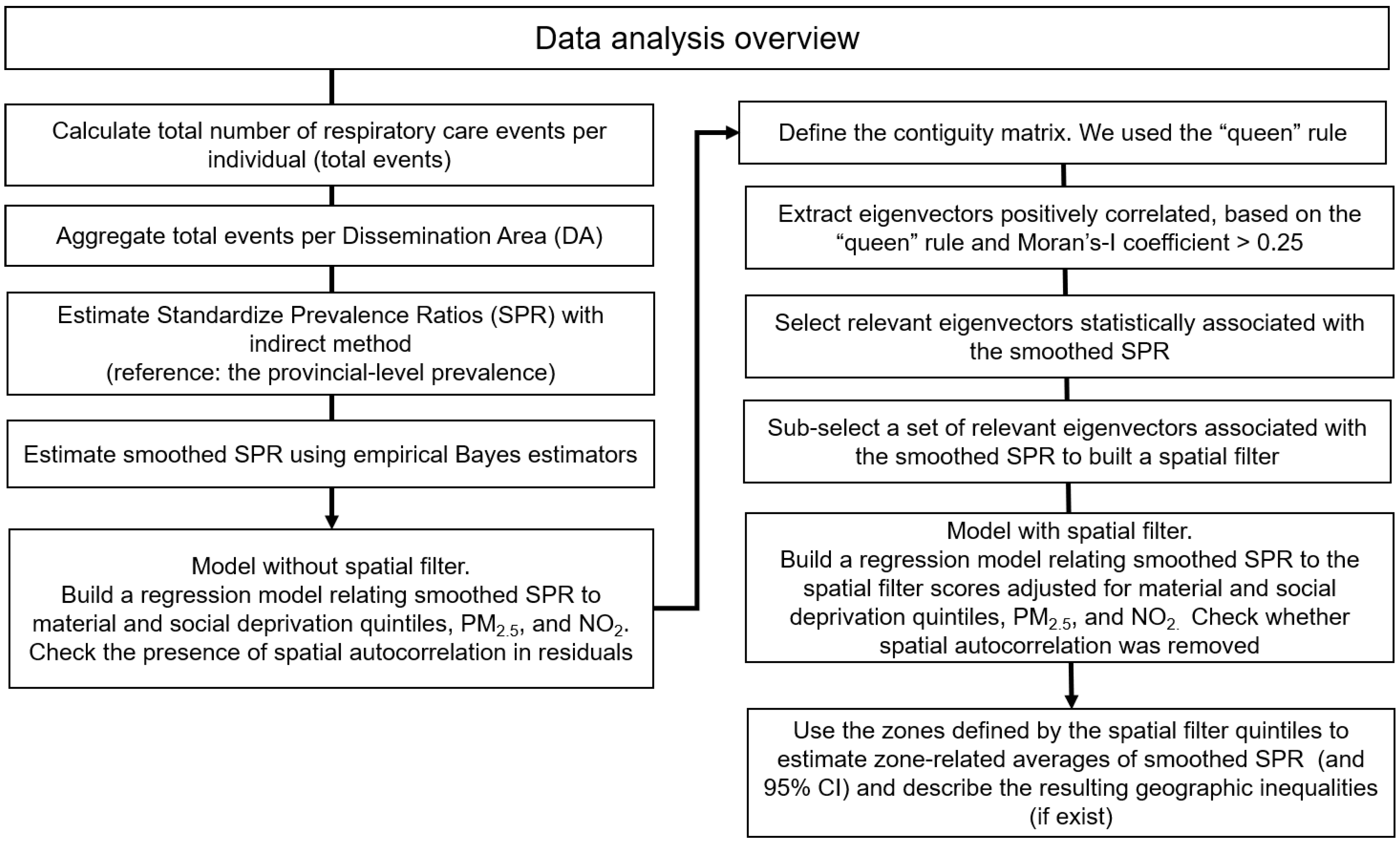
2.7. Data Analysis
3. Results
3.1. Descriptive Statistics
3.2. Calgary
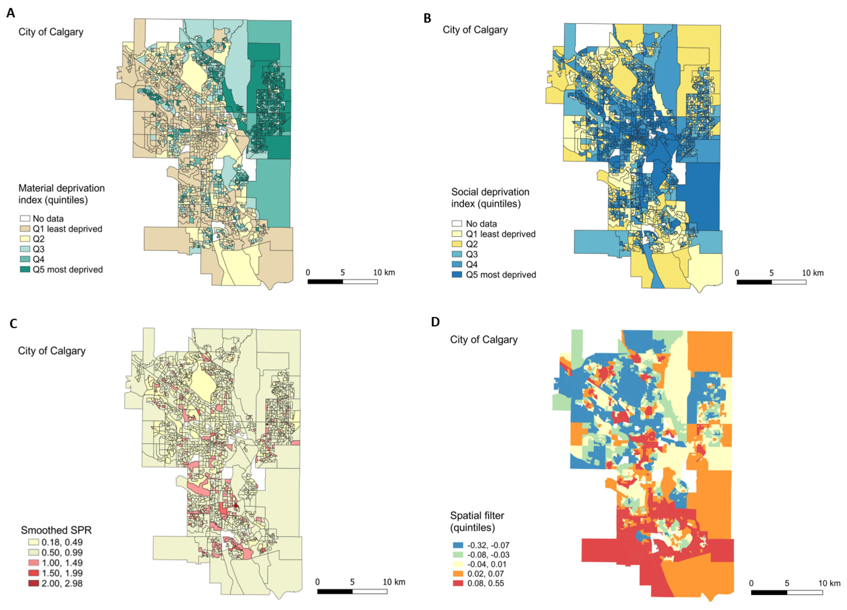
3.2.1. Exploratory Maps
3.2.2. Regression Models for Smoothed-SPR without and with Spatial Filter
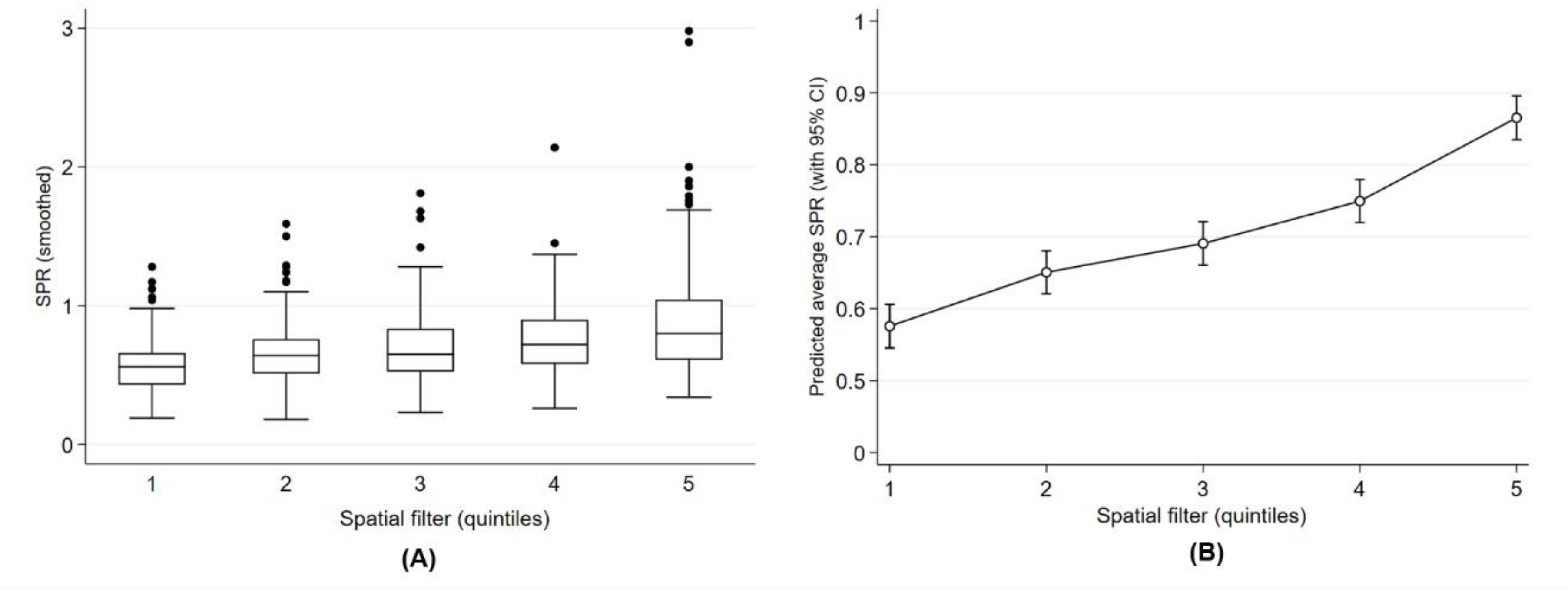
3.2.3. Geographic Inequality
3.3. Edmonton
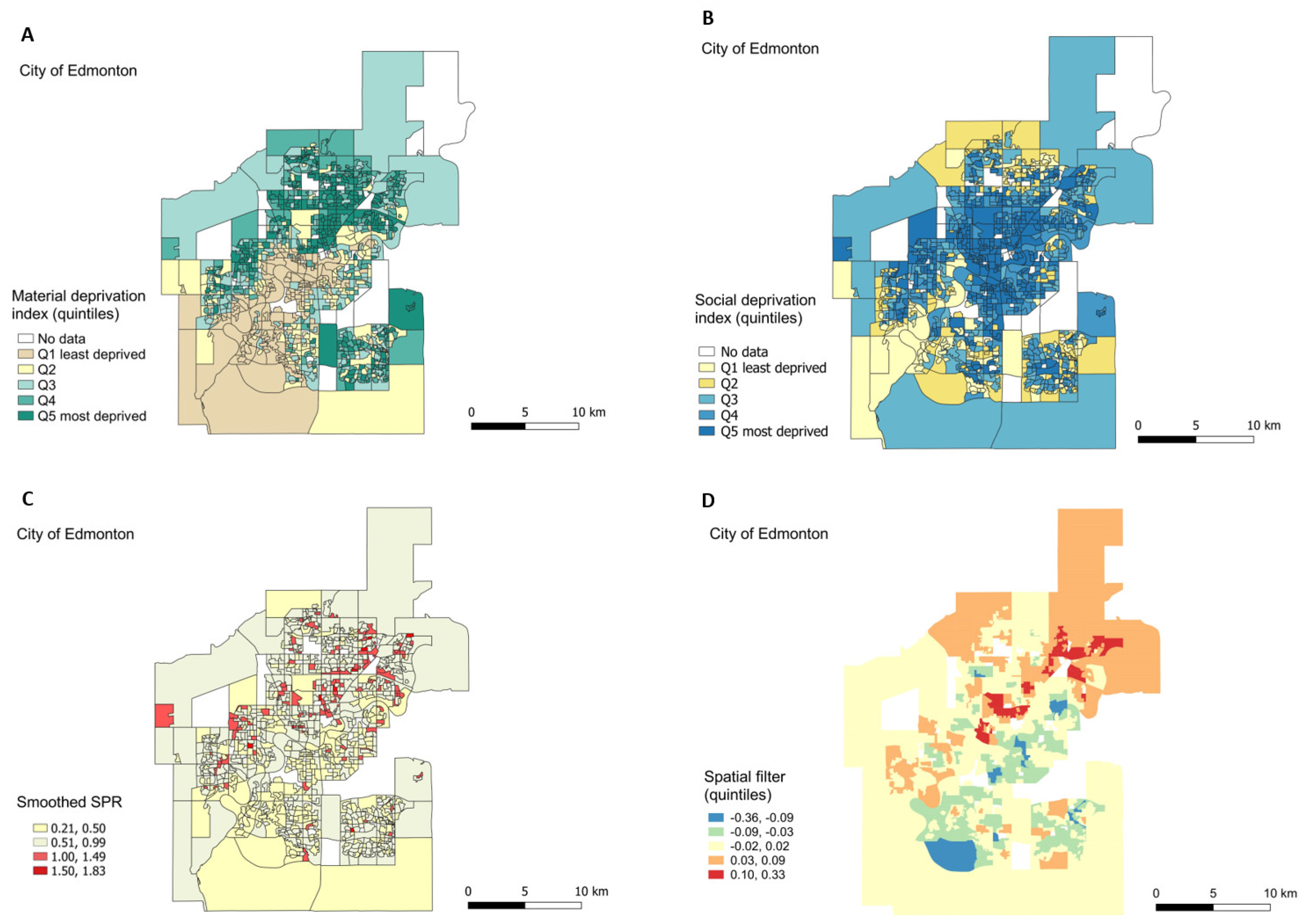
3.3.1. Exploratory Maps
3.3.2. Regression Models for Smoothed-SPR without and with Spatial Filter
3.3.3. Geographic Inequality
4. Discussion
Strengths and Limitations
5. Conclusions
Supplementary Materials
Author Contributions
Funding
Acknowledgments
Conflicts of Interest
References
- Zar, H.J.; Ferkol, T.W. The global burden of respiratory disease-impact on child health. Pediatr. Pulmonol. 2014, 49, 430–434. [Google Scholar] [CrossRef] [PubMed]
- Wang, H.; Naghavi, M.; Allen, C.; Bhutta, Z.A.; Carter, A.; Casey, D.C.; Charlson, F.J.; Chen, A.Z.; Coates, M.M.; Coggeshall, M. Global, regional, and national life expectancy, all-cause mortality, and cause-specific mortality for 249 causes of death, 1980–2015: A systematic analysis for the global burden of disease study 2015. Lancet 2016, 388, 1459–1544. [Google Scholar] [CrossRef]
- Belgrave, D.C.M.; Buchan, I.; Bishop, C.; Lowe, L.; Simpson, A.; Custovic, A. Trajectories of lung function during childhood. Am. J. Respir. Crit. Care Med. 2014, 189, 1101–1109. [Google Scholar] [CrossRef] [PubMed]
- Lancet Respiratory Medicine. Health inequality: A major driver of respiratory disease. Lancet Resp. Med. 2017, 5, 235. [CrossRef]
- Foley, D.; Best, E.; Reid, N.; Berry, M. Respiratory health inequality starts early: The impact of social determinants on the aetiology and severity of bronchiolitis in infancy. J. Paediatr. Child Health 2019, 55, 528–532. [Google Scholar] [CrossRef] [PubMed]
- Uphoff, E.; Cabieses, B.; Pinart, M.; Valdés, M.; Antó, J.M.; Wright, J. A systematic review of socioeconomic position in relation to asthma and allergic diseases. Eur. Respir. J. 2015, 46, 364–374. [Google Scholar] [CrossRef]
- Williams, D.R.; Sternthal, M.; Wright, R.J. Social determinants: Taking the social context of asthma seriously. Pediatrics 2009, 123, S174–S184. [Google Scholar] [CrossRef]
- Raphael, D. The health of Canada’s children. Part II: Health mechanisms and pathways. Paediatr. Child Health 2010, 15, 71–76. [Google Scholar] [CrossRef][Green Version]
- Raphael, D. The health of Canada’s children. Part III: Public policy and the social determinants of children’s health. Paediatr. Child Health 2010, 15, 143–149. [Google Scholar] [CrossRef]
- Corsi, D.J.; Boyle, M.H.; Lear, S.A.; Chow, C.K.; Teo, K.K.; Subramanian, S.V. Trends in smoking in Canada from 1950 to 2011: Progression of the tobacco epidemic according to socioeconomic status and geography. Cancer Causes Control 2014, 25, 45–57. [Google Scholar] [CrossRef]
- Ospina, M.B.; Voaklander, D.; Senthilselvan, A.; Stickland, M.K.; King, M.; Harris, A.W.; Rowe, B.H. Incidence and prevalence of chronic obstructive pulmonary disease among Aboriginal Peoples in Alberta, Canada. PLoS ONE 2015, 10, e0123204. [Google Scholar] [CrossRef] [PubMed]
- Ospina, M.B.; Rowe, B.H.; Voaklander, D.; Sentilselvan, A.; Stickland, M.K.; King, M. Emergency department visits after diagnosed chronic obstructive pulmonary disease in Aboriginal People in Alberta, Canada. CJEM 2016, 18, 420–428. [Google Scholar] [CrossRef] [PubMed]
- Canadian Institute for Health Information. Trends in Income-Related Health Inequalities in Canada: Summary Report; Canadian Institute for Health Information: Ottawa, ON, Canada, 2015; Available online: https://www.cihi.ca/sites/default/files/document/summary_report_inequalities_2015_en.pdf (accessed on 17 June 2020).
- Canadian Institute for Health Information. Asthma Hospitalizations among Children and Youth in Canada: Trends and Inequalities; Canadian Institute for Health Information: Ottawa, ON, Canada, 2018; Available online: https://www.cihi.ca/sites/default/files/document/asthma-hospitalization-children-2018-chartbook-en-web.pdf (accessed on 9 September 2020).
- Rosychuk, R.J.; Youngson, E.; Rowe, B.H. Presentations to Alberta emergency departments for asthma: A time series analysis. Acad. Emerg. Med. 2015, 22, 942–949. [Google Scholar] [CrossRef] [PubMed]
- Kovesi, T. Respiratory disease in Canadian First Nations and Inuit children. Paediatr. Child Health 2012, 17, 376–380. [Google Scholar] [CrossRef] [PubMed][Green Version]
- Morrison, K.T.; Buckeridge, D.L.; Xiao, Y.; Moghadas, S.M. The impact of geographical location of residence on disease outcomes among Canadian First Nations populations during the 2.009 influenza A(H1N1) pandemic. Health Place 2014, 26, 53–59. [Google Scholar] [CrossRef] [PubMed]
- Belon, A.P.; Serrano-Lomelin, J.; Nykiforuk, C.I.J.; Hicks, A.; Crawford, S.; Bakal, J.; Ospina, M.B. Health gradients in emergency visits and hospitalisations for paediatric respiratory diseases: A population-based retrospective cohort study. Paediatr. Perinat. Epidemiol. 2020, 4, 150–160. [Google Scholar] [CrossRef] [PubMed]
- Agrawal, S. Urban, Suburban, Regional and Wet Growth in Alberta. University of Alberta. 2016. Available online: https://www.albertalandinstitute.ca/public/download/documents/34087 (accessed on 9 September 2016).
- Smyth, F. Medical geography: Understanding health inequalities. Prog. Hum. Geogr. 2008, 32, 119–127. [Google Scholar] [CrossRef]
- Shawky, S. Measuring geographic and wealth inequalities in health distribution as tools for identifying priority health inequalities and the underprivileged populations. Glob. Adv. Health Med. 2018, 7, 1–10. [Google Scholar] [CrossRef]
- Smith, S.J.; Easterlow, D. The strange geography of health inequalities. Trans. Inst. Br. Geog. 2005, 30, 173–190. [Google Scholar] [CrossRef]
- Von Elm, E.; Altman, D.G.; Egger, M.; Pocock, S.J.; Gøtzsche, P.C.; Vandenbroucke, J.P. The strengthening the reporting of observational studies in epidemiology (STROBE) statement: Guidelines for reporting observational studies. Bull. World Health Organ. 2007, 85, 867–872. [Google Scholar] [CrossRef]
- Government of Alberta. Alberta Population Estimates. 2020. Available online: https://www.alberta.ca/population-statistics.aspx#population-estimates (accessed on 17 August 2017).
- City of Calgary. Past Census Results. 2020. Available online: https://www.calgary.ca/ca/city-clerks/election-and-information-services/civic-census/censusresults.html (accessed on 17 August 2020).
- Edmonton City Government. Municipal Census Results. 2019. Available online: https://www.edmonton.ca/city_government/facts_figures/municipal-census-results.aspx (accessed on 17 August 2020).
- Canadian Institute for Health Information. ICD-10-CA. International Statistical Classification of Diseases and Related Health Problems; Canadian Institute for Health Information: Ottawa, ON, Canada, 2015; Available online: https://www.cihi.ca/sites/default/files/icd_volume_one_2015_en_0.pdf (accessed on 2 October 2016).
- Statistics Canada. Dissemination Area: Detailed Definition. 2018. Available online: https://www150.statcan.gc.ca/n1/pub/92-195-x/2011001/geo/da-ad/def-eng.htm (accessed on 22 June 2020).
- DMTI Spatial Inc. Platinum Postal Suite: CanMap Multiple Enhanced Postal Code Geography 2001–2013; Computer File; DMTI Spatial Inc.: Markham, ON, Canada, 2014. [Google Scholar]
- Statistics Canada. GeoSuite, 2006. Census Geographic Data Products; Statistics Canada Catalogue No. 92F0150XCB; Statistics Canada: Ottawa, ON, Canada, 2007. [Google Scholar]
- Statistics Canada. Census—Boundary Files: Reference Guide. Statistics Canada Catalogue No. gda_000b06a_e.zip. 2007. Available online: http://www12.statcan.ca/census-recensement/2011/geo/bound-limit/bound-limit-2006-eng.cfm (accessed on 5 June 2015).
- Griffith, D.A. Spatial Autocorrelation and Spatial Filtering: Gaining Understanding through Theory and Scientific Visualization; Springer Science & Business Media: Berlin, Germany, 2003. [Google Scholar]
- Tiefelsdorf, M.; Griffith, D.A. Semiparametric filtering of spatial autocorrelation: The eigenvector approach. Section A (Economy and Space). Environ. Plan. 2007, 39, 1193–1221. [Google Scholar] [CrossRef]
- Griffith, D.A.; Chun, Y.; Li, B. Spatial Regression Analysis Using Eigenvector Spatial Filtering; E-Book; Academic Press: San Diego, CA, USA, 2019. [Google Scholar] [CrossRef]
- Patuelli, R.; Griffith, D.A.; Tiefelsdorf, M.; Nijkamp, P. The Use of Spatial Filtering Techniques: The Spatial and Space-Time Structure of German Unemployment Data. Tinbergen Institute Discussion Papers, No 06-049/3, Tinbergen Institute. 2006. Available online: https://econpapers.repec.org/paper/tinwpaper/20060049.htm (accessed on 22 June 2020).
- Griffith, D.; Chun, Y. Spatial autocorrelation and spatial filtering. In Handbook of Regional Science; Fischer, M.M., Nijkamp, P., Eds.; Springer: Berlin/Heidelberg, Germany, 2014; pp. 1477–1507. [Google Scholar] [CrossRef]
- Chen, Y. New approaches for calculating Moran’s Index of spatial autocorrelation. PLoS ONE 2013, 8, e68336. [Google Scholar] [CrossRef] [PubMed]
- Marshall, R.J. Mapping disease and mortality rates using empirical Bayes estimators. J. R. Stat. Soc. 1991, 40, 283–294. [Google Scholar] [CrossRef]
- Rabe-Hesketh, S.; Skrondal, A. Multilevel and Longitudinal Modeling Using Stata, 2nd ed.; Stata Press: College Station, TX, USA, 2008. [Google Scholar]
- Stata Statistical Software, version 15.1; StataCorp: College Station, TX, USA, 2017.
- Pampalon, R.; Hamel, D.; Gamache, P.; Philibert, M.D.; Raymond, G.; Simpson, A. Un indice régional de défavorisation matérielle et sociale pour la santé publique au Québec et au Canada. Can. J. Public Health 2012, 103, S17–S22. [Google Scholar] [CrossRef] [PubMed]
- Pampalon, R.; Hamel, D.; Gamache, P.; Raymond, G. A deprivation index for health planning in Canada. Chronic Dis. Can. 2009, 29, 178–191. [Google Scholar] [CrossRef] [PubMed]
- Gamache, P.; Hamel, D.; Blaser, C. Material and Social Deprivation Index: A Summary. Institut National de Santé Publique du Québec, Bureau D’information et D’études en Santé des Populations—INSPQ Website. 2019. Available online: www.inspq.qc.ca/en/publications/2639 (accessed on 9 September 2020).
- Hystad, P.; Setton, E.; Cervantes, A.; Poplawski, K.; Deschenes, S.; Brauer, M.; van Donkelaar, A.; Lamsal, L.; Martin, R.; Jerrett, M.; et al. Creating national air pollution models for population exposure assessment in Canada. Environ. Health Perspect. 2011, 119, 1123–1129. [Google Scholar] [CrossRef]
- ArcGIS Desktop versión 10.5; Esri Inc.: Redlands, CA, USA, 2016.
- QGIS version 3.4.14. QGIS org: A Free and Open Source Geographic Information System. 2019. Available online: https://www.qgis.org/en/site/ (accessed on 17 January 2020).
- Townshend, I.; Miller, B.; Evans, L. Socio-Spatial Polarization in an Age of Income Inequality: An Exploration of Neighbourhood Change in Calgary’s “Three Cities”. 2018. Available online: http://neighbourhoodchange.ca/documents/2018/04/socio-spatial-polarization-in-calgary.pdf (accessed on 22 June 2020).
- City of Edmonton. Recovery Program. What We Did. GIS Mapping. 2020. Available online: https://www.urbanwellnessedmonton.com/gis-mapping-detail (accessed on 17 June 2020).
- Beamer, P.I.; Lothrop, N.; Lu, Z.; Ascher, R.; Ernst, K.; Stern, D.A.; Billheimer, D.; Wright, A.L.; Martinez, F.D. Spatial clusters of child lower respiratory illnesses associated with community-level risk factors: Risk factors for childhood LRI clusters. Pediatr. Pulmonol. 2016, 51, 633–642. [Google Scholar] [CrossRef]
- Diette, G.B.; McCormack, M.C.; Hansel, N.N.; Breysse, P.N.; Matsui, E.C. Environmental issues in managing asthma. Respir. Care 2008, 53, 602–617. [Google Scholar]
- Legerski, E.M.; Thayn, J.B. The effects of spatial patterns of neighborhood risk factors on adverse birth outcomes. Soc. Sci. J. 2013, 50, 635–645. [Google Scholar] [CrossRef]
- Sierra-Heredia, C.; North, M.; Brook, J.; Daly, C.; Ellis, A.; Henderson, D.; Henderson, S.B.; Lavigne, É.; Takaro, T.K. Aeroallergens in Canada: Distribution, public health impacts, and opportunities for prevention. Int. J. Environ. Res. Public Health 2018, 15, 1577. [Google Scholar] [CrossRef]
- Dales, R.E.; Cakmak, S.; Judek, S.; Dann, T.; Coates, F.; Brook, J.R.; Burnett, R.T. Influence of outdoor aeroallergens on hospitalization for asthma in Canada. J. Allergy Clin. Immunol. 2004, 113, 303–306. [Google Scholar] [CrossRef] [PubMed]
- Sibley, L.M.; Weiner, J.P. An evaluation of access to health care services along the rural-urban continuum in Canada. BMC Health Serv. Res. 2011, 11, 1–20. [Google Scholar] [CrossRef] [PubMed]
- Cutchin, M.P.; Eschbach, K.; Mair, C.A.; Ju, H.; Goodwin, J.S. The socio-spatial neighborhood estimation method: An approach to operationalizing the neighborhood concept. Health Place 2011, 17, 1113–1121. [Google Scholar] [CrossRef] [PubMed]
- Nielsen, C.C.; Amrhein, C.G.; Shah, P.S.; Aziz, K.; Osornio-Vargas, A.R. Spatiotemporal patterns of small for gestational age and low birth weight births and associations with land use and socioeconomic status. Environ. Health Insights 2019, 13, 1–13. [Google Scholar] [CrossRef] [PubMed]
- Borrell, C.; Marí-Dell’Olmo, M.; Serral, G.; Martínez-Beneito, M.; Gotsens, M. Inequalities in mortality in small areas of eleven Spanish cities (the multicenter MEDEA project). Health Place 2010, 16, 703–711. [Google Scholar] [CrossRef]
- Nielsen, C.C.; Amrhein, C.G.; Shah, P.S.; Stieb, D.M.; Osornio-Vargas, A.R. Space-time hot spots of critically ill small for gestational age newborns and industrial air pollutants in major metropolitan areas of Canada. Environ. Res. 2020, 186, 109472. [Google Scholar] [CrossRef]
- Oyana, T.J.; Podila, P.; Wesley, J.M.; Lomnicki, S.; Cormier, S. Spatiotemporal patterns of childhood asthma hospitalization and utilization in Memphis Metropolitan Area from 2005 to 2015. J. Asthma 2017, 54, 842–855. [Google Scholar] [CrossRef]
- Skrivankova, V.; Zwahlen, M.; Adams, M.; Low, N.; Kuehni, C.; Egger, M. Spatial epidemiology of gestational age and birth weight in Switzerland: Census-based linkage study. BMJ Open 2019, 9, 1–11. [Google Scholar] [CrossRef]
- Yu, D.; Zhang, Y.; Wu, X. How socioeconomic and environmental factors impact the migration destination choices of different population groups in China: An eigenfunction-based spatial filtering analysis. Popul. Environ. 2020, 41, 372–395. [Google Scholar] [CrossRef]
- Diniz-Filho, J.A.F.; Bini, L.M. Modelling geographical patterns in species richness using eigenvector-based spatial filters. Glob. Ecol. Biogeogr. 2005, 14, 177–185. [Google Scholar] [CrossRef]
- Griffith, D.A.; Peres-Neto, P.R. Spatial modeling in ecology: The flexibility of eigenfunction spatial analyses. Ecology 2006, 87, 2603–2613. [Google Scholar] [CrossRef]
- Jerrett, M.; Gale, S.; Kontgis, C. Spatial modeling in environmental and public health research. Int. J. Environ. Res. Public Health 2010, 7, 1302–1329. [Google Scholar] [CrossRef] [PubMed]
- Canada Post. Addressing Guidelines, Effective January 31, 2019, Section 5.3 Local Delivery Unit—The Second Segment of the Postal Code. 2019. Available online: https://www.canadapost.ca/tools/pg/manual/pgaddress-e.asp (accessed on 20 June 2020).
- Bell, M.L.; Banerjee, G.; Pereira, G. Residential mobility of pregnant women and implications for assessment of spatially-varying environmental exposures. J. Expo. Sci. Environ. Epidemiol. 2018, 28, 470–480. [Google Scholar] [CrossRef] [PubMed]
- Chen, L.; Bell, E.M.; Caton, A.R.; Druschel, C.M.; Lin, S. Residential mobility during pregnancy and the potential for ambient air pollution exposure misclassification. Environ. Res. 2010, 110, 162–168. [Google Scholar] [CrossRef] [PubMed]


| Calgary | Edmonton | |||
|---|---|---|---|---|
| N | % | N | % | |
| Births | 70,862 | 100 | 49,047 | 100 |
| Material deprivation quintiles | ||||
| Q1 (least deprived) | 24,313 | 34 | 8908 | 18 |
| Q2 | 13,256 | 19 | 6681 | 14 |
| Q3 | 10,675 | 15 | 9667 | 20 |
| Q4 | 7619 | 11 | 11,347 | 23 |
| Q5 (most deprived) | 14,110 | 20 | 10,945 | 22 |
| missing | 889 | 1 | 1499 | 3 |
| Social deprivation quintiles | ||||
| Q1 (least deprived) | 9682 | 14 | 4107 | 8 |
| Q2 | 16,569 | 23 | 9257 | 19 |
| Q3 | 15,266 | 22 | 10,243 | 21 |
| Q4 | 13,094 | 18 | 9865 | 20 |
| Q5 (most deprived) | 15,362 | 22 | 14,076 | 29 |
| missing | 889 | 1 | 1499 | 3 |
| Number of Dissemination Areas (DA) | 1431 | 1090 | ||
| Model A (without Spatial Filter) | Model B (with Spatial Filter) | |||||
|---|---|---|---|---|---|---|
| Independent Variables | Coefficient | p-Value | 95% CI | Coefficient | p-Value | 95% CI |
| Spatial filter | NA | 0.99 | 0.000 | [0.87, 1.12] | ||
| Material quintiles | ||||||
| Q1 (least deprived) | Reference | Reference | ||||
| Q2 | 0.06 | 0.009 | [0.01, 0.10] | 0.04 | 0.033 | [0.00, 0.08] |
| Q3 | 0.05 | 0.039 | [0.00, 0.09] | 0.05 | 0.023 | [0.01, 0.09] |
| Q4 | 0.01 | 0.723 | [−0.04, 0.05] | 0.01 | 0.700 | [−0.03, 0.05] |
| Q5 (most deprived) | 0.05 | 0.016 | [0.01, 0.09] | 0.07 | 0.000 | [0.04, 0.11] |
| Social quintiles | ||||||
| Q1 (least deprived) | Reference | Reference | ||||
| Q2 | 0.02 | 0.519 | [−0.03, 0.07] | 0.02 | 0.414 | [−0.03, 0.06] |
| Q3 | 0.02 | 0.502 | [−0.03, 0.06] | 0.03 | 0.173 | [−0.01, 0.07] |
| Q4 | 0.02 | 0.336 | [−0.02, 0.07] | 0.04 | 0.047 | [0.00, 0.09] |
| Q5 (most deprived) | 0.09 | 0.000 | [0.05, 0.14] | 0.09 | 0.000 | [0.05, 0.13] |
| PM2.5 | 0.09 | 0.002 | [0.03, 0.14] | 0.01 | 0.599 | [−0.04, 0.07] |
| NO2 | 0.00 | 0.079 | [−0.01, 0.00] | 0.00 | 0.891 | [0.00, 0.01] |
| constant | 0.13 | 0.506 | [−0.24, 0.50] | 0.53 | 0.002 | [0.19, 0.88] |
| Adjusted R-squared = 0.02 | Adjusted R-squared = 0.17 | |||||
| AIC = 333.36 | AIC = 103.04 | |||||
| BIC = 391.07 | BIC = 166.00 | |||||
| Moran’s-I of residuals: 0.048, p-value < 0.01 | Moran’s-I of residuals: −0.033, p-value = 0.63 | |||||
| Model A (without Spatial Filter) | Model B (with Spatial Filter) | |||||
|---|---|---|---|---|---|---|
| Independent Variables | Coefficient | p-Value | 95% CI | Coefficient | p-Value | 95% CI |
| Spatial filter | NA | 0.98 | 0.000 | [0.81, 1.15] | ||
| Material | ||||||
| Q1 (least deprived) | Reference | Reference | ||||
| Q2 | 0.09 | 0.001 | [0.04, 0.15] | 0.06 | 0.024 | [0.01, 0.11] |
| Q3 | 0.10 | 0.000 | [0.05, 0.15] | 0.06 | 0.021 | [0.01, 0.11] |
| Q4 | 0.19 | 0.000 | [0.14, 0.24] | 0.12 | 0.000 | [0.07, 0.17] |
| Q5 (most deprived) | 0.22 | 0.000 | [0.18, 0.27] | 0.15 | 0.000 | [0.10, 0.20] |
| Social | ||||||
| Q1 (least deprived) | Reference | Reference | ||||
| Q2 | 0.04 | 0.157 | [−0.02, 0.10] | 0.05 | 0.063 | [−0.01, 0.11] |
| Q3 | 0.05 | 0.080 | [−0.01, 0.11] | 0.05 | 0.133 | [−0.01, 0.10] |
| Q4 | 0.09 | 0.001 | [0.04, 0.15] | 0.10 | 0.000 | [0.05, 0.15] |
| Q5 (most deprived) | 0.18 | 0.000 | [0.13, 0.23] | 0.18 | 0.000 | [0.13, 0.23] |
| PM2.5 | 0.01 | 0.458 | [−0.01, 0.03] | 0.01 | 0.905 | [−0.02, 0.02] |
| NO2 | 0.00 | 0.113 | [−0.01, 0.00] | 0.00 | 0.168 | [−0.01, 0.00] |
| Constant | 0.47 | 0.000 | [0.30, 0.64] | 0.55 | 0.000 | [0.38, 0.71] |
| Adjusted R-squared = 0.14 | Adjusted R-squared = 0.23 | |||||
| AIC = 74.70 | AIC = -46.64 | |||||
| BIC = 129.08 | BIC = 12.68 | |||||
| Moran’s-I of residuals: 0.046, p-value < 0.01 | Moran’s-I of residuals: −0.017, p-value = 0.67 | |||||
Publisher’s Note: MDPI stays neutral with regard to jurisdictional claims in published maps and institutional affiliations. |
© 2020 by the authors. Licensee MDPI, Basel, Switzerland. This article is an open access article distributed under the terms and conditions of the Creative Commons Attribution (CC BY) license (http://creativecommons.org/licenses/by/4.0/).
Share and Cite
Serrano-Lomelin, J.; Nielsen, C.C.; Hicks, A.; Crawford, S.; Bakal, J.A.; Ospina, M.B. Geographic Inequalities of Respiratory Health Services Utilization during Childhood in Edmonton and Calgary, Canada: A Tale of Two Cities. Int. J. Environ. Res. Public Health 2020, 17, 8973. https://doi.org/10.3390/ijerph17238973
Serrano-Lomelin J, Nielsen CC, Hicks A, Crawford S, Bakal JA, Ospina MB. Geographic Inequalities of Respiratory Health Services Utilization during Childhood in Edmonton and Calgary, Canada: A Tale of Two Cities. International Journal of Environmental Research and Public Health. 2020; 17(23):8973. https://doi.org/10.3390/ijerph17238973
Chicago/Turabian StyleSerrano-Lomelin, Jesus, Charlene C. Nielsen, Anne Hicks, Susan Crawford, Jeffrey A. Bakal, and Maria B. Ospina. 2020. "Geographic Inequalities of Respiratory Health Services Utilization during Childhood in Edmonton and Calgary, Canada: A Tale of Two Cities" International Journal of Environmental Research and Public Health 17, no. 23: 8973. https://doi.org/10.3390/ijerph17238973
APA StyleSerrano-Lomelin, J., Nielsen, C. C., Hicks, A., Crawford, S., Bakal, J. A., & Ospina, M. B. (2020). Geographic Inequalities of Respiratory Health Services Utilization during Childhood in Edmonton and Calgary, Canada: A Tale of Two Cities. International Journal of Environmental Research and Public Health, 17(23), 8973. https://doi.org/10.3390/ijerph17238973