Ecological Engineering for the Optimisation of the Land-Based Marine Aquaculture of Coastal Shellfish


Abstract
1. Introduction
2. Material and Methods
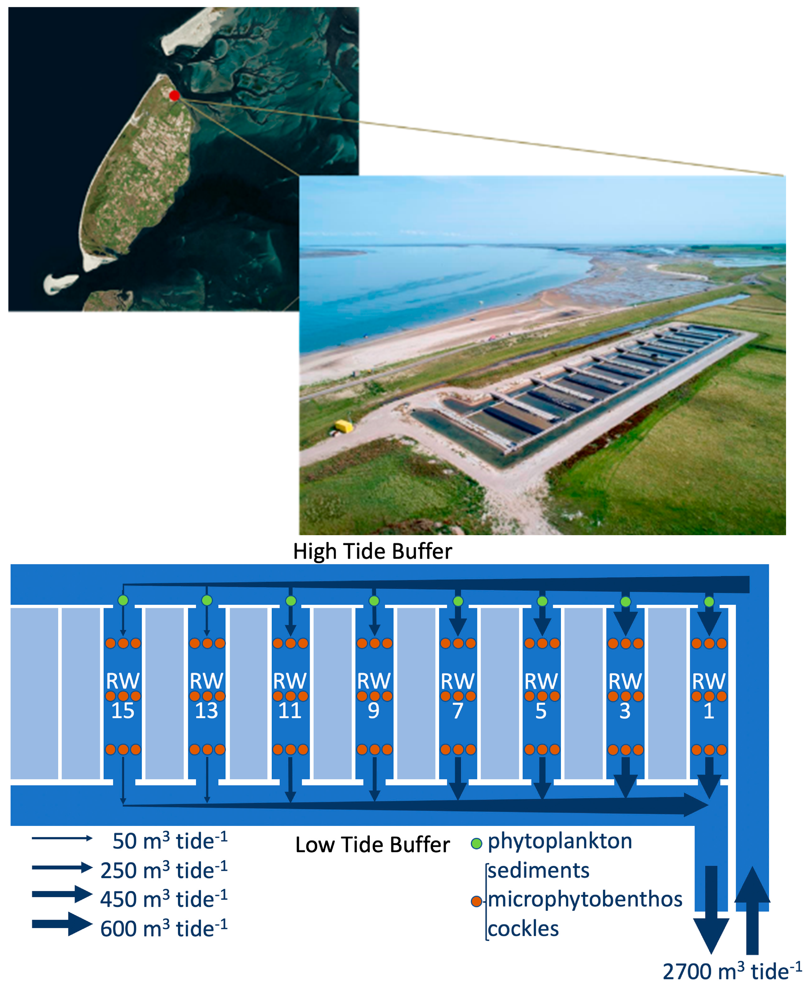
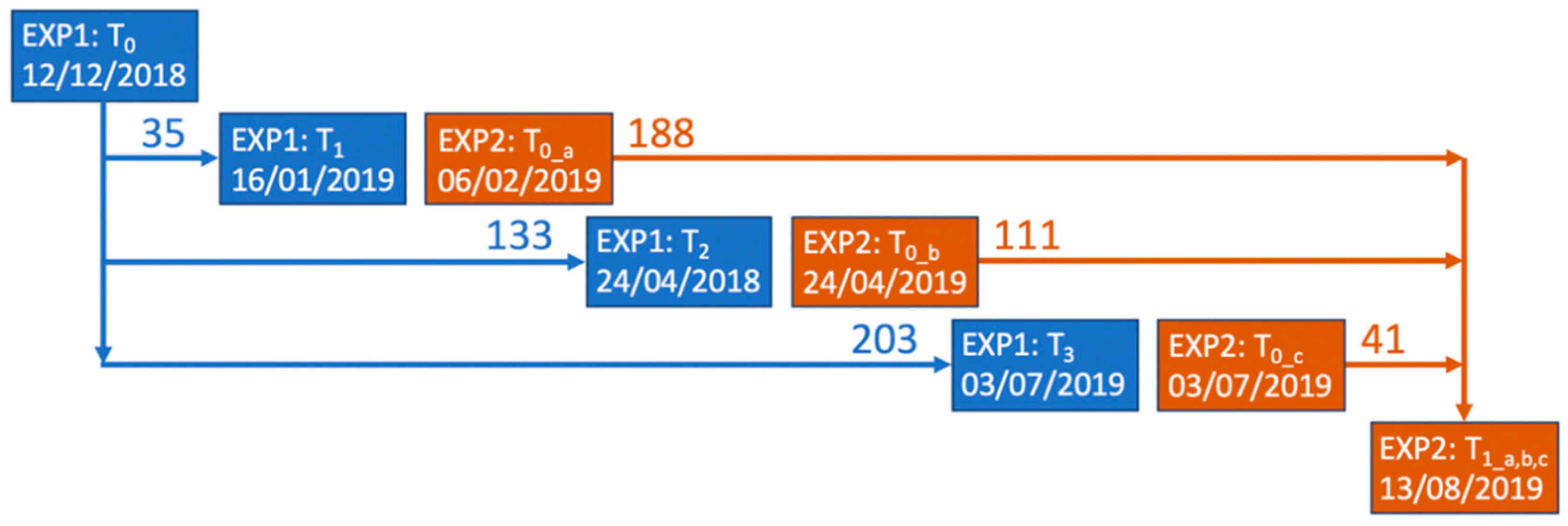
2.1. Study Site and Experimental Set-Up
2.2. Sampling Methodology
2.3. Statistical Treatment and Analysis
3. Results
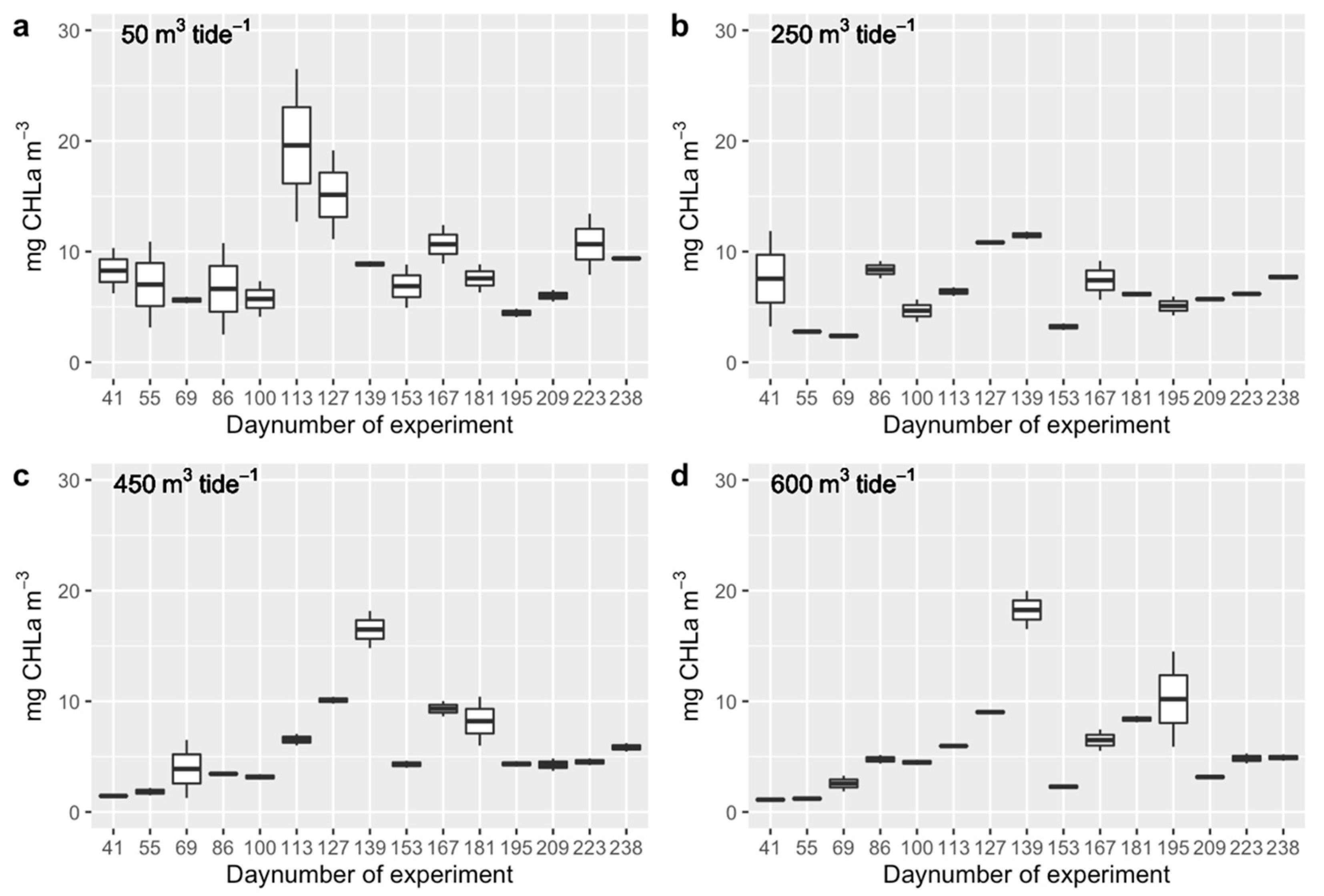
3.1. Phytoplankton
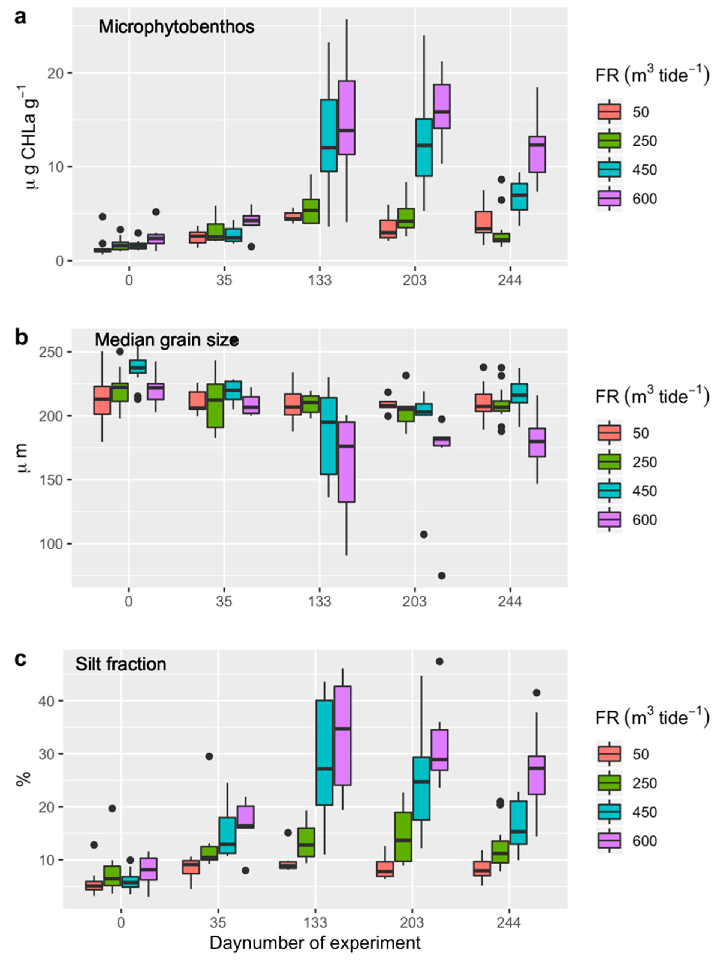
3.2. Microphytobentos
3.3. Sediment Characteristics
3.4. Cockles
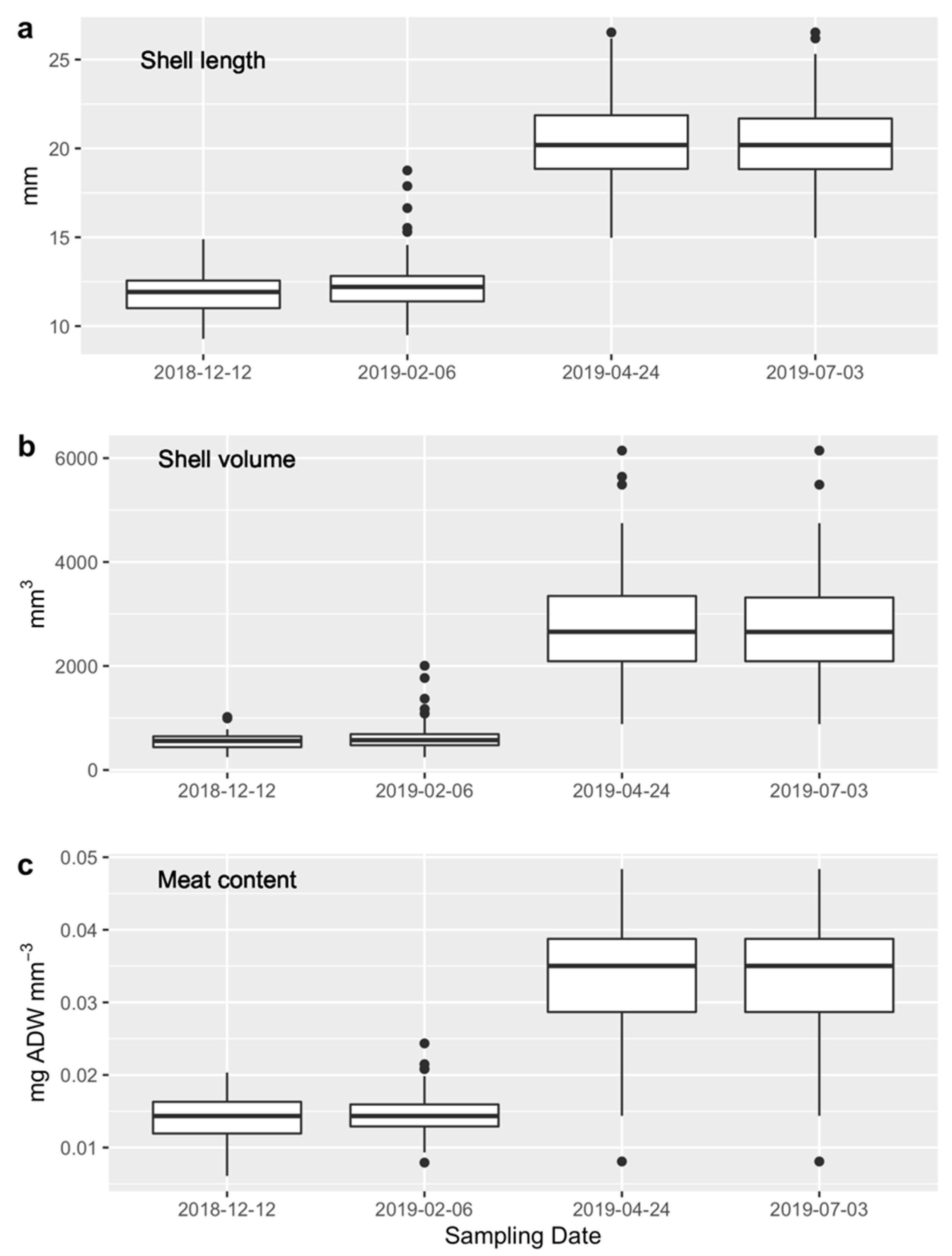
3.4.1. Juvenile Stock
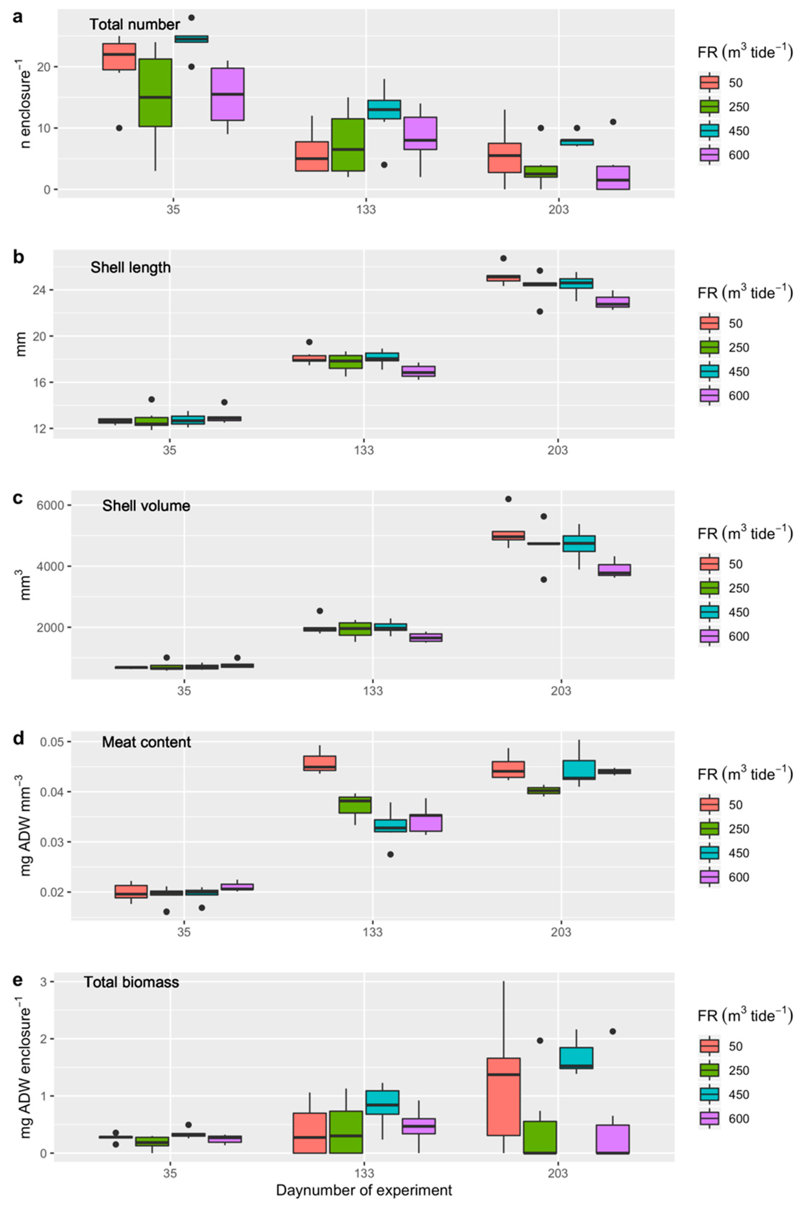
3.4.2. Experiment 1
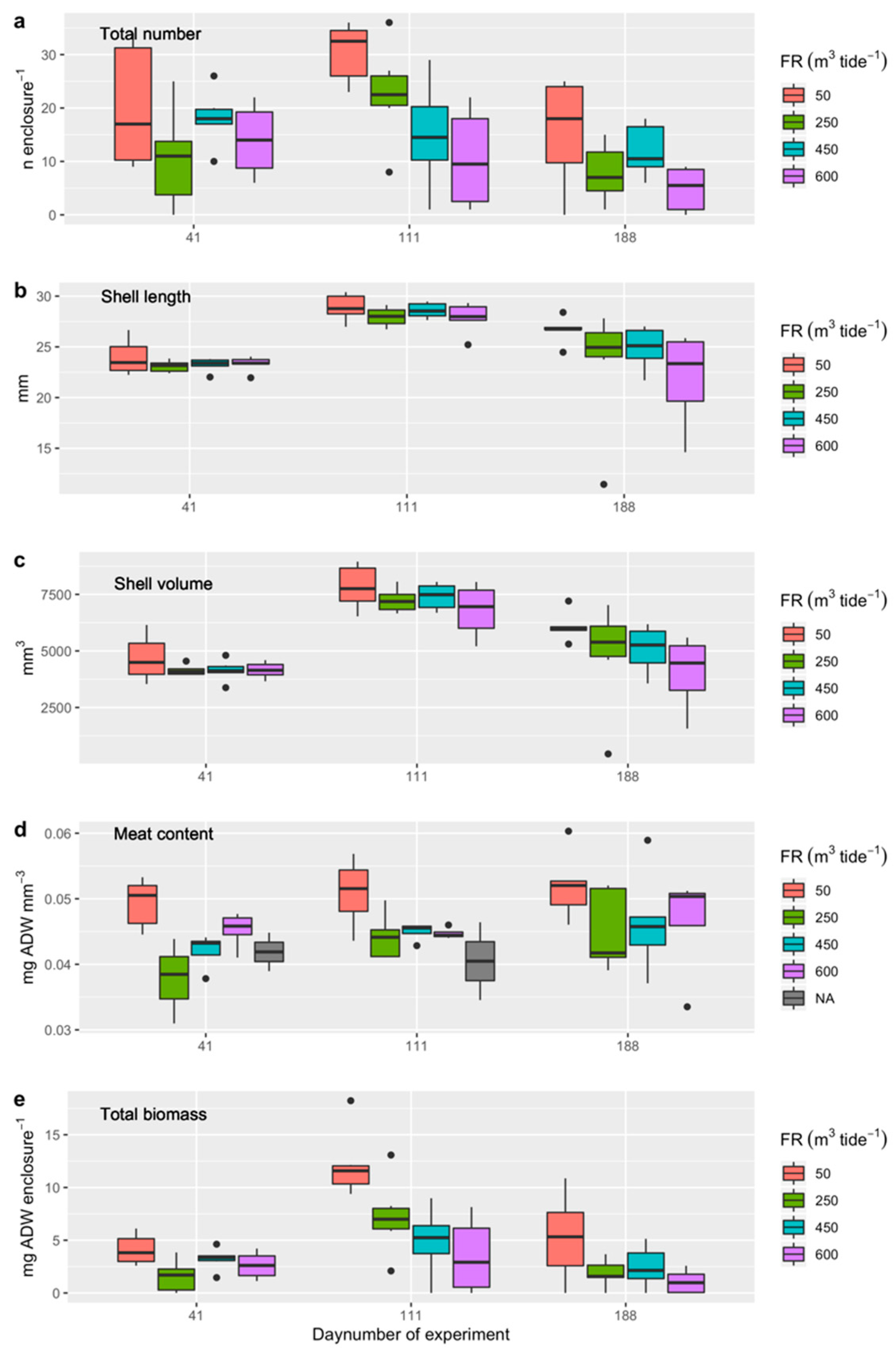
3.4.3. Experiment 2
3.5. Correlations
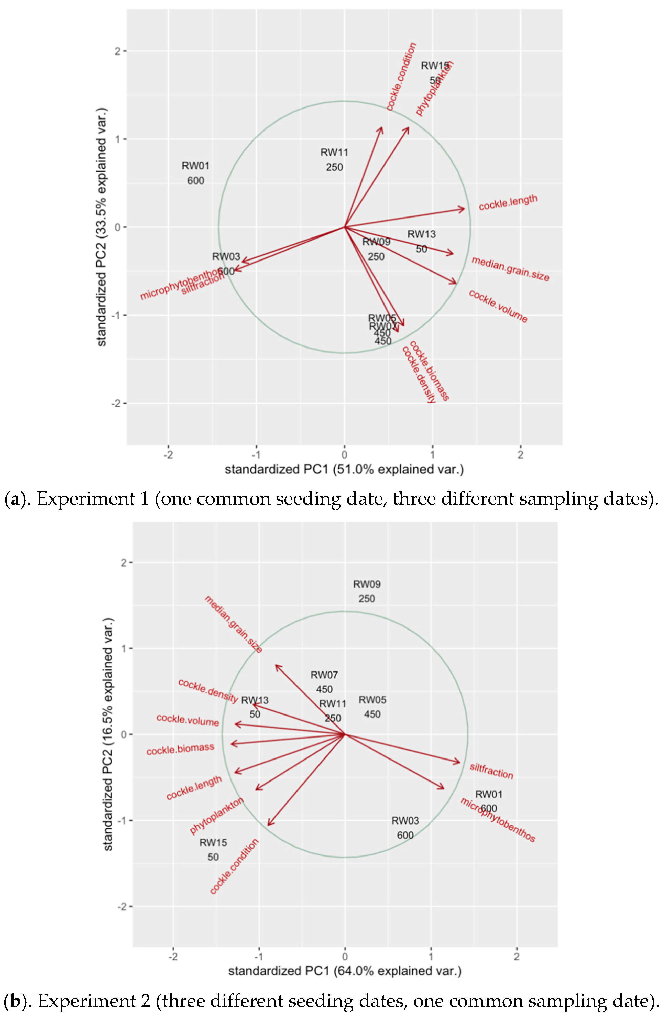
3.6. Principal Component Analyses
4. Discussion
4.1. Ecological Engineering of Environmental Conditions
4.2. Impacts on Cockle Performance Indices
4.3. Future Requirements and Perspectives
5. Conclusions
Supplementary Materials
Author Contributions
Funding
Acknowledgments
Conflicts of Interest
References
- FAO: 2018. Available online: http://www.fao.org/state-of-fisheries-aquaculture (accessed on 1 October 2020).
- Rozema, J.; Flowers, T. Crops for a salinized world. Science 2008, 322, 1478–1480. [Google Scholar] [CrossRef] [PubMed]
- Watson, R.; Cheung, W.W.L.; Anticamara, J.; Sumaila, R.U.; Zeller, D.; Pauly, D. Global marine yield halved as fishing intensity redoubles. Fish Fish. 2012, 14, 493–503. [Google Scholar] [CrossRef]
- Free, C.M.; Thorson, J.T.; Pinsky, M.L.; Oken, K.L.; Wiedenmann, J.; Jensen, O.P. Impacts of historical warming on marine fisheries production. Science 2019, 363, 979–983. [Google Scholar] [CrossRef] [PubMed]
- Waite, R.; Beveridge, M.; Brummett, R.; Chaiyawannakarn, N.; Kaushik, S.; Mungkung, R.; Nawapakpilai, S.; Phillips, M. Improving Productivity and Environmental Performance of Aquaculture; World Resource Institute: Washington, DC, USA, 2014. [Google Scholar]
- Gentry, R.R.; Ruff, E.O.; Lester, S.E. Temporal patterns of adoption of mariculture innovation globally. Nat. Sustain. 2019, 2, 949–956. [Google Scholar] [CrossRef]
- Naylor, R.L.; Williams, S.L.; Strong, D.R. Aquaculture—A Gateway for Exotic Species. Science 2001, 294, 1655–1656. [Google Scholar] [CrossRef]
- Kumar, G.; Engle, C.; Tucker, C. Factors driving aquaculture technology adoption. J. World Aquac. Soc. 2018, 49, 447–476. [Google Scholar] [CrossRef]
- Guillen, J.; Natale, F.; Carvalho, N.; Casey, J.; Hofherr, J.; Druon, J.-N.; Fiore, G.; Gibin, M.; Zanzi, A.; Martinsohn, J.T. Global seafood consumption footprint. Ambio 2019, 48, 111–122. [Google Scholar] [CrossRef]
- Oyinlola, M.A.; Reygondeau, G.; Wabnitz, C.C.; Cheung, W.L. Projecting global mariculture diversity under climate change. Glob. Chang. Biol. 2020, 26, 2134–2148. [Google Scholar] [CrossRef]
- Tyler-Walters, H. Cerastoderma edule Common cockle. In Marine Life Information Network: Biology and Sensitivity Key Information Reviews, [On-Line]; Tyler-Walters, H., Hiscock, K., Eds.; Marine Biological Association of the United Kingdom: Plymouth, UK, 2007. [Google Scholar]
- Malham, S.K.; Hutchinson, T.H.; Longshaw, M. A review of the biology of European cockles (Cerastoderma spp.). J. Mar. Biol. Assoc. UK 2012, 92, 1563–1577. [Google Scholar] [CrossRef]
- Ricardo, F.; Génio, L.; Costa Leal, M.; Albuquerque, R.; Queiroga, H.; Rosa, R.; Calado, R. Trace element fingerprinting of cockle (Cerastoderma edule) shells can reveal harvesting location in adjacent areas. Nat. Sci. Rep. 2015, 5, 11932. [Google Scholar] [CrossRef]
- Thomas Jensen, K. Density-dependent growth in cockles (Cerastoderma edule): Evidence from interannual comparisons. J. Mar. Biol. Assoc. UK 1993, 73, 333–342. [Google Scholar] [CrossRef]
- Carss, D.N.; Brito, A.C.; Chainho, P.; Ciutat, A.; de Montaudouin, X.; Fernández Otero, R.M.; Filgueira, M.I.; Garbutt, A.; Goedknegt, M.A.; Lynch, S.A.; et al. Ecosystem services provided by a non-cultured shellfish species: The common cockle Cerastoderma edule. Mar. Environ. Res. 2020, 158, 104931. [Google Scholar] [CrossRef] [PubMed]
- Hayward, P.J.; Ryland, J.S. Handbook of the Marine Fauna of North-West Europe; Oxford University Press: Oxford, UK, 1995. [Google Scholar]
- Compton, T.J.; Rijkenberg, M.J.A.; Drent, J.; Piersma, T. Thermal tolerance ranges and climate variability: A comparison between bivalves from differing climates. J. Exp. Mar. Biol. Ecol. 2007, 352, 200–211. [Google Scholar] [CrossRef]
- Modéran, J.; David, V.; Bouvais, P.; Richard, P.; Fichet, D. Organic matter exploitation in a highly turbid environment: Planktonic food web in the Charente estuary, France. Estuar. Coast. Shelf Sci. 2012, 98, 126–137. [Google Scholar] [CrossRef]
- Navarro, J.; Widdows, J. Feeding physiology of Cerastoderma edule in response to a wide range of seston concentrations. Mar. Ecol. Prog. Ser. 1997, 152, 175–186. [Google Scholar] [CrossRef]
- Christianen, M.J.A.; Middelburg, J.J.; Holthuijsen, S.J.; Jouta, J.; Compton, T.J.; van der Heide, T.; Piersma, T.; Damste, J.S.S.; van der Veer, H.W.; Schouten, S.; et al. Benthic primary producers are key to sustain the Wadden Sea food web: Stable carbon isotope analysis at landscape scale. Ecology 2017, 98, 1498–1512. [Google Scholar] [CrossRef]
- Jung, A.S.; van der Veer, H.W.; van der Meer, M.T.J.; Philippart, C.J.M. Seasonal variation in the diet of estuarine bivalves. PLoS ONE 2019, 14, e0217003. [Google Scholar] [CrossRef]
- Asmus, R.; Jensen, M.H.; Jensen, K.M.; Kristensen, E.; Asmus, H.; Wille, A. The role of water movement and spatial scaling for measurement of dissolved inorganic nitrogen fluxes in intertidal sediments. Estuar. Coast. Shelf Sci. 1998, 46, 221–232. [Google Scholar] [CrossRef]
- Ly, J.; Philippart, C.J.M.; Kromkamp, J.C. Phosphorus limitation during a phytoplankton spring bloom in the western Dutch Wadden Sea. J. Sea Res. 2014, 88, 109–140. [Google Scholar] [CrossRef]
- Stelling, G.S.; Duinmeijer, S.P.A. A staggered conservative scheme for every Froude number in rapidly varied shallow water flows. Int. J. Numer. Methods Fluids 2003, 43, 1329–1354. [Google Scholar] [CrossRef]
- Prinsen, G.F.; Becker, B.P.J. Application of SOBEK hydraulic surface water models in the Netherlands Hydrological Modelling Instrument. Irrig. Drain. 2011, 60, 35–41. [Google Scholar] [CrossRef]
- Savari, A.; Lockwood, A.P.M.; Sheader, M. Variation in the physiological state of the common cockle (Cerastoderma edule (L.)) in the laboratory and in Southampton Water. J. Molluscan Stud. 1991, 57, 33–34. [Google Scholar] [CrossRef]
- Andserson, D.R.; Burnham, K.P. Avoiding Pitfalls When Using Information-Theoretic Methods. J. Wildl. Manag. 2002, 66, 910–916. [Google Scholar]
- Bro, R.; Smilde, A.K. Principal component analysis. Anal. Methods 2014, 6, 2812–2831. [Google Scholar] [CrossRef]
- R Core Team. R: A Language and Environment for Statistical Computing; R Foundation for Statistical Computing: Vienna, Austria, 2013; Available online: http://www.R-project.org/ (accessed on 1 October 2020).
- RStudio Team. RStudio: Integrated Development for R. RStudio; PBC: Boston, MA, USA, 2020; Available online: http://www.rstudio.com/ (accessed on 1 October 2020).
- Wood, S.N. Generalized Additive Models: An Introduction with R, 2nd ed.; Chapman and Hall/CRC Press: Boca Raton, FL, USA, 2017. [Google Scholar]
- Barton, K. Package ‘MuMIn’. Model Selection and Model Averaging Based on Information Criteria. R Package Version 1.43.17. 2020. Available online: http://cran.r-project.org/web/packages/MuMIn/MuMIn.pdf (accessed on 1 October 2020).
- Loebl, M.; Colijn, F.; van Beusekom, J.E.E.; Baretta-Bekker, J.G.; Lancelot, C.; Philippart, C.J.M.; Rousseau, V.; Wiltshire, K.H. Recent patterns in potential phytoplankton limitation along the Northwest European continental coast. J. Sea Res. 2009, 61, 34–43. [Google Scholar] [CrossRef]
- Tillmann, U.; Hesse, K.-J.; Colijn, F. Planktonic primary production in the German Wadden Sea. J. Plankton Res. 2000, 22, 1253–1276. [Google Scholar] [CrossRef]
- Lumborg, U.; Pejrup, M. Modelling of cohesive sediment transport in a tidal lagoon—An annual budget. Mar. Geol. 2005, 218, 1–16. [Google Scholar] [CrossRef]
- Chang, T.S.; Bartholoma, A.; Flemming, B.W. Seasonal dynamics of fine-grained sediments in a back-barrier tidal basin of the German Wadden Sea (southern North Sea). J. Coast. Res. 2006, 22, 328–338. [Google Scholar] [CrossRef]
- Brotas, V.; Cabrita, T.; Portugal, A.; Serôdio, J.; Catarino, F. Spatio-temporal distribution of the microphytobenthic biomass in intertidal flats of Tagus Estuary (Portugal). In Space Partition within Aquatic Ecosystems; Springer: Dordrecht, The Netherlands, 1995; pp. 93–104. [Google Scholar]
- Ubertini, M.; Lefebvre, S.; Gangnery, A.; Grangeré, K.; Le Gendre, R.; Orvain, F. Spatial variability of benthic-pelagic coupling in an estuary ecosystem: Consequences for microphytobenthos resuspension phenomenon. PLoS ONE 2012, 7, e44155. [Google Scholar] [CrossRef]
- Orvain, F.; Sauriau, P.-G.; Sygut, A.; Joassard, L.; Le Hir, P. Interacting effects of Hydrobia ulvae bioturbation and microphytobenthos on the erodibility of mudflat sediments. Mar. Ecol. Prog. Ser. 2004, 278, 205–233. [Google Scholar] [CrossRef]
- Daggers, T.D.; Herman, P.M.J.; van der Wal, D. Seasonal and spatial variability in patchiness of microphytobenthos on intertidal flats from Sentinel-2 satellite imagery. Front. Mar. Sci. 2020, 7, 392. [Google Scholar]
- Foster-Smith, R.L. The effect of concentration of suspension on the filtration rates and pseudofaecal production of Mytilus edulis L.; Cerastoderma edule (L.) and Venerupis pullastra (Montagu). J. Exp. Mar. Biol. Ecol. 1975, 17, 1–22. [Google Scholar] [CrossRef]
- Beukema, J.J.; Dekker, J. Winters not too cold, summers not too warm: Long-term effects of climate change on the dynamics of a dominant species in the Wadden Sea: The cockle Cerastoderma edule L. Mar. Biol. 2020, 167, 44. [Google Scholar] [CrossRef]
- Jensen, K.T. Dynamics and growth of the cockle, Cerastoderma edule, on an intertidal mud-flat in the Danish Wadden Sea: Effects of submersion time and density. Neth. J. Sea Res. 1992, 28, 335–345. [Google Scholar] [CrossRef]
- Kamermans, P. Food limitation in cockles (Cerastoderma edule (L.)): Influences of location on tidal flat and of nearby presence of mussel beds. J. Sea Res. 1993, 31, 71–81. [Google Scholar]
- Sauriau, P.-G.; Kang, C.-K. Stable isotope evidence of benthic microalgae-based growth and secondary production in the suspension feeder Cerastoderma edule (Mollusca, Bivalvia) in the Marennes-Oléron Bay. Hydrobiologia 2000, 440, 317–329. [Google Scholar] [CrossRef]
- Prins, T.C.; Smaal, A.C.; Pouwer, A.J. Selective ingestion of phytoplankton by the bivalves Mytilus edulis l. and Cerastoderma edule (L.). Hydrobiol. Bull. 1991, 25, 93–100. [Google Scholar]
- Compton, T.J.; Holthuijsen, S.; Koolhaas, A.; Dekinga, A.; ten Horn, J.; Smith, J.; Galama, Y.; Brugge, M.; van der Wal, D.; van der Meer, J.; et al. Distinctly variable mudscapes: Distribution gradients of intertidal macrofauna across the Dutch Wadden Sea. J. Sea Res. 2013, 82, 103–116. [Google Scholar]
- Peteiro, L.G.; Woodin, S.A.; Wethey, D.S.; Costas-Costas, D.; Martínez-Casal, A.; Olabarria, C.; Vázquez, E. Responses to salinity stress in bivalves: Evidence of ontogenetic changes in energetic physiology on Cerastoderma edule. Nat. Sci. Rep. 2018, 8, 8329. [Google Scholar]
- Chen, N.; Krom, M.D.; Wu, Y.; Yu, D.; Hong, H. Storm induced estuarine turbidity maxima and controls on nutrient fluxes across river-estuary-coast continuum. Sci. Total Environ. 2018, 628, 1108–1120. [Google Scholar] [CrossRef]
- Pronker, A.E.; Peene, F.; Donner, S.; Wijnhoven, S.; Geijsen, P.; Bossier, P.; Nevejan, N.M. Hatchery cultivation of the common cockle (Cerastoderma edule L.): From conditioning to grow-out. Aquac. Res. 2015, 46, 302–312. [Google Scholar] [CrossRef]
- Kristensen, I. Differences in density and growth in a cockle population in the Dutch Wadden Sea. Arch. Neerl. Zool. 1957, 12, 351–453. [Google Scholar] [CrossRef]
- Ducrotoy, C.R.; Rybarczyk, H.; Souprayen, J.; Bachelet, G.; Beukema, J.J.; Desprez, M.; Dőrjes, J.; Essink, K.; Guillou, J.; Michaelis, H.; et al. A comparison of the population dynamics of the cockle (Cerastoderma edule) in North-Western Europe. ECSA 19. In Estuaries and Coasts: Spatial and Temporal Intercomparisons, Proceedings of the Estuarine and Coastal Sciences Association Symposium, Caen, France, 4–8 September 1989; Olsen & Olsen: Fredensborg, Denmark, 1991; pp. 173–184. [Google Scholar]
- Beukema, J.J.; Dekker, R. Decline of recruitment success in cockles and other bivalves in the Wadden Sea: Possible role of climate change, predation on postlarvae and fisheries. Mar. Ecol. Prog. Ser. 2005, 287, 149–167. [Google Scholar] [CrossRef]
- Philippart, C.J.M.; van Bleijswijk, J.D.L.; Kromkamp, J.C.; Zuur, A.F.; Herman, P.M.J. Reproductive phenology of coastal marine bivalves in a seasonal environment. J. Plankton Res. 2014, 36, 1512–1527. [Google Scholar] [CrossRef]
- André, C.; Rosenberg, R. Adult-larval interactions in the suspension-feeding bivalves Cerastoderma edule and Mya arenaria. Mar. Ecol. Prog. Ser. 1991, 71, 227–234. [Google Scholar] [CrossRef]
- Beukema, J.J.; Dekker, R. Density dependence of growth and production in a Wadden Sea population of the cockle Cerastoderma edule. Mar. Ecol. Prog. Ser. 2015, 538, 157–167. [Google Scholar] [CrossRef]
- Honkoop, P.J.C.; van der Meer, J. Experimentally induced effects of water temperature and immersion time on reproductive output of bivalves in the Wadden Sea. J. Exp. Mar. Biol. Ecol. 1998, 220, 227–246. [Google Scholar] [CrossRef]
- Langdon, C.; Evans, F.; Jacobson, D.; Blouin, M. Yields of cultured Pacific oysters Crassostrea gigas Thunberg improved after one generation of selection. Aquaculture 2003, 220, 227–244. [Google Scholar] [CrossRef]
- Avdelas, L.; Avdic-Mravlje, E.; Marques, A.C.B.; Cano, S.; Capelle, J.J.; Carvalho, N.; Cozzolino, M.; Dennis, J.; Ellis, T.; Polanco, J.M.F.; et al. The decline of mussel aquaculture in the European Union: Causes, economic impacts and opportunities. Rev. Aquac. 2020, 1–28. [Google Scholar] [CrossRef]
- Botta, R.; Asche, F.; Borsum, J.S.; Camp, E.V. A review of global oyster aquaculture production and consumption. Mar. Policy 2020, 117, 103952. [Google Scholar] [CrossRef]


| # | Hypothesis | Statistical Model | |||
|---|---|---|---|---|---|
| Factors | Smoothers | ||||
| H1 | There is one similar seasonal pattern for all raceways | M1f | yi = ßi + SamplingDatei + Ei | M1s | yi = ßi + si(SamplingDate) + Ei |
| H2 | There is one seasonal pattern, with an additional effect of raceway | M2f | yij = ßi + SamplingDatei + RaceWayj + Eij | M2s | yi = ßi + si(SamplingDate) + RaceWayj + Eij |
| H3 | There is one seasonal pattern, with an additional effect of flushing rate | M3f | yij = ßi + SamplingDatei + FlushRatek + Eik | M3s | yi = ßi + si(SamplingDate) + Flushratek + Eik |
| H4 | There is one seasonal pattern, with the additional effects of flushing rate and relative distance to inlet | M4f | yi = ßi + SamplingDatei + FlushRatek + RelDistl + Eikl | M4s | yi = ßi + si(SamplingDate) + FlushRatek + RelDistl + Eikl |
| H5 | There are different seasonal patterns per raceway | M5s | yi = ßi + sij(SamplingDate, RaceWay) + Eij | ||
| H6 | There are different seasonal patterns per flushing rate | M6s | yi = ßi + sik(SamplingDate, FlushRate) + Eik | ||
| H7 | There are different seasonal patterns per flushing rate, with an additional effect of relative distance to inlet | M7s | yi = ßi + sik(SamplingDate, FlushRate) + RelDistl + Eikl | ||
| Model | Type | Microalgal Biomass | ||
|---|---|---|---|---|
| Phytoplankton | ||||
| AIC | Δi | wi | ||
| M1 | Factors | 643.7 | 62.3 | 0.00 |
| Smoothers | 649.1 | 67.7 | 0.00 | |
| M2 | Factors | 623.4 | 42.0 | 0.00 |
| Smoothers | 633.7 | 52.3 | 0.00 | |
| M3 | Factors | 628.9 | 47.5 | 0.00 |
| Smoothers | 637.1 | 55.7 | 0.00 | |
| M4 | Factors | 627.6 | 46.2 | 0.00 |
| Smoothers | 636.3 | 54.9 | 0.00 | |
| M5 | Smoothers | 581.4 | 0.0 | 1.00 |
| M6 | Smoothers | 658.9 | 77.4 | 0.00 |
| M7 | Smoothers | 658.109 | 76.7 | 0.00 |
| Model | Sediment Characteristics | Microalgal Biomass | |||||||
|---|---|---|---|---|---|---|---|---|---|
| Median Grain Size | Silt Fraction | Microphytobenthos | |||||||
| Factors | Factors | Factors | |||||||
| AIC | Δi | wi | AIC | Δi | wi | AIC | Δi | wi | |
| M1 | 1962.8 | 35.3 | 0.00 | 1520.6 | 101.2 | 0.00 | 1220.5 | 89.8 | 0.00 |
| M2 | 1931.8 | 4.3 | 0.05 | 1424.2 | 4.8 | 0.04 | 1135.1 | 4.5 | 0.04 |
| M3 | 1927.5 | 0.0 | 0.71 | 1421.6 | 2.2 | 0.26 | 1130.7 | 0.0 | 0.65 |
| M4 | 1928.5 | 1.0 | 0.24 | 1419.4 | 0.0 | 0.70 | 1132.0 | 1.3 | 0.31 |
| Index | Model | Experiment 1 | Experiment 2 | ||||
|---|---|---|---|---|---|---|---|
| AIC | Δi | wi | AIC | Δi | wi | ||
| Density | M1 | 449.4 | 15.3 | 0.00 | 530.0 | 54.9 | 0.00 |
| M2 | 434.1 | 0.0 | 0.39 | 503.7 | 28.6 | 0.00 | |
| M3 | 436.4 | 2.3 | 0.47 | 475.1 | 0.0 | 0.79 | |
| M4 | 438.4 | 4.2 | 0.14 | 477.1 | 2.0 | 0.22 | |
| Shell length | M1 | 177.7 | 3.1 | 0.24 | 322.5 | 60.8 | 0.00 |
| M2 | 182.2 | 7.5 | 0.00 | 325.7 | 64.0 | 0.00 | |
| M3 | 174.7 | 0.0 | 0.59 | 262.5 | 0.9 | 0.47 | |
| M4 | 176.6 | 2.0 | 0.17 | 261.7 | 0.0 | 0.53 | |
| Shell volume | M1 | 1228.6 | 2.5 | 0.28 | 1266.5 | 108.6 | 0.00 |
| M2 | 1231.8 | 5.7 | 0.01 | 1267.6 | 109.7 | 0.00 | |
| M3 | 1226.1 | 0.0 | 0.54 | 1157.9 | 0.0 | 0.63 | |
| M4 | 1227.9 | 1.8 | 0.17 | 1158.3 | 0.5 | 0.37 | |
| Meat content | M1 | −199.6 | 3.5 | 0.22 | −174.1 | 43.9 | 0.00 |
| M2 | −202.8 | 0.3 | 0.07 | −218.0 | 0.0 | 1.00 | |
| M3 | −203.1 | 0.0 | 0.56 | −179.9 | 38.1 | 0.00 | |
| M4 | −201.2 | 2.0 | 0.15 | −193.1 | 24.9 | 0.00 | |
| Total biomass | M1 | 467.0 | 9.3 | 0.02 | 708.4 | 78.0 | 0.00 |
| M2 | 457.7 | 0.0 | 0.31 | 687.7 | 57.3 | 0.00 | |
| M3 | 460.2 | 2.5 | 0.34 | 630.4 | 0.0 | 0.65 | |
| M4 | 459.8 | 2.1 | 0.32 | 631.0 | 0.7 | 0.35 | |
| Group | Variable 1 | Variable 2 | Experiment 1 | Experiment 2 | ||
|---|---|---|---|---|---|---|
| R | p | R | p | |||
| Environmental conditions | Phytoplankton | Microphytobenthos | −0.479 | 0.229 | Similar to Experiment 1 | |
| Median grain size | 0.239 | 0.569 | ||||
| Silt fraction | −0.643 | 0.085 | ||||
| Microphyto-benthos | Median grain size | −0.604 | 0.113 | |||
| Silt fraction | 0.960 | 0.000 | ||||
| Median grain size | Silt fraction | −0.600 | 0.116 | |||
| Cockle performance indices | Density | Shell length | 0.312 | 0.452 | 0.544 | 0.164 |
| Shell volume | 0.714 | 0.047 | 0.675 | 0.066 | ||
| Condition | −0.397 | 0.330 | 0.268 | 0.520 | ||
| Total biomass | 0.945 | 0.000 | 0.878 | 0.004 | ||
| Shell length | Shell volume | 0.743 | 0.035 | 0.877 | 0.004 | |
| Meat content | 0.481 | 0.228 | 0.813 | 0.014 | ||
| Total biomass | 0.382 | 0.350 | 0.791 | 0.019 | ||
| Shell volume | Condition | −0.132 | 0.755 | 0.521 | 0.186 | |
| Total biomass | 0.747 | 0.033 | 0.760 | 0.029 | ||
| Meat content | Total biomass | −0.278 | 0.505 | 0.596 | 0.119 | |
| Cross correlations | Cockle density | Phytoplankton | −0.327 | 0.429 | 0.233 | 0.579 |
| Microphytobenthos | 0.014 | 0.973 | −0.641 | 0.087 | ||
| Median grain size | 0.474 | 0.236 | 0.288 | 0.489 | ||
| Silt fraction | −0.046 | 0.913 | −0.691 | 0.058 | ||
| Cockle length | Phytoplankton | 0.633 | 0.092 | 0.730 | 0.040 | |
| Microphytobenthos | −0.714 | 0.047 | −0.493 | 0.215 | ||
| Median grain size | 0.810 | 0.015 | 0.457 | 0.255 | ||
| Silt fraction | −0.804 | 0.016 | −0.696 | 0.055 | ||
| Cockle volume | Phytoplankton | 0.062 | 0.883 | 0.495 | 0.212 | |
| Microphytobenthos | −0.646 | 0.084 | −0.620 | 0.101 | ||
| Median grain size | 0.843 | 0.009 | 0.658 | 0.076 | ||
| Silt fraction | −0.648 | 0.082 | −0.760 | 0.029 | ||
| Cockle meat content | Phytoplankton | 0.931 | 0.001 | 0.719 | 0.045 | |
| Microphytobenthos | −0.207 | 0.622 | −0.172 | 0.685 | ||
| Median grain size | 0.039 | 0.928 | −0.023 | 0.957 | ||
| Silt fraction | −0.392 | 0.337 | −0.418 | 0.303 | ||
| Cockle biomass | Phytoplankton | −0.277 | 0.506 | 0.663 | 0.073 | |
| Microphytobenthos | −0.016 | 0.969 | −0.710 | 0.049 | ||
| Median grain size | 0.471 | 0.238 | 0.293 | 0.481 | ||
| Silt fraction | −0.071 | 0.868 | −0.834 | 0.010 | ||
© 2020 by the authors. Licensee MDPI, Basel, Switzerland. This article is an open access article distributed under the terms and conditions of the Creative Commons Attribution (CC BY) license (http://creativecommons.org/licenses/by/4.0/).
Share and Cite
Philippart, C.J.M.; Dethmers, K.E.M.; van der Molen, J.; Seinen, A. Ecological Engineering for the Optimisation of the Land-Based Marine Aquaculture of Coastal Shellfish. Int. J. Environ. Res. Public Health 2020, 17, 7224. https://doi.org/10.3390/ijerph17197224
Philippart CJM, Dethmers KEM, van der Molen J, Seinen A. Ecological Engineering for the Optimisation of the Land-Based Marine Aquaculture of Coastal Shellfish. International Journal of Environmental Research and Public Health. 2020; 17(19):7224. https://doi.org/10.3390/ijerph17197224
Chicago/Turabian StylePhilippart, Catharina J. M., Kiki E. M. Dethmers, Johan van der Molen, and André Seinen. 2020. "Ecological Engineering for the Optimisation of the Land-Based Marine Aquaculture of Coastal Shellfish" International Journal of Environmental Research and Public Health 17, no. 19: 7224. https://doi.org/10.3390/ijerph17197224
APA StylePhilippart, C. J. M., Dethmers, K. E. M., van der Molen, J., & Seinen, A. (2020). Ecological Engineering for the Optimisation of the Land-Based Marine Aquaculture of Coastal Shellfish. International Journal of Environmental Research and Public Health, 17(19), 7224. https://doi.org/10.3390/ijerph17197224