Abstract
High air pollution levels have become a nationwide problem in China, but limited attention has been paid to prefecture-level cities. Furthermore, different time resolutions between air pollutant level data and meteorological parameters used in many previous studies can lead to biased results. Supported by synchronous measurements of air pollutants and meteorological parameters, including PM2.5, PM10, total suspended particles (TSP), CO, NO2, O3, SO2, temperature, relative humidity, wind speed and direction, at 16 urban sites in Xiangyang, China, from 1 March 2018 to 28 February 2019, this paper: (1) analyzes the overall air quality using an air quality index (AQI); (2) captures spatial dynamics of air pollutants with pollution point source data; (3) characterizes pollution variations at seasonal, day-of-week and diurnal timescales; (4) detects weekend effects and holiday (Chinese New Year and National Day holidays) effects from a statistical point of view; (5) establishes relationships between air pollutants and meteorological parameters. The principal results are as follows: (1) PM2.5 and PM10 act as primary pollutants all year round and O3 loses its primary pollutant position after November; (2) automobile manufacture contributes to more particulate pollutants while chemical plants produce more gaseous pollutants. TSP concentration is related to on-going construction and road sprinkler operations help alleviate it; (3) an unclear weekend effect for all air pollutants is confirmed; (4) celebration activities for the Chinese New Year bring distinctly increased concentrations of SO2 and thereby enhance secondary particulate pollutants; (5) relative humidity and wind speed, respectively, have strong negative correlations with coarse particles and fine particles. Temperature positively correlates with O3.
1. Introduction
Air pollution is caused by manifold particulate and gaseous pollutants, namely, particles with aerodynamic diameter less than 2.5 μm (PM2.5) and less than 10 μm (PM10), and total suspended particles (TSP), carbon monoxide (CO), nitrogen dioxide (NO2), ozone (O3) and sulfur dioxide (SO2) [1]. Prolonged high levels of air pollution have been verified to have significant adverse impacts on human health: (1) particulate matters, especially fine particles, can increase the risk of cerebrovascular diseases, heart diseases, chronic obstructive pulmonary diseases (COPD), acute respiratory infections and lung cancer [2,3,4,5]; (2) intensive exposures to O3 and NO2 can lead to COPD, respiratory morbidity and premature death [2,5,6,7]; (3) high levels of CO and SO2 can cause cataracts, respiratory symptoms and COPD [2,8,9]. According to the World Health Statistics 2018 released by the World Health Organization, 7 million people are killed annually by air pollution-related diseases all over the world, and in China the number is around 1.83 million [3]. Substantial efforts to clarify air pollution distributions, and thereby to alleviate haze problems desperately need to be made.
A ground monitoring network was established by the Ministry of Ecology and Environment of China (MEEC) on 2000, and then was expanded to monitor 338 cities, with measurements of PM2.5, PM10, CO, NO2, O3 and SO2, on 2015 [10,11]. Subsequently, remarkable progress has been achieved on spatiotemporal variations of air pollutants at urban scale. Spatially, previous studies primarily focused on a specific city or comparisons between cities. Due to unevenly distributed ground monitoring stations, most investigations were carried out in key cities or environment protection mode cities [12,13,14], albeit with limited studies on fine particulate matters and air quality index (AQI) in prefecture-level cities [15,16]. Equivalent findings in temporal variabilities of air pollutants have shown interannual, seasonal, day-of-week, diurnal and specific timescale variability characteristics (i.e., haze episodes and national holidays) [15,16,17,18,19,20,21,22,23]. Nevertheless, TSP has not popularly been studied since 2001 when TSP was excluded from the China Environment Bulletin [23]. A distinct seasonal pattern for “worse winter and better summer” and traffic-related diurnal characteristics were captured by an array of studies [15,16,17,18,19,20,21,22]. Although day-of-week variations in different cities follow different rules, mean concentrations of air pollutants during weekdays are usually greater than those during weekends. However, seldom studies confirmed the weekday-weekend difference of pollution concentrations from a statistical point of view. In terms of discovering variations of pollutant concentrations during national holidays, such as the Chinese New Year (CNY), some studies have revealed a clear holiday effect which is defined as differences of air pollution concentrations during national holidays and non-holiday periods by using the independent samples -test and paired samples -test [24]. However, the non-CNY period, covering 10 days before and 10 days after CNY, is not applicable to mainland China, because a compact but prodigious population mobility that can be observed during that period, suggesting more traffic-related emissions than usual, which in turn can disrupt the holiday effect test results.
Regarding the meteorological influences, some valuable results were unveiled thanks to the open data collected by the China Meteorological Administration (CMA). Specifically, certain synoptic conditions, such as low wind speed (WS) and stagnant weather, can increase the risk of haze occurrence while strong windy and rainy weathers reasonably disrupt accumulation as well as scavenge of particles [18,19,21,23]. Meanwhile, temperature, sunshine duration and planetary boundary layer height (PBLH) are generally believed to accelerate the local photochemical formation, and thereby bring heavy secondary generated O3 pollution [18,19,21,23]. However, the publicly accessible measurements for meteorological parameters (i.e., pressure, temperature, relative humidity, precipitation, evaporation, wind speed and direction, sunshine duration, and ground surface temperature) from the CMA, on a daily time scale, are insufficient to synchronously detect meteorological effects due to the hourly variations of air pollutants. The problem of different time resolutions has been noted by some scholars [18,25]. Furthermore, air pollutants and meteorological parameters for the same city are normally measured by different stations situated at different locations, which probably generates biased results for the meteorological influences on air pollution distributions.
Supported by synchronous ground measurements of air pollutants and meteorological parameters (i.e., PM2.5, PM10, TSP, CO, NO2, O3, SO2, temperature, relative humidity, wind speed and direction), at 16 urban sites in Xiangyang from 1 March 2018 to 28 February 2019, we first analyzed the overall air quality with AQI and then captured the spatial dynamics of air pollutants with ten-kind point pollution source data. Thirdly, we characterized pollution variations on a seasonal, day-of-week and diurnal time scale, including the diagnoses of weekend effects and holiday effects by the Kruskal-Wallis rank-sum test. Finally, the Spearman’s rank correlation coefficient was strictly applied to establish relationships between air pollutants and meteorological parameters.
2. Materials and Methods
2.1. Study Area and Measurement Stations
Xiangyang is a prefecture-level city lying on the middle reaches of the Han River in central China (Figure 1), and features a subtropical monsoon climate all the year round. According to the Xiangyang Statistical Yearbook 2018, half of the Gross Domestic Product (GDP) of Xiangyang is derived from industrial production, especially from automobile manufacturers and chemical industries [26]. Consequently, severe haze episodes have been observed more frequently here. To clarify the agglomeration and diffusion mechanism of air pollution, an hourly monitoring network of air pollutants and meteorological parameters was established in the built environment of Xiangyang by the Xiangyang Environmental Monitoring Center in February 2018.
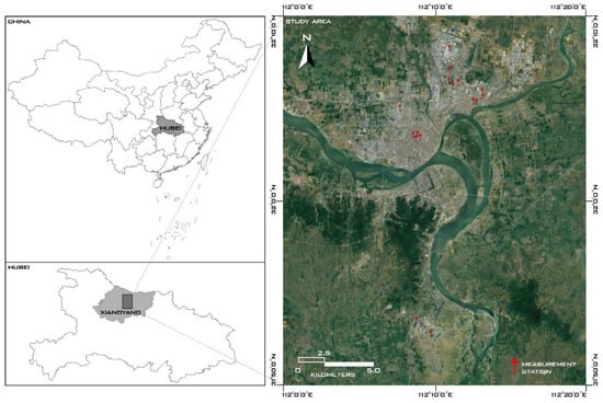
Figure 1.
The locations of the study area and 16 measurement stations.
The hourly monitoring system includes 16 measurement stations which automatically record data of seven air pollutants and four meteorological parameters, namely, particles with aerodynamic diameter less than 2.5 μm (PM2.5) and less than 10 μm (PM10), total suspended particles (TSP), carbon monoxide (CO), nitrogen dioxide (NO2), ozone (O3), sulfur dioxide (SO2), temperature, relative humidity (RH), wind speed (WS) and wind direction (WD). Based on the Chinese Ambient Air Quality Standard (GB3095-2012) and the Specifications for Surface Meteorological Observation (GB/T 35226-2017 and GB/T 35227-2017), the sampling methods are as follows: (1) tapered element oscillating microbalances together with the β-ray method are adopted to measure the mass concentrations of PM2.5, PM10 and TSP; (2) the non-dispersion infrared absorption method together with the gas filter correlation infrared method is utilized to measure the mass concentration of CO; (3) the differential optical absorption spectroscopy (DOAS) method together with the chemiluminescence method is employed to measure the mass concentration of NO2; (4) the DOAS method together with the ultraviolet fluorescence method is used to measure the mass concentrations of O3 and SO2; (5) AQMS2000 monitors (the Fairsense Ltd., Beijing, China) are installed to observe temperature, RH, WS and WD [27,28,29]. Installation and acceptance of measurement stations rely on the technical guidelines of GB/T 35226-2017, GB/T 35227-2017, HJ655-2013 and HJ193-2013 [28,29,30,31].
2.2. Data Sources
2.2.1. Data of Air Pollutants and Meteorological Parameters
In this study, we adopted continuous twelve-month data of seven air pollutants and four meteorological parameters collected by the 16 aforementioned measurement stations from 1 March 2018 to 28 February 2019. To maintain data validity in the subsequent analyses, a data check in compliance with the Chinese Ambient Air Quality Standard [27] was conducted on the platform of R, and we found some missing values for TSP, WS and WD of Station 15 and Station 16, further demonstrated to be the storage loss. Statistical summaries of hourly measurements for four meteorological parameters and seven air pollutants during the studied period were respectively listed in Table 1 and Table 2.

Table 1.
Measurement site description and statistical summaries of hourly measurements for meteorological parameters in Xiangyang from 1 March 2018 to 28 February 2019.
Table 2.
Statistical summaries of hourly measurements for air pollutants in Xiangyang from 1 March 2018 to 28 February 2019.
Notably, the data of daily urban wind speed from 1 March 2018 to 28 February 2019 downloaded from the website of CMA [32] was used to make a comparison with the WS measured by those 16 measurement stations. In addition, Station 15 and Station 16 were excluded from the subsequent analyses related to TSP variations as well as correlations between air pollutants and meteorological parameters.
As a non-dimensional index, the AQI is broadly utilized to reveal levels of air pollution and risks to human health [33,34]. In this study, the category and the calculation of AQI are based on technical specifications described by the MEEC in the HJ633-2012 (Table 3) [35]. Generally, the higher the AQI number, the worse the air condition. Equations for AQI are as follows:
where represents the individual air quality index for pollutant ; is the mass concentration for pollutant ; and respectively denote the closest upper and lower breakpoint of ; and respectively represent the corresponding to and . Detailed technical specifications of thresholds for each pollutant can be found in the HJ633-2012 [35]. Equation (2) illustrates the overall AQI number determined by the maximum of 6 including for PM2.5, PM10, TSP, CO, NO2, O3 and SO2. Meanwhile, the individual pollutant with the maximal value is defined as the primary pollutant of that day when the daily AQI number is above 50. Finally, we put the mass concentration for each pollutant in Equations (1) and (2) to obtain the daily AQI and the primary pollutant from 1 March 2018 to 28 February 2019.
Table 3.
The air quality index (AQI) and corresponding health effects.
2.2.2. Pollution Point-Source Data
Stationary pollution sources are acknowledged to have certain impacts on the spatiotemporal distribution of air pollutants. Therefore, 10 kinds of point source data, including feed mills, automobile manufacturers, automobile repair workshops, machinery manufacturers, chemical plants, electronic companies, material companies, building material companies, other industrial companies, and on-going construction sites were used to depict the surrounding built environment of each measurement station.
Locations of the industrial facilities were obtained from the Xiangyang Natural Resources and Planning Bureau (XNRPB) [36] and Google Maps (the Google LLC, Mountain View, CA, US). The list of on-going construction sites was collected from the website of Xiangyang Housing and Urban-Rural Development Bureau [37]. Then, we pinpointed them on the Google Map. Moreover, 16 buffer zones of measurement stations were created, and the optimal radius of the buffer zone was demonstrated to be 1 km by prior studies [38,39].
2.3. Methods
Strong winds or rainfalls can have scavenging effects on atmospheric pollutants, so days with daily WS over 3.4 m/s or daily precipitations over 5 mm were excluded from the subsequent analyses [40]. In addition, holidays can also disrupt the results. Specifically, most work plants do not produce on weekends, and if a Saturday or a Sunday happens to be a working day, the final mean concentration of air pollutants on Saturday or Sunday will probably be higher than the true value. Thus, if a day from Monday to Friday happens to be a holiday or if a Saturday or a Sunday happens to be a working day, we excluded that day from the analyses for the day-of-week variations. Other notable details in this study were listed here: (1) particulate pollutants encompass PM2.5, PM10 as well as TSP, and air pollutants stand for particulate pollutants along with gaseous pollutants; (2) the data of WS, temperature and RH participating in the Spearman’s rank test were collected by the 16 measurement stations.
Daily mean concentrations were averaged by hourly measurements, and monthly mean concentrations were respectively averaged by daily and monthly mean concentrations. Analogously, we obtained the mean concentrations of air pollutants for diurnal analysis. Spatially, the annual mean concentrations of air pollutants for each measurement station were averaged by using the corresponding daily mean concentrations. CNY and National Day (NDH) holidays are the equally longest holidays (7 days) in mainland China, and significant behavioral changes from usual days can be observed during CNY and NDH. Specifically, CNY is the most important holiday for Chinese people to get together, resulting in a compact but prodigious population mobilization from a week before to a week after CNY. Meanwhile, many work plants and construction sites are closed for several days during CNY and NDH. Moreover, celebration activities (i.e., setting off firecrackers, burning paper money to worship ancestors on New Year’s Eve, etc.), temporarily permitted by the government, can also be observed during the CNY. To sum it up, with reduced local stationary emissions, CNY and NDH are suitable study periods to conduct a diagnosis of the holiday effect [24,41]. To rule out meteorological influences, we defined the non-holiday period for CNY (non-CNY period) as the time interval from 1 December 2018 to 28 February 2019 excluding CNY and the non-holiday period for NDH (non-NDH period) as the time interval from 1 September 2018 to 30 November 2018 excluding NDH. Then, we discovered that not all data of air pollutants comply with the normal distribution by carrying out the Kolmogorov-Smirnov test. Given the fact that the Kruskal-Wallis rank-sum test is a widely used nonparametric approach to examine differences between multi-independent group samples with unknown distributions [16], it was introduced in our study after a Chi-square test confirming the seven air pollutants are independent from each other. Subsequently, we conducted the Kruskal-Wallis test at the significant level of 5% and the null hypothesis () is no significant differences of distributions of air pollutants during holidays and non-holiday period. When the value of this test is less than 0.05, the will be rejected, suggesting an obvious holiday effect, and vice versa. We repeated the same approach to examine the weekday-weekend statistical difference of air pollution concentrations. Finally, the Spearman’s rank correlation coefficient was introduced to identify relationships between air pollutants and meteorological parameters. Notably, the Kruskal-Wallis test was realized on the platform of R and the Kolmogorov-Smirnov test as well as the Spearman’s rank test was processed on the MATLAB R2015b (the MathWorks Inc., Natick, MA, US).
3. Results and Discussion
3.1. Overview of Air Quality
The annual AQI average in Xiangyang on all measurements from 1 March 2018 to 28 February 2019 is 102.0 ± 51.2. The monthly AQI average exhibited a cosinoidal pattern, as shown in Figure 2. The air quality keeps ameliorating after March, and then maintains a steadily good condition from July to October. Nevertheless, the air quality deteriorates after October, and reached the worst condition in January, 2019. Regarding the percentage of the days with different air quality, the result was ranked in a decreasing order: excellent and good air quality day (64.6%) > slightly polluted day (21.5%) > moderately polluted day (7.9%) > heavily polluted day (6.0%) > severely polluted day (0). The percentage of days with excellent and good air quality fails in reaching the criteria of 80% proposed by China’s 13th Five-Year Plan (2016–2020). Furthermore, in order to better understand the contribution of air pollutants to the AQI, the primary pollutants over the same time interval were calculated by months (Figure 2). The year-round air quality in Xiangyang mainly deteriorates due to the joint effect of three primary pollutants, namely, PM2.5, O3 and PM10, accounting for 52.1%, 27.4% and 14.2% respectively. PM2.5 and PM10 act as the primary pollutant all the year round, by contrast, O3 loses its position of primary pollutant since November. The main reason for O3 to be considered as the dominant primary pollutant in summer is that high temperature, along with more hours of sunlight, helps accelerate the local photochemical formation [11,14,42]. The contingently one-time occurrence of NO2 as the primary pollutant might be the result of a long-range transported pollution from neighboring regions. Compared with prior studies in Beijing, SO2 is not one of primary pollutants even in winter. The variability is probably derived from coal-fired heating extensively used during winter in the north of China [1].
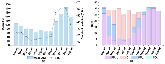
Figure 2.
Characteristics of the air quality index (AQI) and the primary pollutants to AQI in Xiangyang by months from March 1, 2018 to February 28, 2019: (a) AQI; (b) primary pollutants.
3.2. Spatial Variations of Particulate and Gaseous Pollutants
The locations of 16 measurement stations and their annual concentrations of air pollutants are displayed in Figure 3 and Table 4. Obviously, annual concentrations of PM2.5 and PM10 measured by all stations strikingly exceed both the Chinese National Ambient Air Quality Standards (CNAAQS) [27] and the World Health Organization Air Quality Guidelines (WHOAQG) [43]. Spatially, the largest annual values of gaseous pollutants are identically reported by Station 15 while the maximal annual concentrations of particulate pollutants are from Station 6. The highest level of each gaseous pollutant of Station 15 is caused by nine nearby chemical plants. However, Station 16, also surrounded by nine chemical plants, has relatively less concentrations of gaseous pollutants when compared to Station 15. By field investigation, we figured out that the difference is mainly ascribed to the location of the monitor. The monitor of Station 15 is inside a fertilizer factory, whereas the monitor of Station 16 is 10 m away from the factory gate.
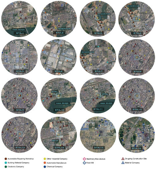
Figure 3.
Pollution sources within one-kilometer-radius buffer zones of 16 measurement stations.
Table 4.
Annual mean concentrations of 16 measurement stations in Xiangyang from 1 March 2018 to 28 February 2019.
The most abundant concentrations of particulate pollutants of Station 6 are closely associated with the land use made by automobile manufacture, accounting for four automobile work plants, three machinery factories and two electronics factories. It also suggests that automotive plants contribute to more particulate pollutants rather than gaseous pollutants while chemical plants emit more gaseous pollution. Meanwhile, Station 2 recorded the minimal annual concentrations of particulate pollutants and SO2 due to its location in a residential area. In addition, interesting results of heterogeneous variations for air pollutants between some adjacent stations were uncovered. Specifically, Station 3 and Station 7 (distance of 500 m) as well as Station 14 and Station 1 (distance of 565 m) show relatively uniform annual variations of gaseous pollutants while vary from annual concentrations of particulate pollutants (especially TSP). Different numbers of on-going construction sites are responsible for the variability. Specifically, Station 3 and Station 14 with more on-going construction sites inevitably produce more resuspended dust. It also can be seen that Station 10 and Station 11 (distance of 377 m) have the same number of on-going construction sites, but Station 11 monitors larger TSP concentrations, as Station 11 closer to construction sites. Station 9, Station 8, Station 11 and Station 13 also have several on-going construction sites in the buffer zone, but their annual concentrations of TSP are relatively lower. With reference to the urban management information on the website of XNRPB [36], one possible reason is that road sprinkler operations help deposit TSP.
3.3. Temporal Variations of Particulate and Gaseous Pollutants
3.3.1. Seasonal Characteristics
Seasonal averages of PM2.5, PM10, TSP, NO2 and SO2 similarly exhibit U-shaped patterns with the common feature of the maximum being in winter while the minimum being in summer. Conversely, the seasonal mean concentration of O3 interestingly presents an inverted U-shaped pattern (Figure 4). The reason for the phenomenon is that lower temperature and less hours of sunlight in winter are unfavorable to photochemical activities, and then interfere with the O3 formation. Meanwhile, lower PBLH along with stagnant synoptic conditions in winter has adverse effects on particles diffusion [1,14,44]. The seasonal average of O3 slightly increases from spring to summer, and then strikingly decreases from summer to winter. This echoes the fact that O3 loses its position of primary pollutant since November as previously discovered. By contrast, the seasonal mean concentration of CO maintains a relatively stable level and a slight peak appears in winter.
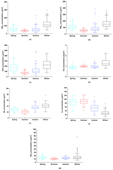
Figure 4.
Seasonal variations of air pollutants in Xiangyang from March 1, 2018 to February 28, 2019: (a) PM2.5; (b) PM10; (c) total suspended particles (TSP); (d) CO; (e) NO2; (f) O3; (g) SO2.
3.3.2. Concentration Changes during Chinese New Year and National Day Holidays
The results of the difference tests of NDH-nonNDH and CNY-nonCNY on all measurements were listed in Table 5. Significant differences of concentrations of NO2 and SO2 during NDH and non-NDH were uncovered. Specifically, the mean concentrations of NO2 and SO2 during NDH are higher than those during non-NDH, despite many plants being off-line during NDH. To further illustrate the results, we visualized the daily and weekly variations from a week before NDH to a week after NDH (24 September 2018 to 14 October 2018) in Figure 5. Generally, during NDH, the mean concentrations of PM2.5, PM10, TSP, NO2 and O3 respectively show a similarly dramatic uptrend and the mean concentration of CO exhibits a slight increase. However, the mean concentration of SO2 interestingly maintains a stable level. Notably, concentrations of all air pollutants reach the peak during the period from October 7 to October 9. After having checked the wind direction and air pollution information of neighboring provinces, we discovered that the higher concentrations during NDH can probably be ascribed to the pollution transported by the northeast wind from Henan Province.
Table 5.
Results of holiday-nonholiday difference tests at 16 measurement stations.
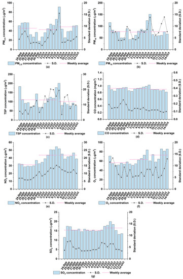
Figure 5.
Daily variations of mean concentrations for air pollutants in Xiangyang from a week before National Day holidays to a week after National Day holidays: (a) PM2.5; (b) PM10; (c) TSP; (d) CO; (e) NO2; (f) O3; (g) SO2.
Significant differences of the NO2 concentration and the O3 concentration during CNY and non-CNY were unveiled, and the mean concentration of NO2 during non-CNY is much greater than that during CNY. The result is primarily ascribed to suspended industrial productions, engineering constructions, etc. during CNY, suggesting reduced stationary emissions over that time interval. It also can be seen from Figure 6 that trends of mean concentrations for PM2.5, PM10, TSP, CO and SO2 during CNY fluctuate like a sinusoid, and drastically climb to the maximum on February 4 or February 5. Specifically, the mean concentration of SO2 peaks on February 4 and particulate pollutants peak on February 5. Given the fact that 4 February 2019 is the eve of CNY, certain celebration activities, such as setting off firecrackers to welcome the new year and burning paper money to honor ancestors, happen on that day, which magnify SO2 concentration and subsequently cause an abundance of secondary particulate pollution.
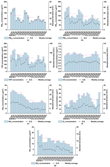
Figure 6.
Daily variations of mean concentrations for air pollutants in Xiangyang from a week before Chinese New Year to a week after Chinese New Year: (a) PM2.5; (b) PM10; (c) TSP; (d) CO; (e) NO2; (f) O3; (g) SO2.
3.3.3. Day-of-Week Characteristics
Large cohort studies have investigated on the day-of-week variation by averaging every Monday to Sunday concentration for each air pollutant during the studied period, and they found that the mean concentration of a weekday (such as Wednesday) was higher than that of a weekend day (Saturday or Sunday) [15,17,19,20]. In our study, to clarify whether pollution concentrations are significantly heavier during weekdays than those during weekends, we performed the Kruskal-Wallis test at the significant level of 5% and the null hypothesis () is no significant differences of distributions of air pollutants during holidays and non-holiday period. It can be seen from the Table 6 that all p values of the difference test are larger than 0.05, suggesting no significant weekday-weekend statistical difference in Xiangyang during the studied period. That is to say, unclear weekend effect for all air pollutants during the studied period is confirmed.
Table 6.
Results of weekday-weekend statistical difference tests at 16 measurement stations.
3.3.4. Diurnal Characteristics
Diurnal variations of air pollutants are shown in Figure 7. The diurnal characteristics of CO remain at a relatively steady status, despite two slight growths linked to the morning and evening rush hours. PM2.5, PM10, TSP, NO2 and SO2 enjoy similar diurnal characteristics with traffic-related double uptrends (5:00–8:00 and 17:00–20:00), and one downtrend (9:00–17:00), mainly ascribed to the change of PBLH. According to prior studies, the normal distributed PBLH increases from early in the morning (around 5:00 a.m.) to the noon, and then decreases to the minimum at night [14,19]. That is to say, the alleviated pollutant burden from noon to the afternoon results in the growth of PBLH by providing more volume to disperse pollutants. However, the decreases are not as drastic as expected. One possible reason for that is the counteractive effect of a synchronous decline of RH (Figure 7), which has adverse impacts on getting particles together to deposit. From the evening to the next day sunrise, lower PBLH enhances the concentrations of those pollutants, spontaneously leading to a high level of overnight pollution concentration, despite less anthropogenic emissions during that period. Interestingly, the diurnal variation of O3 concentration exhibits a thoroughly reverse pattern with a dramatic increase from 9:00 to 17:00, followed by a pronounced decrease persisting until the next day morning. Higher temperature at noon and in the afternoon (Figure 7) provides favorable conditions for photochemical activities accompanied by consumptions of NO2 and CO to generate O3. Furthermore, tails (20:00–23:00) of particulate trends vary from each other: (1) PM2.5 concentration gradually drops; (2) PM10 concentration maintains a stable condition; (3) TSP continues its growth till the next day morning. The on-road diesel trucks are permitted to transport construction waste from 22:00 to midnight according to relevant governmental regulations [36] and they contribute to the abundance of coarse particles accompanied by six-fold emissions more than those of other vehicles [14,45].
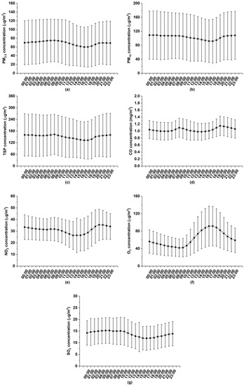
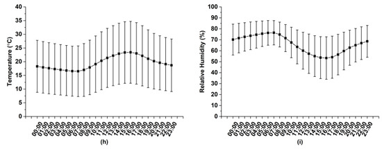
Figure 7.
Daily variations of mean values of air pollutants, temperature and relative humidity in Xiangyang from March 1, 2018 to February 28, 2019: (a) PM2.5; (b) PM10; (c) TSP; (d) CO; (e) NO2; (f) O3; (g) SO2; (h) temperature; (i) relative humidity (The bars indicate mean value ± standard deviation).
3.4. Relationships between Air Pollutants and Meteorological Parameters
Figure 8 illustrates the relationships between seven air pollutants and three meteorological parameters. Generally, all correlation coefficients here are relatively lower than reported in previous studies, which could be caused by three possible reasons. The first reason can be different time resolutions between the data of air pollutants (hourly) and meteorological parameters (daily) in previous studies. The second reason is that air pollutants and meteorological parameters for the same city are measured by different stations situated at different locations. The last reason can be the nonlinear relationship between the studied air pollutants and meteorological parameters. RH positively correlates with PM2.5 in all seasons while showing evident season-changed (i.e., negative in spring and summer, positive in winter and autumn) correlations with coarse particles (i.e., PM10 and TSP). In warm seasons (i.e., spring and summer), a relatively larger amount of precipitation is reported, suggesting higher RH, and then the degree of wet deposition for hygroscopic particles is aggravated under such damp weathers, inducing the reduction of PM10 and TSP. Given the fact that RH positively correlates with PM2.5 in all seasons, we assert that RH does not play an evident role in scavenging fine particles. Nevertheless, a different mechanism is set up in cold seasons. Normally, RH is closely associated with aerosols in winter and autumn, helping aerosol precursors convert to secondary aerosol, which in turn magnifies the concentration of PM2.5 [19,46,47]. This also explains the relatively higher correlation coefficient between RH and PM2.5 than those between RH and coarse particles. As for the correlation coefficients of temperature with particulate pollutants, negative correlation coefficients appear from June to October (without July) and positive correlation coefficients display since November until February of the next year. The negative correlation correlations are due to better dispersion as well as wet deposition by the joint effect of more precipitations, stronger wind, thicker PBLH and better vertical air mixing.
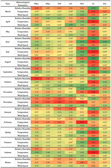
Figure 8.
Spearman’s correlation coefficients between air pollutants and meteorological parameters. (All correlations are significant at 99% confidence interval. a Correlations are not significant. b Correlations are significant at 95% confidence interval. The darker the red, the stronger positive correlation and the darker the green, the stronger negative correlation.)
In cold seasons, on the one hand, particles can take advantage of meteorological characteristics to accumulate, and on the other, enhanced secondary particulate pollutants, involving SO2 consumption, are generated and further sustained by the positive correlation between temperature and SO2 in some months. Moreover, higher temperature is beneficial to photochemical reactions. Therefore, temperature positively correlates with O3, especially in warm seasons, while negatively correlates with CO. Lower temperature and less sunlight inevitably hamper the evaporation effect, and therefore bring higher RH.
This probably explains the relatively stronger positive correlation coefficients of RH with CO and with SO2 during those seasons. The variability of the correlation between temperature and NO2 lies in the complex mechanism between NO2 and O3 in different meteorological characteristics. That is to say, the formation of secondary O3 by processing NO2 is relatively stronger in spring and summer while the oxidation from NOx to NO2 is relatively stronger in autumn and winter. In terms of WS, all air pollutants, excluding O3, display inverse correlations in most months, due to the higher WS the better dispersion of pollutants. Furthermore, among all correlations between WS and particulate pollutants, the correlations with coarse particles are relatively weaker, probably due to dust resuspended by the wind. Yet, the strong positive correlation with O3 may result in regional transported O3 [48]. Notably, the correlation coefficients of WS with all air pollutants here are relatively lower than those of previous studies [18,19,23]. Apart from a possibility of the nonlinear relationship, another possible reason is different WS measurements between our study and previous studies. Specifically, the WS applied in our study is of street-level wind which is remarkably slowed down by high-density infrastructures in the built environment while the WS used in previous studies is of urban wind, despite similarities in fluctuations (Figure 9).
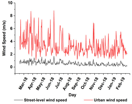
Figure 9.
Comparisons of monthly mean variations for street-level wind speed (collected by 16 measurement station) and urban wind speed (collected by the China Meteorology Administration) from 1 March 2018 to 28 February 2019.
3.5. Implications and Limitations
Like Xiangyang, many prefecture-level cities whose GDP mainly relies on industrial production are confronting potent hazy weather as much as key cities. However, limited attention has been paid to this phenomenon. Therefore, our study seeks to provide a holistic and systematical examination of the spatiotemporal variations of both particulate and gaseous pollutants as well as on their relations to meteorological parameters for prefecture-level cities, which can be fully used by policy-makers to take accurate measures to mitigate the haze problem. Meanwhile, we reasonably demonstrated that it is imperative that air pollutants and meteorological parameters be synchronously monitored through ground measurements. Furthermore, this all-sided study can fill in the gap in the field of spatiotemporal variations of air pollutants at an urban scale. Nevertheless, our study has some limitations. First, one-year measurements are insufficient for analyses of seasonal variations and holiday effect, as longer time span measurements can rule out some uncertainties. Second, some meteorological factors, such as precipitations, sunshine durations and the PBLH, have not been participated in the Spearman’s rank correlation coefficient test in our study as unable to be synchronously measured by those 16 stations. Nevertheless, they can directly and indirectly disrupt the pollution concentration that was demonstrated by other studies [21,49,50,51,52]. Therefore, more monitoring parameters of ground stations and a precise measurement of PBLH for Xiangyang are well needed. Finally, further investigations on whether the relationship between the studied air pollutants and meteorological parameters is nonlinear or not are requested.
4. Conclusions
In this paper, we analyzed the spatiotemporal variations of particulate and gaseous pollutants and their relations to meteorological parameters in Xiangyang, China, from 1 March 2018 to 28 February 2019. The principal conclusions are as follows:
- (1)
- The percentage of the days with excellent and good air quality (64.6%) fails to reach the criteria of 80% proposed by China’s 13th Five-Year Plan (2016–2020). PM2.5, O3 and PM10 are the main primary pollutants. Moreover, PM2.5 and PM10 act as primary pollutants all the year round and O3 loses its primary pollutant position after November.
- (2)
- Annual concentrations of PM2.5 and PM10 of all stations strikingly exceed both the CNAAQS and WHOAQG. The largest abundance of gaseous pollutants is identically from Station 15, surrounded by nine chemical plants while the maximal enhancement of particulate pollutants is observed at Station 6, ascribed to its land use for automobile manufacture. TSP concentration is closely related to on-going construction sites but can be alleviated by road sprinkler operations.
- (3)
- A distinct seasonal trend for “worse winter and better summer” is unveiled. However, the concentration of CO maintains a relatively stable condition in the whole year. Concentrations of PM2.5, PM10, TSP, NO2 and SO2 enjoy similar two traffic-related uptrends (5:00–8:00 and 17:00–20:00) and one downtrend (9:00–17:00), while the concentration of O3 fluctuates oppositely due to photochemical reactions.
- (4)
- An unclear weekend effect is confirmed for all pollutants. Significant differences of NO2 and SO2 during NDH and non-NDH as well as significant differences of NO2 and O3 during CNY and non-CNY are unveiled. Celebration activities for CNY bring distinctly increased concentrations of SO2 and secondary particulate pollutants.
- (5)
- RH positively correlates with PM2.5 in all seasons while showing evident season-changed (i.e., negative in spring and summer, positive in winter and autumn) correlations with coarse particles. Positive correlation coefficients of temperature with O3 appear in all seasons, and positive correlation coefficients of temperature with all other pollutants are shown only in winter. WS positively correlates with O3 while negatively correlates with the rest.
In the future, quantitative efforts to clarify the air pollution distribution in the built environment, and simultaneously to take into consideration with more urban features such as building density, percentage of greenery coverage, etc. need to be made.
Author Contributions
W.X. conceived and designed the framework, performed data preprocessing and analyses as well as composed the manuscript; Q.Z. (Qingming Zhan) managed the project and edited the manuscript; Q.Z. (Qi Zhang) participated in the data preprocessing and edited the manuscript; Z.W. collected the measurement data and conducted the field interview. All authors have read and agreed to the published version of the manuscript.
Funding
This work was funded by the National Natural Science Foundation of China under Grant No. 51878515.
Acknowledgments
We would like to acknowledge the Xiangyang Environmental Monitoring Center, the Xiangyang Natural Resources and Planning Bureau, the Google Map team, the Xiangyang Housing and Urban-Rural Development Bureau and the China Meteorological Administration for the data used in this paper.
Conflicts of Interest
The authors declare no conflict of interest.
References
- Xie, Y.; Zhao, B.; Zhang, L.; Luo, R. Spatiotemporal variations of PM2.5 and PM10 concentrations between 31 Chinese cities and their relationships with SO2, NO2, CO and O3. Particuology 2015, 20, 141–149. [Google Scholar] [CrossRef]
- Cohen, A.J.; Brauer, M.; Burnett, R.; Anderson, H.R.; Frostad, J.; Estep, K.; Balakrishnan, K.; Brunekreef, B.; Dandona, L.; Dandona, R.; et al. Estimates and 25-year trends of the global burden of disease attributable to ambient air pollution: An analysis of data from the Global Burden of Diseases Study 2015. Lancet 2017, 389, 1907–1918. [Google Scholar] [CrossRef]
- World Health Organization. World Health Statistics 2018: Monitoring Health for the SDGs; WHO: Geneva, Switzerland, 2018; p. 39. ISBN 978-92-4-156558-5. [Google Scholar]
- Lelieveld, J.; Evans, J.S.; Fnais, M.; Giannadaki, D.; Pozzer, A. The contribution of outdoor air pollution sources to premature mortality on a global scale. Nature 2015, 525, 367–371. [Google Scholar] [CrossRef] [PubMed]
- Zou, B.; You, J.; Lin, Y.; Duan, X.; Zhao, X.; Fang, X.; Campen, M.J.; Li, S. Air pollution intervention and life-saving effect in China. Environ. Int. 2019, 125, 529–541. [Google Scholar] [CrossRef]
- Wu, R.; Song, X.; Chen, D.; Zhong, L.; Huang, X.; Bai, Y.; Hu, W.; Ye, S.; Xu, H.; Feng, B.; et al. Health benefit of air quality improvement in Guangzhou, China: Results from a long time-series analysis (2006–2016). Environ. Int. 2019, 126, 552–559. [Google Scholar] [CrossRef]
- Jerrett, M.; Burnett, R.T.; Pope, C.A.; Ito, K.; Thurston, G.; Krewski, D.; Shi, Y.; Calle, E.; Thun, M. Long-Term Ozone Exposure and Mortality. N. Engl. J. Med. 2009, 360, 1085–1095. [Google Scholar] [CrossRef]
- Bernard, S.M.; Samet, J.M.; Grambsch, A.; Ebi, K.L.; Romieu, I. The potential impacts of climate variability and change on air pollution-related health effects in the United States. Environ. Health Perspect. 2001, 109, 199–209. [Google Scholar] [CrossRef]
- Clark, N.A.; Demers, P.A.; Karr, C.J.; Koehoorn, M.; Lencar, C.; Tamburic, L.; Brauer, M. Effect of early life exposure to air pollution on development of childhood asthma. Environ. Health Perspect. 2010, 118, 284–290. [Google Scholar] [CrossRef]
- Hu, J.; Wang, Y.; Ying, Q.; Zhang, H. Spatial and temporal variability of PM2.5 and PM10 over the North China Plain and the Yangtze River Delta, China. Atmos. Environ. 2014, 95, 598–609. [Google Scholar] [CrossRef]
- Li, J.; Han, X.; Li, X.; Yang, J.; Li, X. Spatiotemporal Patterns of Ground Monitored PM(2.5) Concentrations in China in Recent Years. Int. J. Environ. Res. Public Health 2018, 15, 114. [Google Scholar] [CrossRef]
- Lin, Y.; Zou, J.; Yang, W.; Li, C.-Q. A Review of Recent Advances in Research on PM2.5 in China. Int. J. Environ. Res. Public Health 2018, 15, 438. [Google Scholar] [CrossRef] [PubMed]
- Chan, C.K.; Yao, X. Air pollution in mega cities in China. Atmos. Environ. 2008, 42, 1–42. [Google Scholar] [CrossRef]
- Zhang, Y.-L.; Cao, F. Fine particulate matter (PM2.5) in China at a city level. Sci. Rep. 2015, 5, 14884. [Google Scholar] [CrossRef] [PubMed]
- Li, Y.; Dai, Z.; Liu, X. Analysis of Spatial-Temporal Characteristics of the PM2.5 Concentrations in Weifang City, China. Sustainability 2018, 10, 2960. [Google Scholar] [CrossRef]
- Zhao, X.; Gao, Q.; Sun, M.; Xue, Y.; Ma, R.; Xiao, X.; Ai, B. Statistical Analysis of Spatiotemporal Heterogeneity of the Distribution of Air Quality and Dominant Air Pollutants and the Effect Factors in Qingdao Urban Zones. Atmosphere 2018, 9, 135. [Google Scholar] [CrossRef]
- Yao, L.; Lu, N.; Yue, X.; Du, J.; Yang, C. Comparison of Hourly PM2.5 Observations Between Urban and Suburban Areas in Beijing, China. Int. J. Environ. Res. Public Health 2015, 12, 12264–12276. [Google Scholar] [CrossRef] [PubMed]
- Chen, T.; He, J.; Lu, X.; She, J.; Guan, Z. Spatial and Temporal Variations of PM2.5 and Its Relation to Meteorological Factors in the Urban Area of Nanjing, China. Int. J. Environ. Res. Public Health 2016, 13, 921. [Google Scholar] [CrossRef]
- Liu, Z.; Hu, B.; Wang, L.; Wu, F.; Gao, W.; Wang, Y. Seasonal and diurnal variation in particulate matter (PM10 and PM2.5) at an urban site of Beijing: Analyses from a 9-year study. Environ. Sci. Pollut. Res. Int. 2015, 22, 627–642. [Google Scholar] [CrossRef]
- Chai, F.; Gao, J.; Chen, Z.; Wang, S.; Zhang, Y.; Zhang, J.; Zhang, H.; Yun, Y.; Ren, C. Spatial and temporal variation of particulate matter and gaseous pollutants in 26 cities in China. J. Environ. Sci. 2014, 26, 75–82. [Google Scholar] [CrossRef]
- Yin, X.; de Foy, B.; Wu, K.; Feng, C.; Kang, S.; Zhang, Q. Gaseous and particulate pollutants in Lhasa, Tibet during 2013–2017: Spatial variability, temporal variations and implications. Environ. Pollut. 2019, 253, 68–77. [Google Scholar] [CrossRef]
- DeGaetano, A.T.; Doherty, O.M. Temporal, spatial and meteorological variations in hourly PM2.5 concentration extremes in New York City. Atmos. Environ. 2004, 38, 1547–1558. [Google Scholar] [CrossRef]
- Zhang, H.; Wang, Y.; Hu, J.; Ying, Q.; Hu, X.-M. Relationships between meteorological parameters and criteria air pollutants in three megacities in China. Environ. Res. 2015, 140, 242–254. [Google Scholar] [CrossRef] [PubMed]
- Tan, P.-H.; Chou, C.; Liang, J.-Y.; Chou, C.C.K.; Shiu, C.-J. Air pollution “holiday effect” resulting from the Chinese New Year. Atmos. Environ. 2009, 43, 2114–2124. [Google Scholar] [CrossRef]
- Xu, W.; Tian, Y.; Liu, Y.; Zhao, B.; Liu, Y.; Zhang, X. Understanding the Spatial-Temporal Patterns and Influential Factors on Air Quality Index: The Case of North China. Int. J. Environ. Res. Public Health 2019, 16, 2820. [Google Scholar] [CrossRef] [PubMed]
- Xiangyang City Bureau of Statistics. Xiangyang Statistical Yearbook 2018. Available online: http://tjj.xiangyang.gov.cn/tjsj/sjcx/tjnb/201901/P020190124423422545825.pdf (accessed on 8 August 2019).
- Ministry of Ecology and Environment of China. Ambient Air Quality Standards. Available online: http://kjs.mee.gov.cn/hjbhbz/bzwb/dqhjbh/dqhjzlbz/201203/W020120410330232398521.pdf (accessed on 8 August 2019).
- Standardization Administration of the P.R.C. Specifications for Surface Meteorological Observation-Air Temperature and Humidity. Available online: http://c.gb688.cn/bzgk/gb/showGb?type=online&hcno=FF9A1553D415BA3D6B05340DDC0B49A2 (accessed on 8 August 2019).
- Standardization Administration of the P.R.C. Specifications for Surface Meteorological Observation-Wind Direction and Wind Speed. Available online: http://c.gb688.cn/bzgk/gb/showGb?type=online&hcno=F8D676CA723CDDB7597E9BBACD404891 (accessed on 8 August 2019).
- Ministry of Ecology and Environment of China. Technical Specifications for Installation and Acceptance of Ambient Air Quality Continuous Automated Monitoring System for PM10 and PM2.5. Available online: http://kjs.mee.gov.cn/hjbhbz/bzwb/jcffbz/201308/W020130802492823718666.pdf (accessed on 8 August 2019).
- Ministry of Ecology and Environment of China. Technical Specifications for Installation and Acceptance of Ambient air Quality Continuous Automated Monitoring System for SO2, NO2, O3 and CO. Available online: http://kjs.mee.gov.cn/hjbhbz/bzwb/jcffbz/201308/W020130802493970989627.pdf (accessed on 8 August 2019).
- The China Meteorological Data Service Center. Data Access-Surface. Available online: http://data.cma.cn/en/?r=data (accessed on 8 August 2019).
- Tong, Z.; Chen, Y.; Malkawi, A.; Liu, Z.; Freeman, R.B. Energy saving potential of natural ventilation in China: The impact of ambient air pollution. Appl. Energy 2016, 179, 660–668. [Google Scholar] [CrossRef]
- Liu, H.; Fang, C.; Zhang, X.; Wang, Z.; Bao, C.; Li, F. The effect of natural and anthropogenic factors on haze pollution in Chinese cities: A spatial econometrics approach. J. Clean. Prod. 2017, 165, 323–333. [Google Scholar] [CrossRef]
- Ministry of Ecology and Environment of China. Technical Regulation on Ambient Air Quality Index (on trial). Available online: http://kjs.mee.gov.cn/hjbhbz/bzwb/jcffbz/201203/W020120410332725219541.pdf (accessed on 8 August 2019).
- Xiangyang Natural Resources and Planning Bureau. Openness in Governmental Affairs-Program Plannings. Available online: http://zrzygh.xiangyang.gov.cn/zwgk/gkml/?itemid=1877 (accessed on 24 September 2019).
- Xiangyang Housing and Urban-Rural Development Bureau. Openness in Governmental Affairs. Available online: http://szjj.xiangyang.gov.cn/zwgk/gkml/?itemid=2196 (accessed on 24 September 2019).
- Li, C.; Wang, Z.; Li, B.; Peng, Z.-R.; Fu, Q. Investigating the relationship between air pollution variation and urban form. Build. Environ. 2019, 147, 559–568. [Google Scholar] [CrossRef]
- Tian, Y.; Yao, X.; Chen, L. Analysis of spatial and seasonal distributions of air pollutants by incorporating urban morphological characteristics. Comput. Environ. Urban Syst. 2019, 75, 35–48. [Google Scholar] [CrossRef]
- Calderón, S.M.; Poor, N.D.; Campbell, S.W.; Tate, P.; Hartsell, B. Rainfall scavenging coefficients for atmospheric nitric acid and nitrate in a subtropical coastal environment. Atmos. Environ. 2008, 42, 7757–7767. [Google Scholar] [CrossRef]
- Tan, P.-H.; Chou, C.; Chou, C.C.K. Impact of urbanization on the air pollution “holiday effect” in Taiwan. Atmos. Environ. 2013, 70, 361–375. [Google Scholar] [CrossRef]
- Leibensperger, E.M.; Mickley, L.J.; Jacob, D.J.; Barrett, S.R.H. Intercontinental influence of NOx and CO emissions on particulate matter air quality. Atmos. Environ. 2011, 45, 3318–3324. [Google Scholar] [CrossRef]
- World Health Organization. Air Quality Guidelines—Global Update 2005: Particulate Matter, Ozone, Nitrogen Dioxide, and Sulfur Dioxide; WHO: Geneva, Switzerland, 2006; pp. 217–395. ISBN 92-890-2192-6. [Google Scholar]
- Zhan, D.; Kwan, M.-P.; Zhang, W.; Yu, X.; Meng, B.; Liu, Q. The driving factors of air quality index in China. J. Clean. Prod. 2018, 197, 1342–1351. [Google Scholar] [CrossRef]
- Westerdahl, D.; Wang, X.; Pan, X.; Zhang, K.M. Characterization of on-road vehicle emission factors and microenvironmental air quality in Beijing, China. Atmos. Environ. 2009, 43, 697–705. [Google Scholar] [CrossRef]
- Sun, Y.L.; Wang, Z.F.; Fu, P.Q.; Yang, T.; Jiang, Q.; Dong, H.B.; Li, J.; Jia, J.J. Aerosol composition, sources and processes during wintertime in Beijing, China. Atmos. Chem. Phys. 2013, 13, 4577–4592. [Google Scholar] [CrossRef]
- Gao, Y.; Zhang, M.; Liu, Z.; Wang, L.; Wang, P.; Xia, X.; Tao, M.; Zhu, L. Modeling the feedback between aerosol and meteorological variables in the atmospheric boundary layer during a severe fog–haze event over the North China Plain. Atmos. Chem. Phys. 2015, 15, 4279–4295. [Google Scholar] [CrossRef]
- Gao, D.; Xie, M.; Chen, X.; Wang, T.; Zhan, C.; Ren, J.; Liu, Q. Modeling the Effects of Climate Change on Surface Ozone during Summer in the Yangtze River Delta Region, China. Int. J. Environ. Res. Public Health 2019, 16, 1528. [Google Scholar] [CrossRef]
- Zhao, C.; Tie, X.; Lin, Y. A possible positive feedback of reduction of precipitation and increase in aerosols over eastern central China. Geophys. Res. Lett. 2006, 33. [Google Scholar] [CrossRef]
- Qian, Y.; Gong, D.; Fan, J.; Leung, L.R.; Bennartz, R.; Chen, D.; Wang, W. Heavy pollution suppresses light rain in China: Observations and modeling. J. Geophys. Res. Atmos. 2009, 114, D7. [Google Scholar] [CrossRef]
- Chen, T.; Deng, S.; Gao, Y.; Qu, L.; Li, M.; Chen, D. Characterization of air pollution in urban areas of Yangtze River Delta, China. Chin. Geogr. Sci. 2017, 27, 836–846. [Google Scholar] [CrossRef][Green Version]
- Zhao, B.; Liou, K.N.; Gu, Y.; He, C.; Lee, W.L.; Chang, X.; Li, Q.; Wang, S.; Tseng, H.L.R.; Leung, L.Y.R.; et al. Impact of buildings on surface solar radiation over urban Beijing. Atmos. Chem. Phys. 2016, 16, 5841–5852. [Google Scholar] [CrossRef]


© 2019 by the authors. Licensee MDPI, Basel, Switzerland. This article is an open access article distributed under the terms and conditions of the Creative Commons Attribution (CC BY) license (http://creativecommons.org/licenses/by/4.0/).