Spatio-Temporal Dynamics of Maize Potential Yield and Yield Gaps in Northeast China from 1990 to 2015

Abstract
1. Introduction
2. Data and Methods
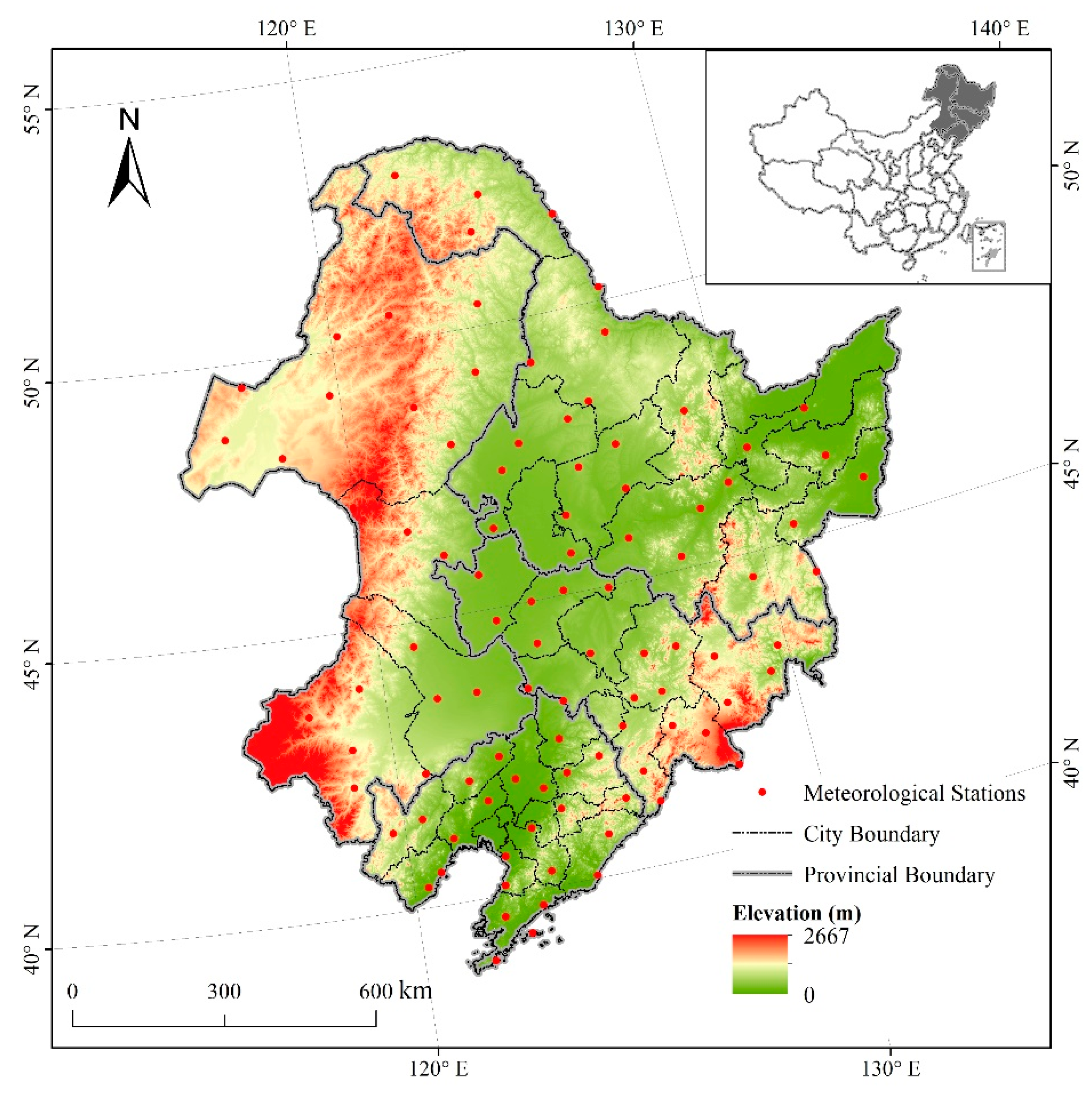
2.1. Study Area
2.2. Data Source
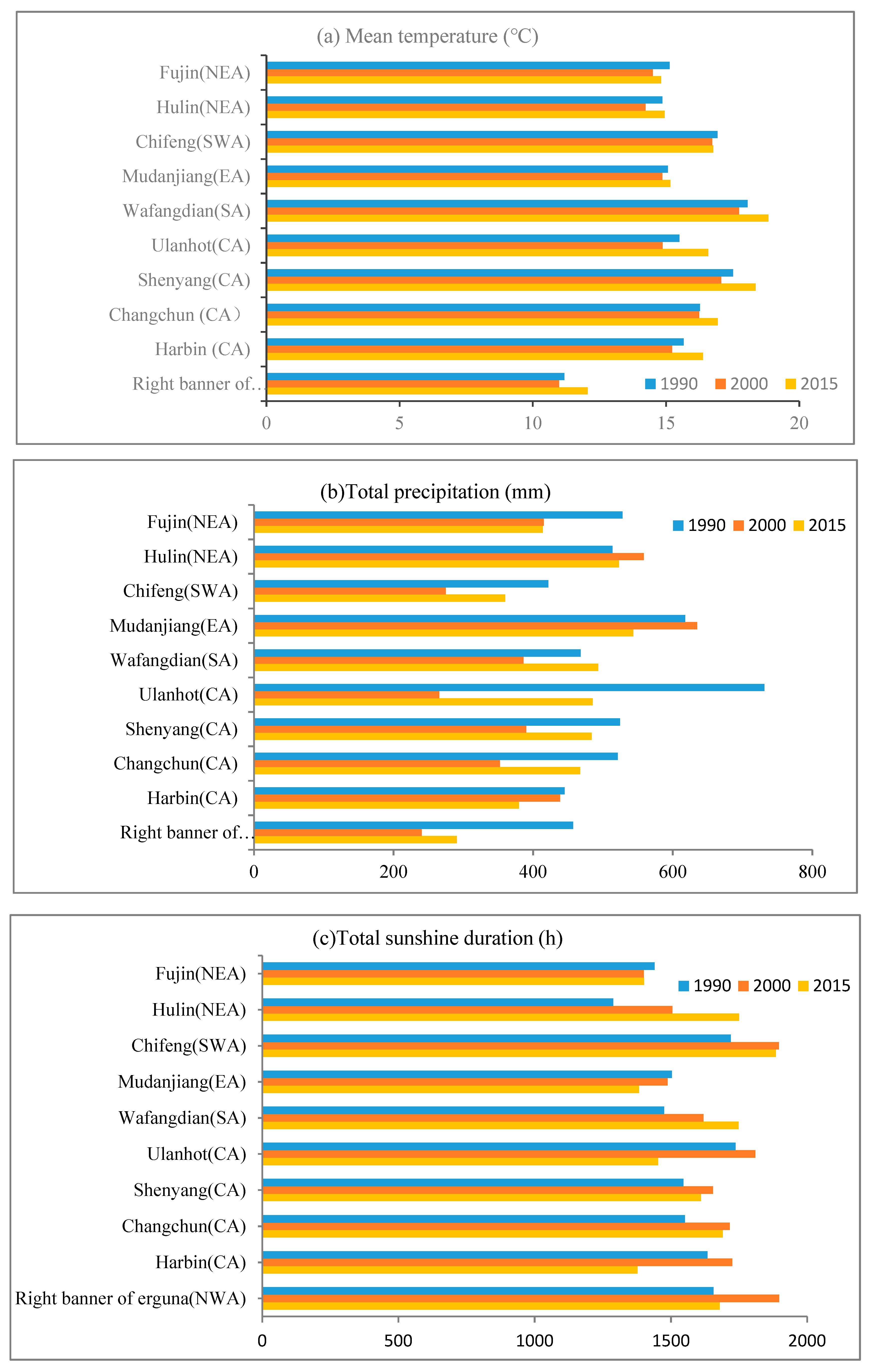
2.2.1. Input Data for the GAEZ Model
2.2.2. Other Data
2.3. Methods
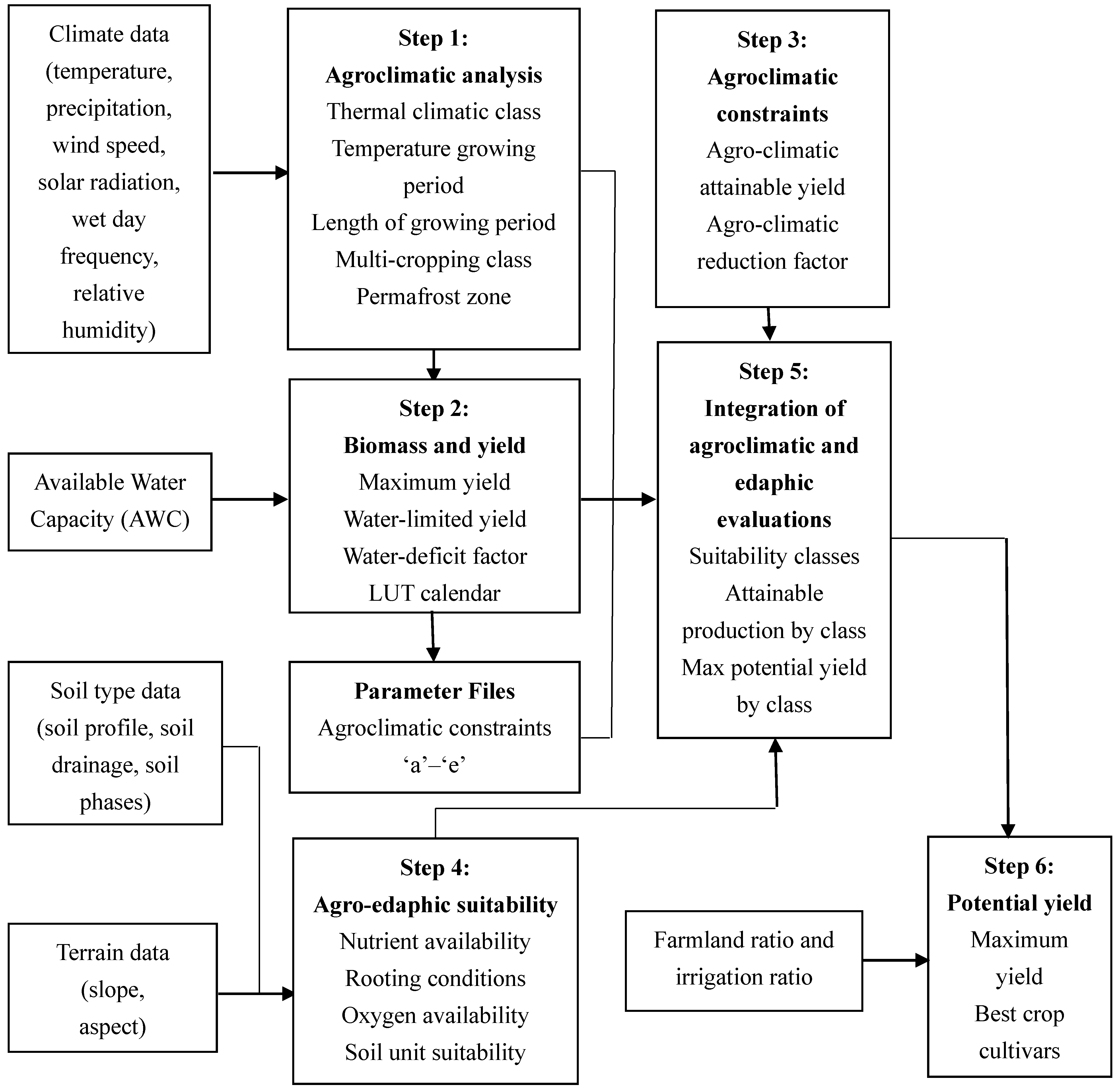
2.3.1. Procedures for Calculating Potential Yield
2.3.2. Spatio-Temporal Dynamics Analysis
2.3.3. Yield Gaps between Actual and Potential Yields
3. Results and Analysis
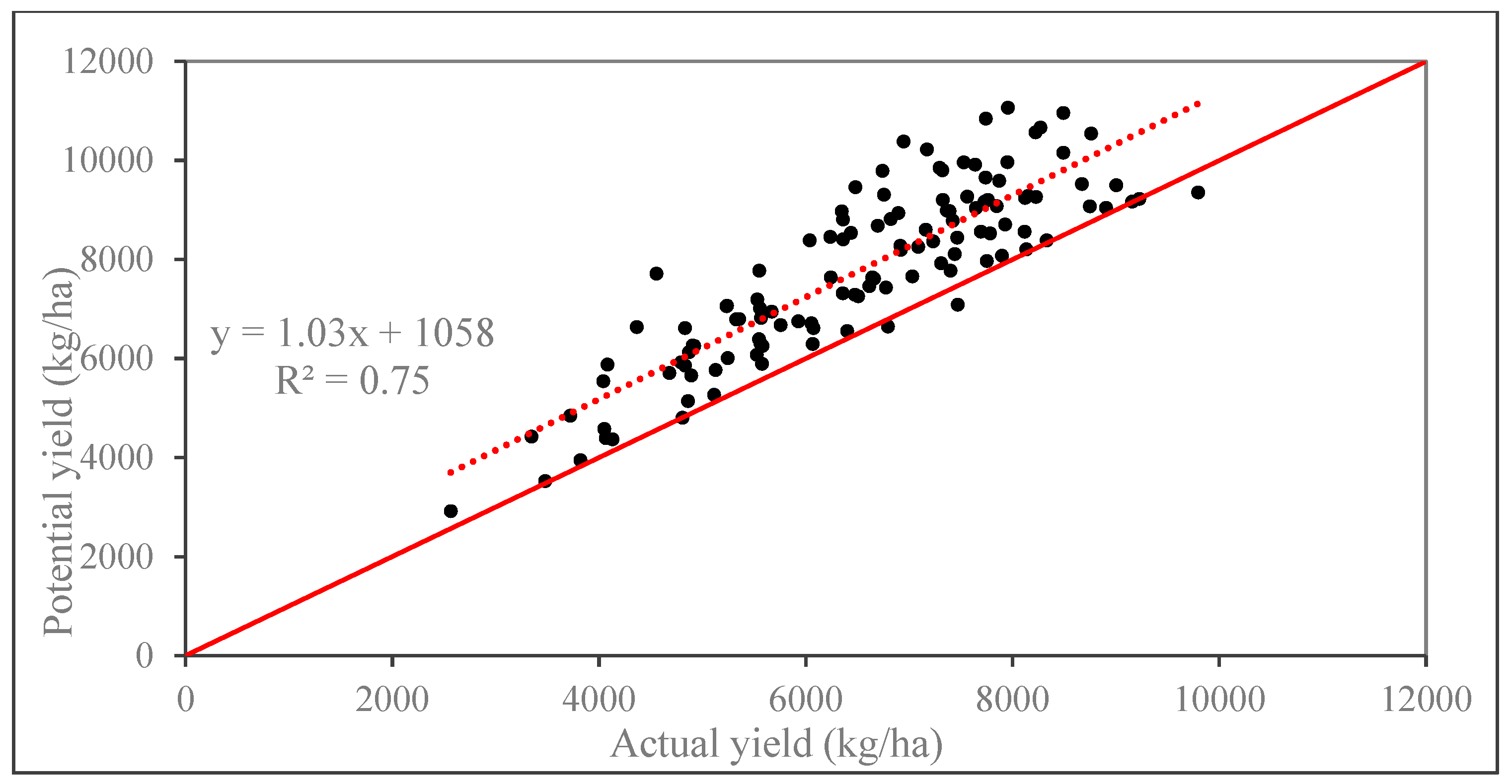
3.1. Validation of the GAEZ Model
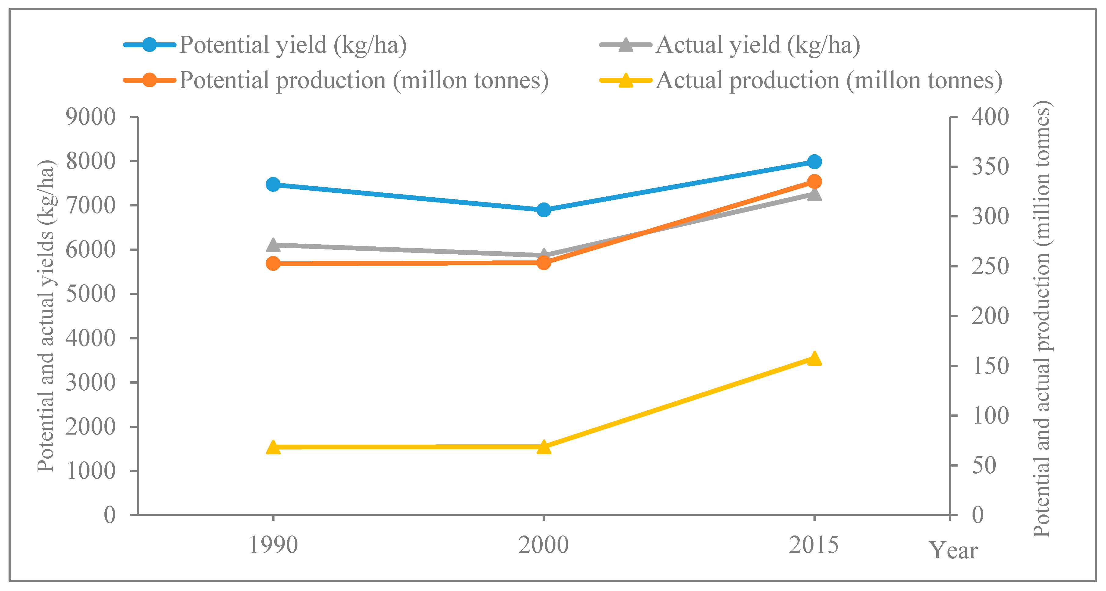
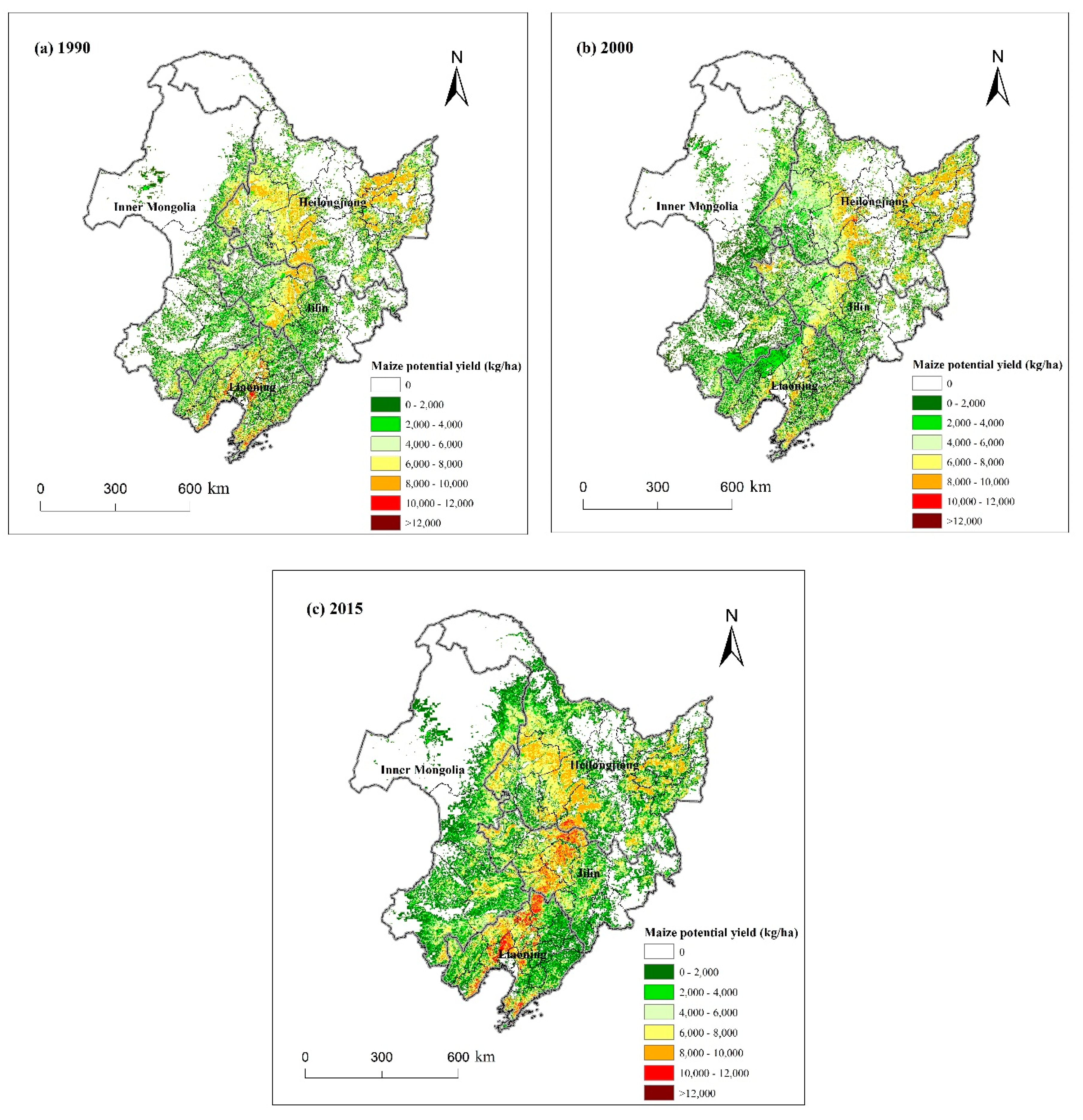
3.2. Temporal Change of Maize Potential Yield
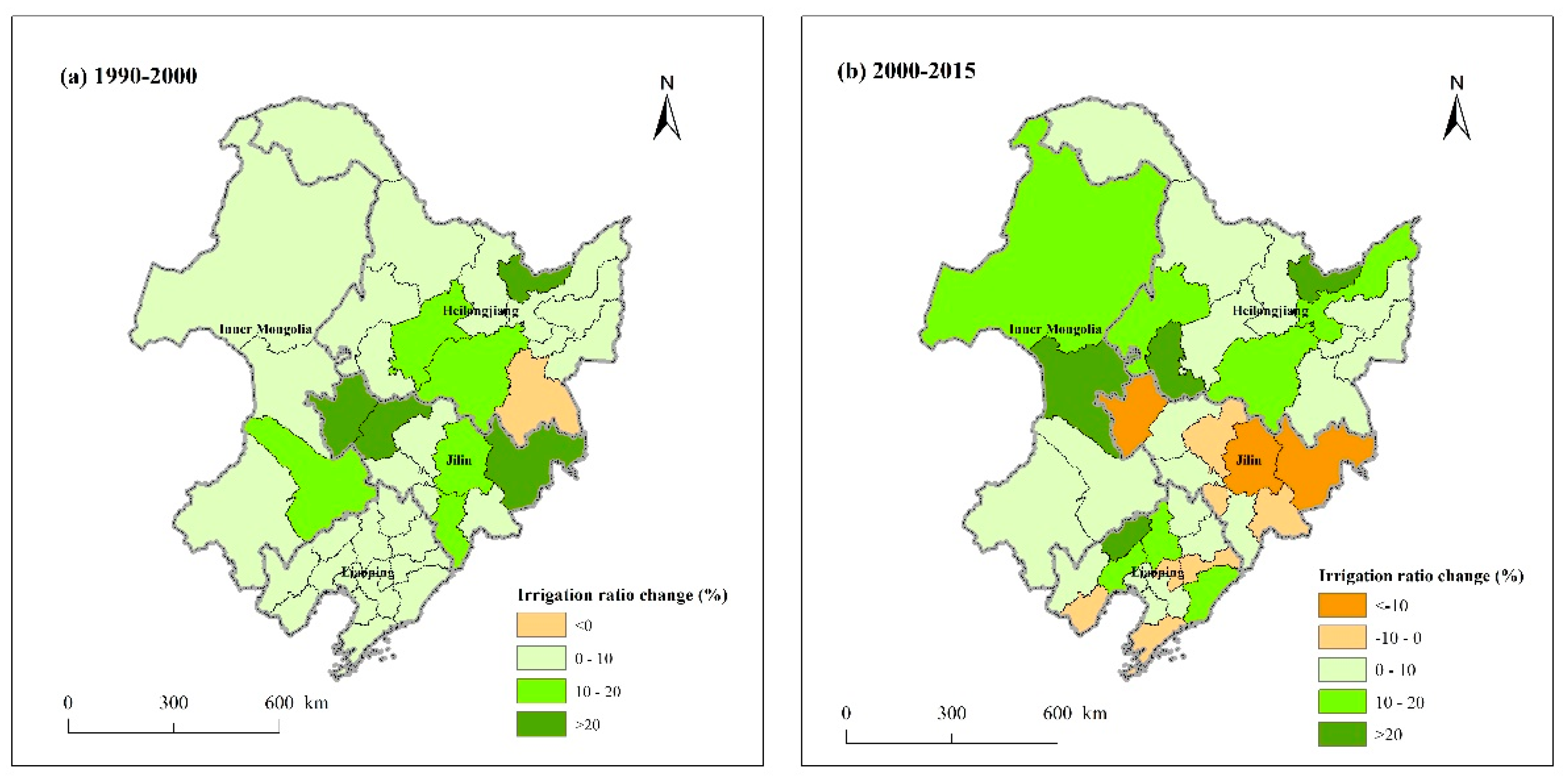
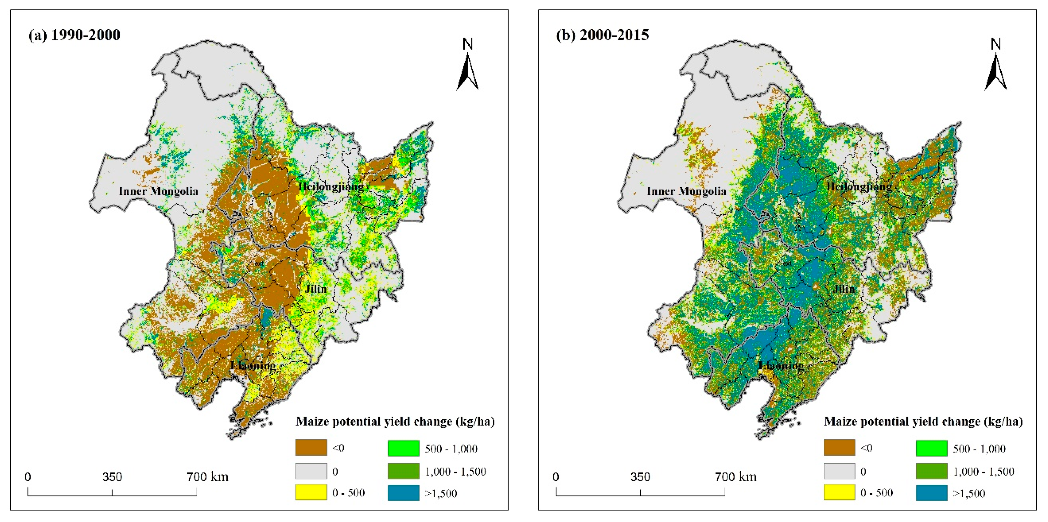
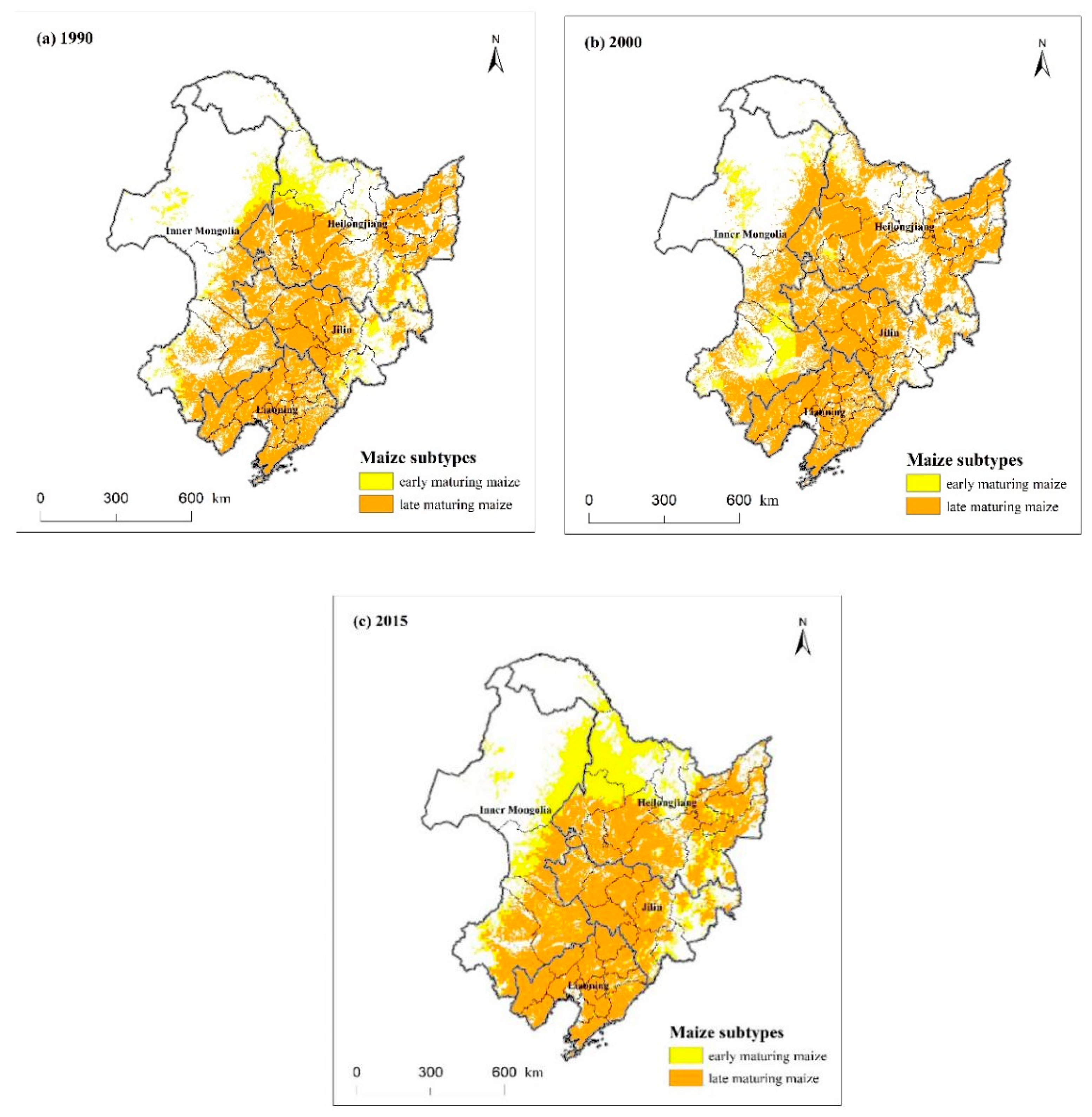
3.3. Spatial Dynamics of Maize Potential Yield
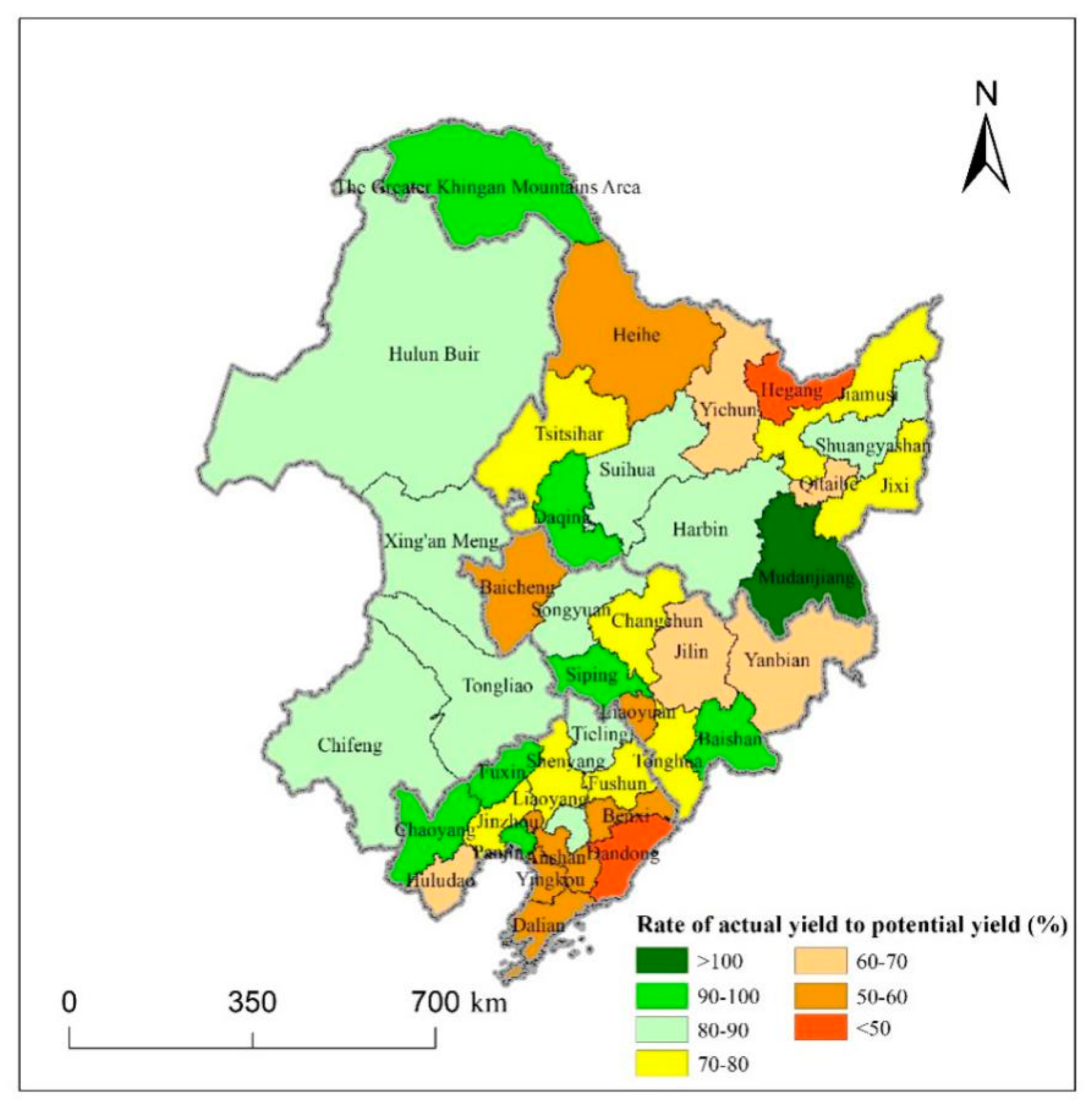
3.4. Yield Gaps between Actual and Potential Yields
4. Discussions
4.1. Limitations of Yield Gaps Analysis
4.2. Several Other Crop Production Models
4.3. The Advantages and Limitations of the GAEZ Model
5. Conclusions
Author Contributions
Acknowledgments
Conflicts of Interest
References
- Pingali, P. Westernization of Asian diets and the transformation of food systems: Implications for research and policy. Food Policy 2006, 32, 281–298. [Google Scholar] [CrossRef]
- Tilman, D.; Balzer, C.; Hill, J.; Befort, B. Global food demand and the sustainable intensification of agriculture. Proc. Natl. Acad. Sci. USA 2011, 108, 20260–20264. [Google Scholar] [CrossRef] [PubMed]
- Liu, Z. Maize potential yields and yield gaps in the changing climate of Northeast China. Glob. Chang. Biol. 2012, 18, 3441–3454. [Google Scholar] [CrossRef]
- Qin, Y.; Liu, J.; Shi, W.; Tao, F.; Yan, H. Spatial-temporal changes of cropland and climate potential productivity in Northern China during 1990–2010. Food Secur. 2013, 5, 499–512. [Google Scholar] [CrossRef]
- Zhang, Z.; Chen, Y.; Wang, P.; Zhang, S.; Tao, F.; Liu, X. Spatial and temporal changes of agro-meteorological disasters affecting maize production in China since 1990. Nat. Hazards 2014, 71, 2087–2100. [Google Scholar] [CrossRef]
- Ji, R.; Zhang, Y.; Jiang, L.; Zhang, S.; Feng, R.; Chen, P.; Wu, J.; Mi, N. Effect of climate change on maize production in Northeast China. Geogr. Res. 2012, 31, 290–298. [Google Scholar]
- Tao, F.; Zhang, S.; Zhang, Z.; Reimund, P. Temporal and spatial changes of maize yield potentials and yield gaps in the past three decades in China. Agric. Ecosyst. Environ. 2015, 208, 12–20. [Google Scholar] [CrossRef]
- Licker, R.; Johnston, M.; Foley, J.; Barford, C.; Kucharik, C.; Monfreda, C.; Ramankutty, N. Mind the gap: How do climate and agricultural management explain the ‘yield gap’ of croplands around the world? Glob. Ecol. Biogeogr. 2010, 19, 769–782. [Google Scholar] [CrossRef]
- Mueller, N.; Gerber, J.; Johnston, M.; Ray, D.; Ramankutty, N.; Foley, J. Closing yield gaps through nutrient and water management. Nature 2012, 490, 254–257. [Google Scholar] [CrossRef]
- Wang, J.; Wang, E.; Yin, H.; Feng, L.; Zhang, J. Declining yield potential and shrinking yield gaps of maize in the North China Plain. Agric. For. Meteorol. 2014, 195–196, 89–101. [Google Scholar] [CrossRef]
- Meng, Q.; Hou, P.; Wu, L.; Chen, X.; Cui, Z.; Zhang, F. Understanding production potentials and yields gaps in intensive maize production in China. Field Crops Res. 2013, 143, 91–97. [Google Scholar] [CrossRef]
- Grassini, P.; Yang, H.; Cassman, K. Limits to maize productivity in Western Corn-Belt: A simulation analysis for fully irrigated and rainfed conditions. Agric. For. Meteorol. 2009, 149, 1254–1265. [Google Scholar] [CrossRef]
- Du, G.; Zhang, L.; Xu, X.; Wang, J. Spatial-temporal characteristics of maize production potential change under the background of climate change in Northeast China over the past 50 years. Geogr. Res. 2016, 35, 864–874. [Google Scholar]
- Mao, D.; Wang, Z.; Luo, L.; Ren, C. Integrating AVHRR and MODIS data to monitor NDVI changes and their relationships with climatic parameters in Northeast China. Int. J. Appl. Earth Obs. Geo Inf. 2012, 18, 528–536. [Google Scholar] [CrossRef]
- Gao, G.; Jie, D.; Wang, Y.; Liu, L.; Liu, H.; Li, D.; Li, N.; Shi, J.; Leng, C. Do soil phytoliths accurately represent plant communities in a temperate region? A case study of Northeast China. Veg. Hist. Archaeobotany. 2018, 27, 753–765. [Google Scholar] [CrossRef]
- Tan, J.; Li, Z.; Yang, P.; Liu, Z.; Zhang, L.; Wu, W.; You, L.; Tang, H. Spatio-temporal changes of maize sown area and yield in Northeast China between 1980 and 2010 using spatial production allocation model. Acta Geogr. Sin. 2014, 69, 353–364. [Google Scholar]
- Zhao, G.; Wang, J.; Fan, W.; Ying, T. Vegetation net primary productivity in Northeast China in 2000–2008: Simulation and seasonal change. Chin. J. Appl. Ecol. 2011, 22, 621. [Google Scholar]
- Sun, X.; Ren, B.; Zhuo, Z.; Gao, C.; Zhou, G. Faunal composition of grasshopper in different habitats of Northeast China? Chin. J. Ecol. 2006, 25, 286–289. [Google Scholar]
- Jilin Statistical Yearbook (1984–2017); Statistical Bureau of Jilin: Jilin, China, 2018.
- Liaoning Statistical Yearbook (1983–2017); Statistical Bureau of Liaoning: Liaoning, China, 2018.
- Heilongjiang Statistical Yearbook (1985–2017); Statistical Bureau of Heilongjiang: Heilongjiang, China, 2018.
- Inner Mongolia Statistical Yearbook (1985–2018); Statistical Bureau of Inner Mongolia: Inner Mongolia, China, 2019.
- Hutchinson, M. Interpolating mean rainfall using thin plate smoothing splines. Int. J. Geogr. Inf. Syst. 1995, 9, 385–403. [Google Scholar] [CrossRef]
- Hutchinson, M. Interpolation of rainfall data with thin plate smoothing splines. Part I: Two dimensional smoothing of data with short range correlation. J. Geogr. Inf. Decis. Anal. 1998, 2, 139–151. [Google Scholar]
- Hutchinson, M. Interpolation of rainfall data with thin plate smoothing splines. Part II: Analysis of topographic dependence. J. Geogr. Inf. Decis. Anal. 1998, 2, 152–167. [Google Scholar]
- Yuji, M.; Kiyoshi, T.; Hideo, H.; Yuzuru, M. Impact assessment of climate change on rice production in Asia in comprehensive consideration of process/parameter uncertainty in general circulation models. Agric. Ecosyst. Environ. 2009, 131, 281–291. [Google Scholar]
- Shortridge, A.; Messina, J. Spatial structure and landscape associations of SRTM error. Remote Sens. Environ. 2011, 115, 1576–1587. [Google Scholar] [CrossRef]
- Tian, Z.; Zhong, H.; Sun, L.; Fischer, G.; Velthuizen, H.; Liang, Z. Improving performance of Agro-Ecological Zone (AEZ) modeling by cross-scale model coupling: An application to japonica rice production in Northeast China. Ecol. Model. 2014, 290, 155–164. [Google Scholar] [CrossRef]
- Pu, L.; Zhang, S.; Li, F.; Wang, R.; Yang, J.; Chang, L. Impact of farmland change on soybean production potential in recent 40 years: A case study in Western Jilin, China. Int. J. Environ. Res. Public Health 2018, 15, 1522. [Google Scholar] [CrossRef]
- Smith, M. CROPWAT: A Computer Program for Irrigation Planning and Managemen; Food & Agriculture Organization of the United Nations: Roma, Italy, 1992. [Google Scholar]
- Monteith, J. Evaporation and surface temperature. Q. J. R. Meteorol. Soc. 1981, 107, 1–27. [Google Scholar] [CrossRef]
- Fischer, G.; Velthuizen, H.; Shah, M.; Nachtergaele, F. Global agro-ecological assessment for agriculture in the 21st century. J. Henan Vocat.-Tech. Teach. Coll 2002, 11, 371–374. [Google Scholar]
- Tatsumi, K.; Yamashiki, Y.; Valmir da Silva, R.; Takara, K.; Matsuoka, Y.; Takahashi, K.; Maruyama, K.; Kawahara, N. Estimation of potential changes in cereals production under climate change scenarios. Hydrol. Process 2011, 25, 2715–2725. [Google Scholar] [CrossRef]
- Stehfest, E.; Heistermann, M.; Priess, J.; Ojima, D.; Alcamo, J. Simulation of global crop production with the ecosystem model DayCent. Ecol. Model. 2007, 209, 203–219. [Google Scholar] [CrossRef]
- Williams, J.; Jones, C.; Dyke, P. The EPIC model and its application Process. In Proceedings of the International Symposium on Minimum Data Sets for Agrotechnology Transfer, Patancheru, India, 21–26 March 1984; pp. 111–121. [Google Scholar]
- Williams, J.; Jones, C.; Kiniry, J.; Spanel, D. The EPIC crop growth model. Trans. ASAE 1989, 32, 497–511. [Google Scholar] [CrossRef]
- Williams, J.; Singh, V. Computer Models of Watershed Hydrology; Water Resources Publications: Littleton, CO, USA, 1995. [Google Scholar]
- Izaurralde, R.; Williams, J.; McGill, W.; Rosenberg, N.; Jakas, M. Simulating soil C dynamics with EPIC: Model description and testing against long-term data. Ecol. Model. 2006, 192, 362–384. [Google Scholar] [CrossRef]
- Diepen, C.; Wolf, J.; Keulen, H. WOFOST: A simulation model of crop production. Soil Use Manag. 2010, 5, 16–24. [Google Scholar] [CrossRef]
- Supit, I.; Hooijer, A.; Van, D. System Description of the WOFOST 6.0 Crop Simulation Model Implemente in CGMS. The CGMS. 1994. Available online: https://www.researchgate.net/publication/282287246_System_description_of_the_Wofost_60_crop_simulation_model_implemented_in_CGMS_Volume_1_Theory_and_Algorithms (accessed on 22 October 2015).
- Li, C.; Frolking, S.; Frolking, T. A model of nitrous oxide evolution from soil driven by rainfall events: 1. Model structure and sensitivity. J. Geophys. Res. Atmos. 1992, 97, 9759–9776. [Google Scholar] [CrossRef]
- Potter, C.; Randerson, J.; Field, C.; Klooster, S. Terrestrial ecosystem production: A process model based on global satellite and surface data. Glob. Biogeochem. Cycles 1993, 7, 811–841. [Google Scholar] [CrossRef]
- Wu, X.; Kang, X.; Liu, W.; Cui, X.; Hao, Y.; Wang, Y. Using the DNDC model to simulate the potential of carbon budget in the meadow and desert steppes in Inner Mongolia, China. J. Soils Sediments 2017, 18, 63–75. [Google Scholar] [CrossRef]
- Liu, Z.; Hu, M.; Hu, Y.; Wang, G. Estimation of net primary productivity of forests by modified CASA models and remotely sensed data. Int. J. Remote Sens. 2018, 39, 1092–1116. [Google Scholar] [CrossRef]
- Fischer, G.; Shah, M.; Velthuizen, H.; Nachtergaele, F. Agro-ecological zones assessments. Land Use Land Cover Soil Sci. 2006, 3, 1–9. [Google Scholar]
- Wang, R.; Zhang, S.; Yang, J.; Pu, L.; Yang, C.; Yu, L.; Chang, L.; Bu, K. Integrated Use of GCM, RS, and GIS for the Assessment of Hillslope and Gully Erosion in the Mushi River Sub-Catchment, Northeast China. Sustainability 2016, 8, 317. [Google Scholar] [CrossRef]


| Province | Total Grain Production (Million Tonnes) | Actual Maize Production (Million Tonnes) | Rate of Maize Production to Total Grain Production (%) |
|---|---|---|---|
| Heilongjiang | 63.24 | 35.44 | 56.04 |
| Jilin | 36.47 | 28.06 | 76.94 |
| Liaoning | 20.02 | 14.04 | 70.13 |
| Inner Mongolia | 22.62 | 18.19 | 80.01 |
| Northeast China | 142.35 | 95.73 | 67.25 |
| Input level | Explanations |
|---|---|
| Low | Traditional cultivars, labor intensive techniques, and no application of nutrients and chemicals for pest and disease control |
| Medium | Medium labor intensive, some fertilizer application and chemical pest disease and weed control. |
| High | Low labor intensity and application of nutrients and chemical pest disease and weed control. |
| Agroclimatic constraints | Explanations |
|---|---|
| a | Long-term limitation to crop performance due to year-to-year rainfall variability |
| b | Pests, diseases, and weeds damage on plant growth |
| c | Pests, diseases, and weeds damage on quality of product |
| d | Climatic factors affecting the efficiency of farming operations |
| e | Frost hazards |
| Year | Mean Temperature (°C) | Total Precipitation (mm) | Total Sunshine Duration (h) |
|---|---|---|---|
| 1990 | 16.61 | 522.95 | 1555.11 |
| 2000 | 16.17 | 382.74 | 1631.36 |
| 2015 | 17.08 | 452.19 | 1611.93 |
© 2019 by the authors. Licensee MDPI, Basel, Switzerland. This article is an open access article distributed under the terms and conditions of the Creative Commons Attribution (CC BY) license (http://creativecommons.org/licenses/by/4.0/).
Share and Cite
Pu, L.; Zhang, S.; Yang, J.; Chang, L.; Bai, S. Spatio-Temporal Dynamics of Maize Potential Yield and Yield Gaps in Northeast China from 1990 to 2015. Int. J. Environ. Res. Public Health 2019, 16, 1211. https://doi.org/10.3390/ijerph16071211
Pu L, Zhang S, Yang J, Chang L, Bai S. Spatio-Temporal Dynamics of Maize Potential Yield and Yield Gaps in Northeast China from 1990 to 2015. International Journal of Environmental Research and Public Health. 2019; 16(7):1211. https://doi.org/10.3390/ijerph16071211
Chicago/Turabian StylePu, Luoman, Shuwen Zhang, Jiuchun Yang, Liping Chang, and Shuting Bai. 2019. "Spatio-Temporal Dynamics of Maize Potential Yield and Yield Gaps in Northeast China from 1990 to 2015" International Journal of Environmental Research and Public Health 16, no. 7: 1211. https://doi.org/10.3390/ijerph16071211
APA StylePu, L., Zhang, S., Yang, J., Chang, L., & Bai, S. (2019). Spatio-Temporal Dynamics of Maize Potential Yield and Yield Gaps in Northeast China from 1990 to 2015. International Journal of Environmental Research and Public Health, 16(7), 1211. https://doi.org/10.3390/ijerph16071211