Estimation of the Ecological Fallacy in the Geographical Analysis of the Association of Socio-Economic Deprivation and Cancer Incidence


Abstract
1. Introduction
2. Materials and Methods
2.1. Study Population and Data Sources
2.2. Ethics
2.3. Statistical Analysis
2.3.1. Calculation of the Deprivation Index
2.3.2. Assessment of the Ecological Fallacy
2.3.3. Measuring Agreement Analysis
2.3.4. Analysis of the Association of Socio-Economic Deprivation and Cancer Incidence
3. Results
3.1. The Slovenian Version of the European Deprivation Index
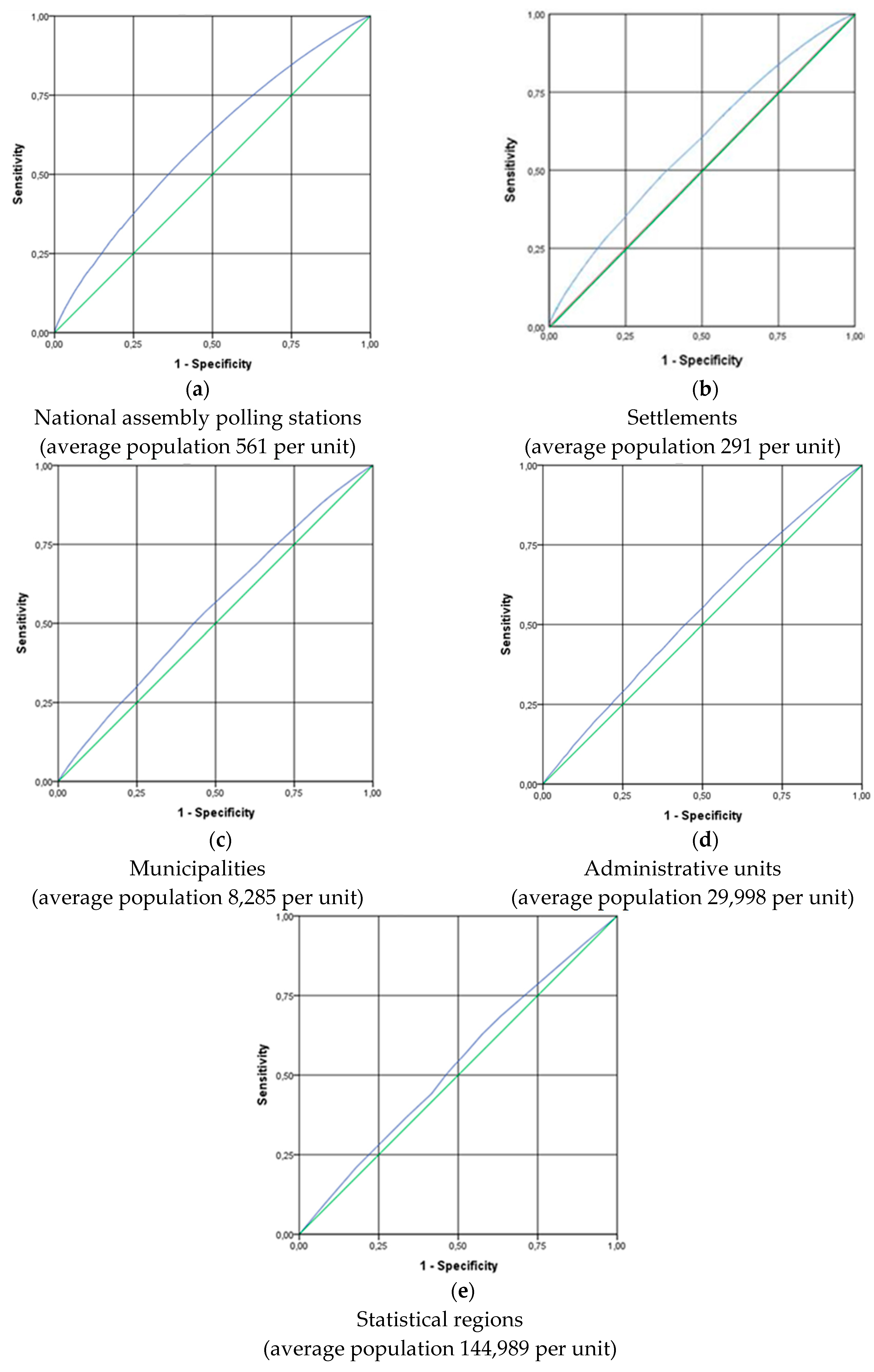
3.2. Assessment of the Ecological Fallacy
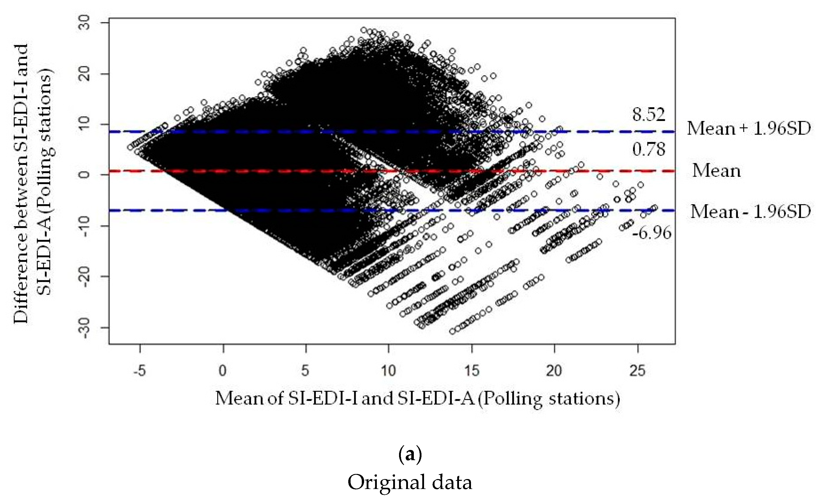
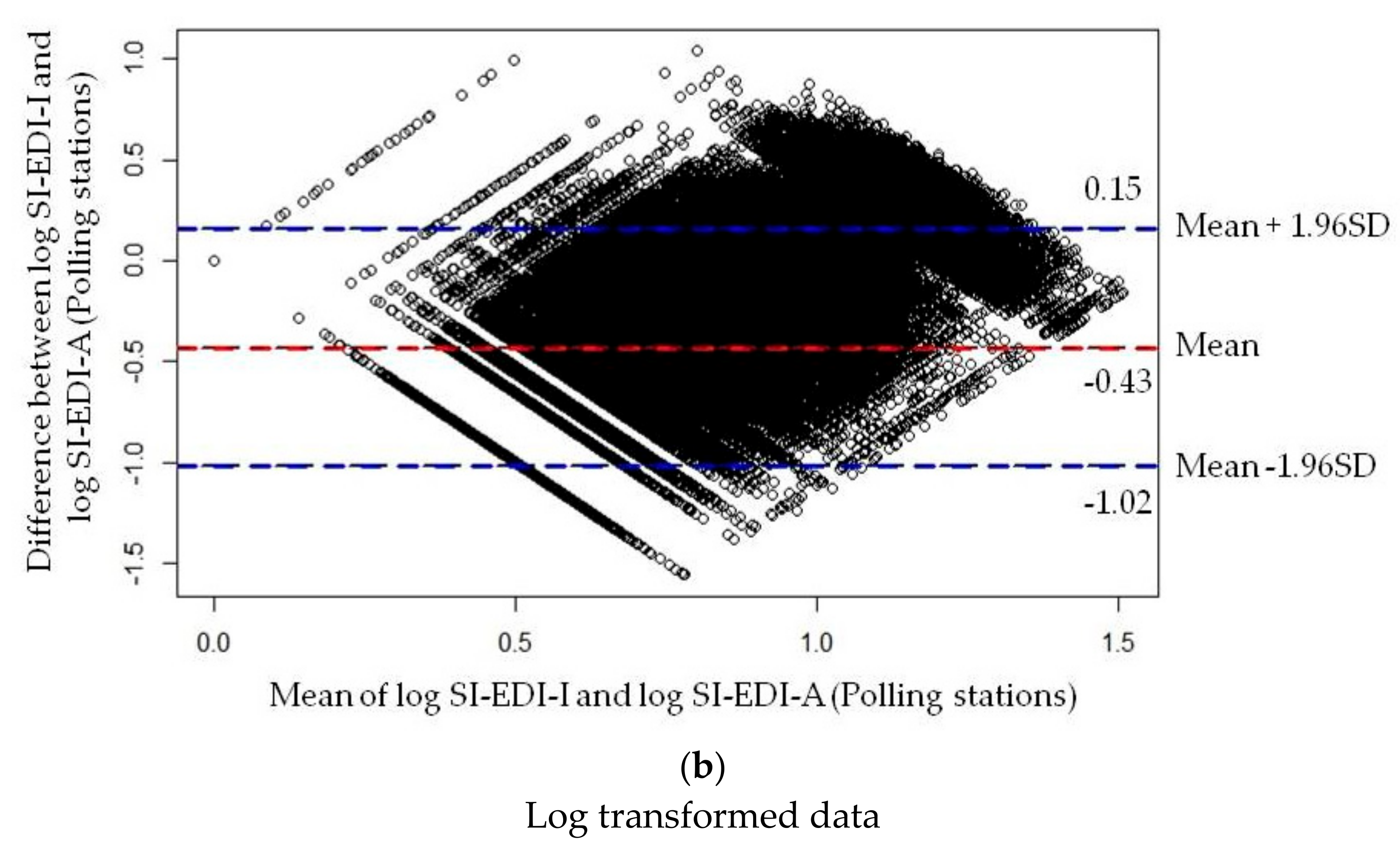
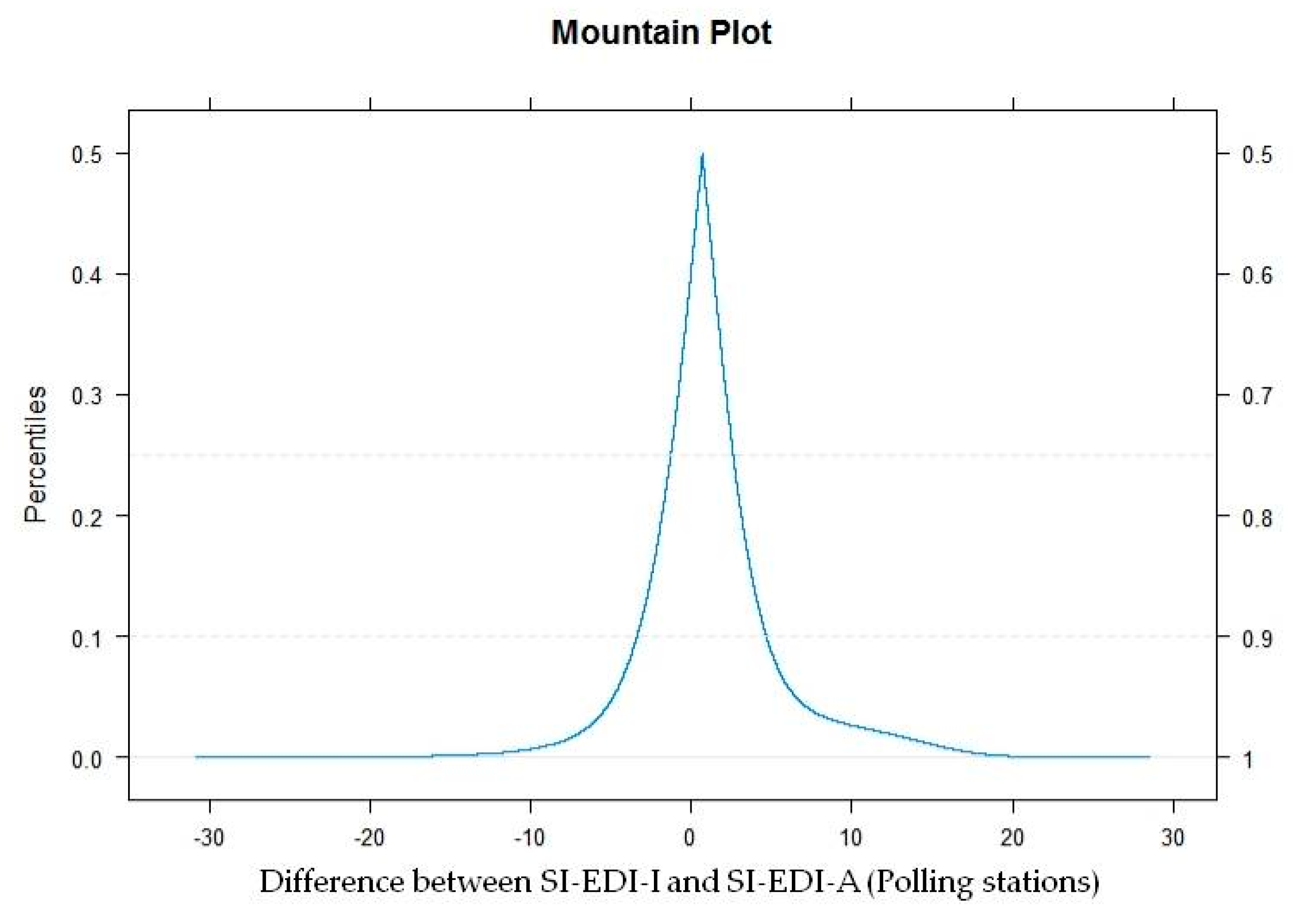
3.3. Agreement Analysis
3.4. Association of Socio-Economic Deprivation and Cancer Incidence
4. Discussion
5. Conclusions
Author Contributions
Funding
Acknowledgments
Conflicts of Interest
References
- Greenland, S. Ecologic versus individual-level sources of bias in ecologic estimates of contextual health effects. Int. J. Epidemiol. 2001, 30, 1343–1350. [Google Scholar] [CrossRef] [PubMed]
- Loney, T.; Nagelkerke, N.J. The individualistic fallacy, ecological studies and instrumental variables: A causal interpretation. Emerg. Themes Epidemiol. 2014, 11, 18. [Google Scholar] [CrossRef] [PubMed]
- Schwartz, S. The fallacy of the ecological fallacy: The potential misuse of a concept and the consequences. Am. J. Public Health 1994, 84, 819–824. [Google Scholar] [CrossRef] [PubMed]
- Eržen, I.; Gajšek, P.; Hlastan Ribič, C.; Kukec, A.; Poljšak, B.; Zaletel Kragelj, L. Zdravje in Okolje: Izbrana Poglavja, 1st ed.; Medicinska Fakulteta: Maribor, Slovenija, 2010; pp. 23–29. [Google Scholar]
- Connelly, R.; Playford, C.J.; Gayle, V.; Dibben, C. The role of administrative data in the big data revolution in social science research. Soc. Sci. Res. 2016, 59, 1–12. [Google Scholar] [CrossRef] [PubMed]
- Marra, C.A.; Lynd, L.D.; Harvard, S.S.; Grubisic, M. Agreement between aggregate and individual-level measures of income and education: A comparison across three patient groups. BMC Health Serv. Res. 2011, 11, 69. [Google Scholar] [CrossRef]
- Pampalon, P.; Hamel, D.; Gamache, P. A comparison of individual and area-based socio-economic data for monitoring social inequalities in health. Health Rep. 2009, 20, 85–94. [Google Scholar]
- Davey Smith, G.; Hart, C.; Watt, G.; Hole, D.; Hawthorne, V. Individual social class, area-based deprivation, cardiovascular disease risk factors, and mortality: The Renfrew and Paisley study. J. Epidemiol. Community Health 1998, 52, 399–405. [Google Scholar] [CrossRef]
- Geronimus, A.T.; Bound, J. Use of census-based aggregate variables to proxy for socioeconomic group: Evidence from national samples. Am. J. Epidemiol. 1998, 148, 475–486. [Google Scholar] [CrossRef]
- Greenwald, H.P.; Polissar, N.L.; Borgatta, E.F.; McCorkle, R. Detecting survival effects of socioeconomic status: Problems in the use of aggregate measures. J. Clin. Epidemiol. 1994, 47, 903–909. [Google Scholar] [CrossRef]
- Krieger, N. Overcoming the absence of socioeconomic data in medical records: Validation and application of a census-based methodology. Am. J. Public Health 1992, 82, 703–710. [Google Scholar] [CrossRef]
- Krieger, N.; Gordon, D. Re: «Use of census-based aggregate variables to proxy for socioeconomic group: Evidence from national samples». Am. J. Epidemiol. 1999, 150, 892–896. [Google Scholar] [CrossRef] [PubMed]
- Wilkins, R.; Tjepkema, M.; Mustard, C.; Choinière, R. The Canadian census mortality follow-up study, 1991 through 2001. Health Rep. 2008, 19, 24–43. [Google Scholar]
- Subramanian, S.V.; Chen, J.T.; Rehkopf, D.H.; Waterman, P.D.; Krieger, N. Comparing individual- and area-based socioeconomic measures for the surveillance of health disparities: A multilevel analysis of Massachusetts births, 1989–1991. Am. J. Epidemiol. 2006, 164, 823–834. [Google Scholar] [CrossRef] [PubMed]
- Davey Smith, G.; Hart, C. Re: «Use of census-based aggregate variables to proxy for socioeconomic group: Evidence from national samples». Am. J. Epidemiol. 1999, 150, 996–997. [Google Scholar] [CrossRef]
- Rehkopf, D.H.; Haughton, L.T.; Chen, J.T.; Waterman, P.D.; Subramanian, S.V.; Krieger, N. Monitoring socioeconomic disparities in death: Comparing individual-level education and area-based socioeconomic measures. Am. J. Public Health 2006, 96, 2135–2138. [Google Scholar] [CrossRef] [PubMed]
- Malešič, K. Metodologija Merjanja Blaginje Občin v Sloveniji na Osnovi Sestavljenih Kazalnikov; Magistrsko Delo, Ekonomska Fakulteta, Univerza v Ljubljani: Ljubljana, Slovenia, 2016; p. 9. [Google Scholar]
- Launoy, G.; Launay, L.; Dejardin, O.; Bryère, J.; Guillaume, G. European Deprivation Index: Designed to tackle socioeconomic inequalities in cancer in Europe: Guy Launoy. Eur. J. Public Health 2018, 28 (Suppl. 4), 214. [Google Scholar] [CrossRef]
- Guillaume, E.; Pornet, C.; Dejardin, O.; Launay, L.; Lillini, R.; Vercelli, M.; Marí-Dell’Olmo, M.; Fernández Fontelo, A.; Borrell, C.; Ribeiro, A.I.; et al. Development of a cross-cultural deprivation index in five European countries. J. Epidemiol. Community Health 2016, 70, 493–499. [Google Scholar] [CrossRef]
- Ribeiro, A.I.; Mayer, A.; Miranda, A.; Pina, M.F. The Portuguese version of the European Deprivation Index: An instrument to study health inequalities. Acta Med. Port 2017, 30, 17–25. [Google Scholar] [CrossRef]
- Zadnik, V.; Launay, L.; Guillaume, E.; Lokar, K.; Žagar, T.; Primic-Žakelj, M.; Launoy, G. Slovenian version of the European Deprivation Index at municipality level/Slovenska različica evropskega kazalnika primanjkljaja na ravni občin. Slov. J. Public Health/Zdr. Varst. 2018, 57, 47–54. [Google Scholar] [CrossRef]
- Antunes, L.; Mendonca, D.; Bento, M.J.; Rachet, B. No inequalities in survival from colorectal cancer by education and socioeconomic deprivation—A population-based study in the North Region of Portugal, 2000-2002. BMC Cancer 2016, 16, 608. [Google Scholar] [CrossRef]
- Bryere, J.; Dejardin, O.; Launay, L.; Colonna, M.; Grosclaude, P.; Launoy, G. French Network of Cancer Registries (FRANCIM) Socioeconomic status and site-specific cancer incidence, a Bayesian approach in a French Cancer Registries Network study. Eur. J. Cancer Prev. 2018, 27, 391–398. [Google Scholar] [CrossRef] [PubMed]
- Marquant, F.; Goujon, S.; Faure, L.; Guissou, S.; Orsi, L.; Hemon, D.; Lacour, B.; Clavel, J. Risk of childhood cancer and socio-economic disparities: Results of the French nationwide study Geocap 2002–2010. Paediatr. Perinat. Epidemiol. 2016, 30, 612–622. [Google Scholar] [CrossRef] [PubMed]
- Guillaume, E.; Launay, L.; Dejardin, O.; Bouvier, V.; Guittet, L.; Dean, P.; Notari, A.; De Mil, R.; Launoy, G. Could mobile mammography reduce social and geographic inequalities in breast cancer screening participation? Prev. Med. 2017, 100, 84–88. [Google Scholar] [CrossRef] [PubMed]
- Moriceau, G.; Bourmaud, A.; Tinquaut, F.; Oriol, M.; Jacquin, J.P.; Fournel, P.; Magné, N.; Chauvin, F. Social inequalities and cancer: Can the European deprivation index predict patients’ difficulties in health care access?: A pilot study. Oncotarget 2016, 7, 1055–1065. [Google Scholar] [CrossRef] [PubMed]
- Petit, M.; Bryere, J.; Maravic, M.; Pallaro, F.; Marcelli, C. Hip fracture incidence and social deprivation: Results from a French ecological study. Osteoporos. Int. 2017, 28, 2045–2051. [Google Scholar] [CrossRef] [PubMed]
- Albouy-Llaty, M.; Limousi, F.; Carles, C.; Dupuis, A.; Rabouan, S.; Migeot, V. Association between Exposure to Endocrine Disruptors in Drinking Water and Preterm Birth, Taking Neighborhood Deprivation into Account: A Historic Cohort Study. Int. J. Environ. Res. Public Health 2016, 13, 796. [Google Scholar] [CrossRef] [PubMed]
- Eurostat. EU-SILC: Description of Target Variables: Cross-Sectional and Longitudinal. 2011 Operation; European Commission, Eurostat: Brussels, Belgium, 2011. [Google Scholar]
- Dolenc, D. Registrski popis prebivalstva v letu 2011—Nov izziv slovenske državne statistike [Register based census 2011—A new challenge for the Slovenian national statistics]. In Merjenje Blaginje in Napredka Družbe: Izzivi pri Uporabi in Razumevanju Družbe [Measuring the Well-Being and the Progress of Society: Challenges in Using and Understanding the Data]; Noč Razinger, M., Panič, B., Zobec, I., Eds.; Statistical Office of the Republic of Slovenia, Statistical Society of Slovenia: Radenci, Slovenia, 2010; pp. 140–141. [Google Scholar]
- Cancer in Slovenia 2015; Institute of Oncology Ljubljana, Epidemiology and Cancer Registry, Cancer Registry of Republic of Slovenia: Ljubljana, Slovenia, 2018.
- Townsend, P. Deprivation. J. Soc. Policy 1987, 16, 125–146. [Google Scholar] [CrossRef]
- Pornet, C.; Delpierre, C.; Dejardin, O.; Grosclaude, P.; Launay, L.; Guittet, L.; Lang, T.; Launoy, G. Construction of an adaptable European transnational ecological deprivation index: The French version. J. Epidemiol. Community Health 2012, 6, 982–989. [Google Scholar] [CrossRef]
- Bryere, B.; Pornet, C.; Copin, N.; Launay, L.; Gusto, G.; Grosclaude, P.; Delpierre, C.; Lang, T.; Lantieri, O.; Dejardin, O.; et al. Assessment of the ecological bias of seven aggregate social deprivation indices. BMC Public Health 2016, 17, 86. [Google Scholar] [CrossRef]
- Bland, J.M.; Altman, D.G. Statistical methods for assessing agreement between two methods of clinical measurement. Lancet 1986, 1, 307–310. [Google Scholar] [CrossRef]
- Bland, J.M.; Altman, D.G. Measuring agreement in method comparison studies. Stat. Methods Med. Res. 1999, 8, 135–160. [Google Scholar] [CrossRef] [PubMed]
- Montenij, L.J.; Buhre, W.F.; Jansen, J.R.; Kruitwagen, C.L.; deWaal, E.E. Methodology of method comparison studies evaluating the validity of cardiac output monitors: A stepwise approach and checklist. Br. J. Anaesth. 2016, 116, 750–758. [Google Scholar] [CrossRef] [PubMed]
- Giavarina, D. Understanding Bland Altman analysis. Biochem. Med. 2015, 25, 141–151. [Google Scholar] [CrossRef]
- Krouwer, J.S.; Monti, K.L. A simple, graphical method to evaluate laboratory assays. Eur. J. Clin. Chem. Clin. Biochem. 1995, 33, 525–527. [Google Scholar]
- Lin, L.-K. A concordance correlation coefficient to evaluate reproducibility. Biometrics 1989, 45, 255–268. [Google Scholar] [CrossRef]
- Coxe, S.; West, S.G.; Aiken, L.S. The analysis of count data: A gentle introduction to poisson regression and its alternatives. J. Personal. Assess. 2009, 91, 121–136. [Google Scholar] [CrossRef] [PubMed]
- Parodi, S.; Bottarelli, E. Poisson regression model in epidemiology—An introduction. Ann. Fac. Med. Vet. Di Parma 2006, 26, 25–44. [Google Scholar]
- Breslow, N.E.; Day, N.E. The Design and Analysis of Cohort Studies. In Statistical Methods in Cancer Research; International Agency for Research on Cancer: Lyon, France, 1987; Volume 2, p. 133. [Google Scholar]
- Pascutto, C.; Wakefield, J.C.; Best, N.G.; Richardson, S.; Bernardinelli, L.; Staines, A.; Elliott, P. Statistical issues in the analysis of disease mapping data. Stat. Med. 2000, 19, 2493–2519. [Google Scholar] [CrossRef]
- Spiegelhalter, D.J.; Thomas, A.; Best, N.; Lunn, D. Winbugs Version 1.4 Software and User Manual; MRC Biostatistics Unit, University of Cambridge: Cambridge, UK, 2003; Available online: https://www.mrc-bsu.cam.ac.uk/wp-content/uploads/manual14.pdf (accessed on 10 October 2018).
- Besag, J.; York, J.; Molli´e, A. Bayesian Image Restoration, with Two Applications in Spatial Statistics. Ann. Inst. Stat. Math. 1991, 43, 1–20. [Google Scholar] [CrossRef]
- Altman, D.G.; Bland, J.M. Measurement in medicine: The analysis of method comparison studies. Statistician 1983, 32, 307–317. [Google Scholar] [CrossRef]
- van Stralen, K.J.; Dekker, F.W.; Zoccali, C.; Jager, K.J. Measuring agreement, More Complicated than It Seems. Nephron Clin. Pr. 2012, 120, 162–167. [Google Scholar] [CrossRef] [PubMed]
- Bryere, J.; Dejardin, O.; Bouvier, V.; Colonna, M.; Guizard, A.-V.; Troussard, X.; Pornet, C.; Galateau-Salle, F.; Bara, S.; Launay, L.; et al. Socioeconomic environment and cancer incidence: A French population-based study in Normandy. BMC Cancer 2014, 14, 87. [Google Scholar] [CrossRef] [PubMed]
- Schuurman, N.; Bell, N.; Dunn, J.R.; Oliver, L. Deprivation indices, population health and geography: An evaluation of the spatial effectiveness of indices at multiple scales. J. Urban Health 2007, 84, 591–603. [Google Scholar] [CrossRef] [PubMed]
- Farmer, J.C.; Baird, A.G.; Iversen, L. Rural deprivation: Reflecting reality. Br. J. Gen. Pr. 2001, 51, 486–491. [Google Scholar]
- Lalloué, B.; Monnez, J.M.; Padilla, C.; Kihal, W.; Le Meur, N.; Zmirou-Navier, D.; Deguen, S. A statistical procedure to create a neighbourhood socioeconomic index for health inequalities analysis. Int. J. Equity Health 2013, 12, 21. [Google Scholar] [CrossRef] [PubMed]
- Diez-Roux, A.V. A glossary for multilevel analysis. J. Epidemiol. Community Health 2002, 56, 588–594. [Google Scholar] [CrossRef] [PubMed]
- The World Factbook 2016-17; Central Intelligence Agency: Washington, DC, USA, 2016. Available online: https://www.cia.gov/library/publications/the-world-factbook/index.html (accessed on 3 January 2019).


| Level | SI-EDI-I | SI-EDI-A | ||||
|---|---|---|---|---|---|---|
| Individual | Polling Station | Settlement | Municipality | Administrative Unit | Statistical Region | |
| Number of units | 1,739,865 | 3104 | 5972 | 210 | 58 | 12 |
| % of study population in Quintile 1 1 | 16.8% | 23.2% | 20.0% | 15.6% | 36.8% | 35.6% |
| % of study population in Quintile 2 (cut off) | 22.8% (20%: −2.12) | 22.4% (20%: −2.86) | 19.9% (20%: −2.05) | 21.5% (20%: −2.90) | 22.0% (20%: −3.50) | 14.9% (20%: −3.84) |
| % of study population in Quintile 3 (cut off) | 20.0% (40%: −1.08) | 22.6% (40%: −1.52) | 7.0% (40%: −0.98) | 43.2% (40%: −1.37) | 13.5% (40%: −1.23) | 15.2% (40%: −0.31) |
| % of study population in Quintile 4 (cut off) | 20.1% (60%: −0.29) | 19.5% (60%: −0.01) | 33.0% (60%: −0.68) | 13.2% (60%: 0.26) | 15.9% (60%: 0.67) | 25.0% (60%: 0.86) |
| % of study population in Quintile 5 (cut off) 2 | 20.3% (80%: 1.37) | 12.3% (80%: 2.32) | 20.0% (80%: 0.03) | 6.4% (80%: 2.41) | 11.8% (80%: 3.36) | 9.3% (80%: 3.85) |
| Spatial Units (SI-EDI-A Levels) | Individual Deprivation (SI-EDI-I) |
|---|---|
| SI-EDI-A for national assembly polling stations | 0.600 [0.598, 0.601] |
| SI-EDI-A for settlements | 0.585 [0.584; 0.586] |
| SI-EDI-A for municipalities | 0.547 [0.546; 0.549] |
| SI-EDI-A for administrative units | 0.538 [0.537; 0.539] |
| SI-EDI-A for statistical regions | 0.530 [0.529; 0.531] |
| Category/Index | SI-EDI-A for National Assembly Polling Stations | SI-EDI-A for Settlements | SI-EDI-A for Municipalities | SI-EDI-A for Administrative Units | SI-EDI-A for Statistical Regions |
|---|---|---|---|---|---|
| Quintile 1 | 13.0% | 13.5% | 14.1% | 11.2% | 8.5% |
| Quintile 2 | 16.6% | 17.9% | 19.3% | 23.4% | 23.0% |
| Quintile 3 | 19.2% | 7.2% | 20.3% | 20.1% | 18.4% |
| Quintile 4 | 22.3% | 33.7% | 17.2% | 21.2% | 13.3% |
| Quintile 5 | 29.0% | 27.7% | 29.2% | 24.1% | 36.8% |
| Category/Index | SI-EDI-A for National Assembly Polling Stations | SI-EDI-A for Settlements | SI-EDI-A for Municipalities | SI-EDI-A for Administrative Units | SI-EDI-A for Statistical Regions |
|---|---|---|---|---|---|
| Quintile 1 | 21.8% | 21.7% | 18.7% | 14.1% | 10.1% |
| Quintile 2 | 20.9% | 20.5% | 20.5% | 26.0% | 26.5% |
| Quintile 3 | 20.2% | 7.0% | 21.0% | 19.8% | 17.2% |
| Quintile 4 | 19.4% | 32.9% | 15.6% | 19.7% | 12.4% |
| Quintile 5 | 17.8% | 18.0% | 24.3% | 20.5% | 33.7% |
| Sites | Topography (ICD−10) | Total Number of Cancer Cases | Estimation of SI-EDI-I Coefficient 1 | 95% CI 3 | Estimation of SI-EDI-A 2 | 95% CI 3 |
|---|---|---|---|---|---|---|
| Head and neck | C00–C14, C30–C32 | 1278 | 0.071 | 0.060 to 0.082 | 0.021 | 0.001 to 0.021 |
| Oesophagus | C15 | 241 | 0.056 | 0.031 to 0.082 | 0.061 | 0.022 to 0.096 |
| Stomach | C16 | 1396 | 0.033 | 0.022 to 0.044 | 0.009 | −0.011 to 0.027 |
| Colon and rectum | C18–C20 | 4398 | 0.028 | 0.021 to 0.034 | −0.004 | −0.015 to 0.006 |
| Pancreas | C25 | 1030 | 0.038 | 0.026 to 0.051 | −0.002 | −0.025 to 0.021 |
| Lung and trachea | C33–C34 | 3647 | 0.038 | 0.031 to 0.045 | 0.019 | 0.007 to 0.031 |
| Skin, melanoma | C43 | 1471 | −0.054 | −0.076 to −0.032 | −0.021 | −0.042 to −0.800 |
| Breast | C50 | 3692 | −0.003 | −0.012 to 0.007 | −0.018 | −0.031 to −0.005 |
| Cervix | C53 | 377 | 0.022 | −0.005 to 0.049 | −0.001 | −0.036 to 0.033 |
| Uterus | C54 | 928 | 0.033 | 0.019 to 0.046 | −0.020 | −0.045 to 0.003 |
| Prostate | C61 | 4418 | −0.014 | −0.022 to −0.006 | −0.017 | −0.029 to −0.004 |
| Testis | C62 | 302 | −0.050 | −0.105 to 0.004 | 0.003 | −0.035 to 0.041 |
| Kidney | C64–C65 | 1057 | 0.006 | −0.010 to 0.023 | −0.011 | −0.034 to 0.011 |
| Bladder | C67 | 926 | 0.022 | 0.008 to 0.036 | 0.002 | −0.023 to 0.026 |
| Thyroid | C73 | 431 | −0.075 | −0.112 to −0.038 | −0.016 | −0.052 to 0.018 |
| Non−Hodgkin’s lymphomas | C82−C85 | 1035 | 0.012 | −0.002 to 0.027 | −0.015 | −0.038 to 0.007 |
| Leukaemias | C91−C95 | 704 | 0.013 | −0.004 to 0.031 | −0.012 | −0.040 to 0.015 |
© 2019 by the authors. Licensee MDPI, Basel, Switzerland. This article is an open access article distributed under the terms and conditions of the Creative Commons Attribution (CC BY) license (http://creativecommons.org/licenses/by/4.0/).
Share and Cite
Lokar, K.; Zagar, T.; Zadnik, V. Estimation of the Ecological Fallacy in the Geographical Analysis of the Association of Socio-Economic Deprivation and Cancer Incidence. Int. J. Environ. Res. Public Health 2019, 16, 296. https://doi.org/10.3390/ijerph16030296
Lokar K, Zagar T, Zadnik V. Estimation of the Ecological Fallacy in the Geographical Analysis of the Association of Socio-Economic Deprivation and Cancer Incidence. International Journal of Environmental Research and Public Health. 2019; 16(3):296. https://doi.org/10.3390/ijerph16030296
Chicago/Turabian StyleLokar, Katarina, Tina Zagar, and Vesna Zadnik. 2019. "Estimation of the Ecological Fallacy in the Geographical Analysis of the Association of Socio-Economic Deprivation and Cancer Incidence" International Journal of Environmental Research and Public Health 16, no. 3: 296. https://doi.org/10.3390/ijerph16030296
APA StyleLokar, K., Zagar, T., & Zadnik, V. (2019). Estimation of the Ecological Fallacy in the Geographical Analysis of the Association of Socio-Economic Deprivation and Cancer Incidence. International Journal of Environmental Research and Public Health, 16(3), 296. https://doi.org/10.3390/ijerph16030296