Distributional Regression Techniques in Socioeconomic Research on the Inequality of Health with an Application on the Relationship between Mental Health and Income


Abstract
1. Introduction
1.1. A Review of the Methodological Literature
1.2. A Review of the Literature on Income and Mental Health
1.3. Aims and Structure of the Paper
2. Materials and Methods
2.1. Data
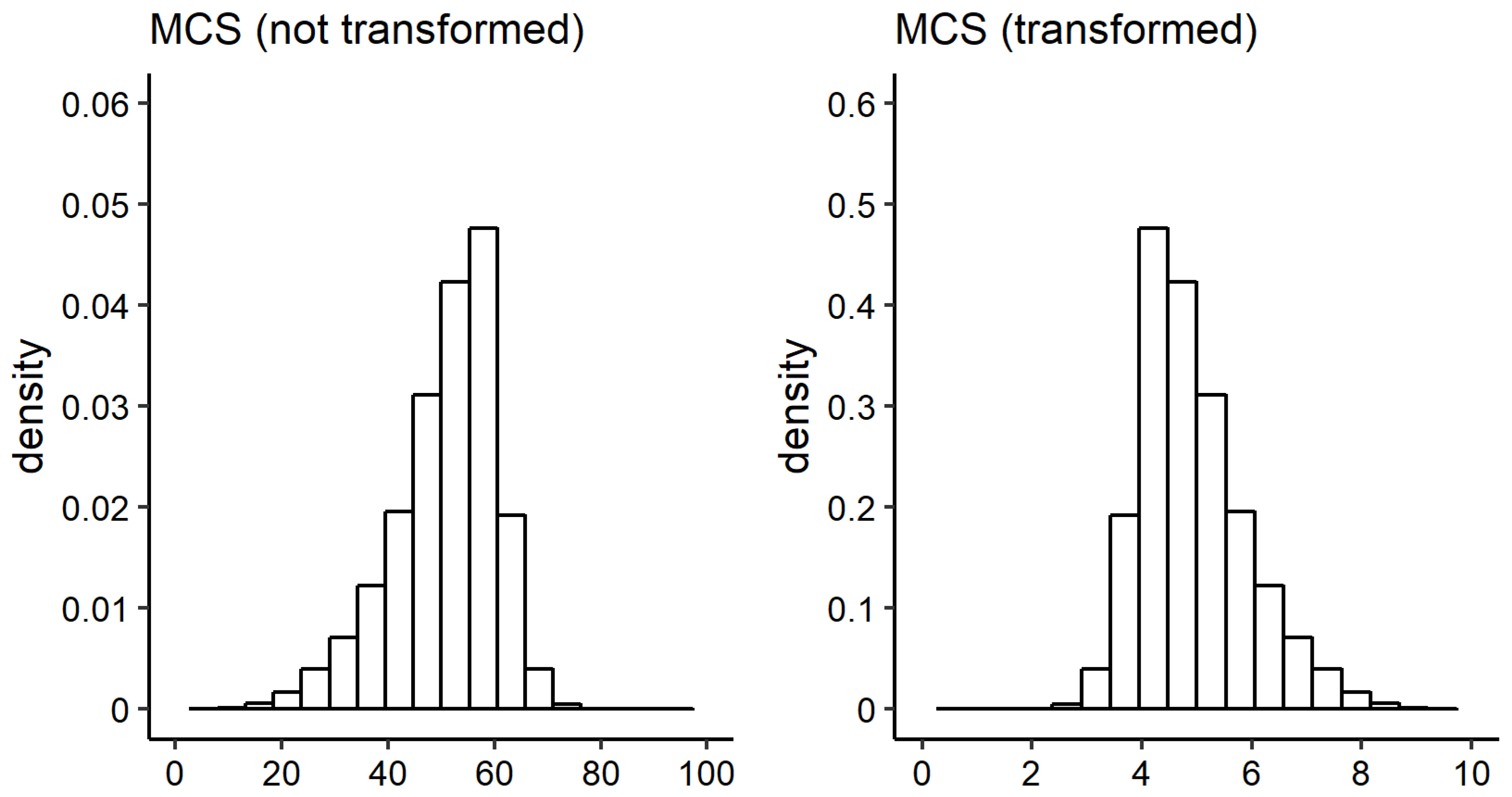
2.2. Conditional Health Assessment beyond the Mean
2.3. Considering the Conditional Distribution Set-Up
2.3.1. The Conditional Health Distribution
2.3.2. The Predictor Specification
2.3.3. The Link Function and Other Technical Aspects
3. Results
3.1. The Predictor
3.2. The Regression Coefficients
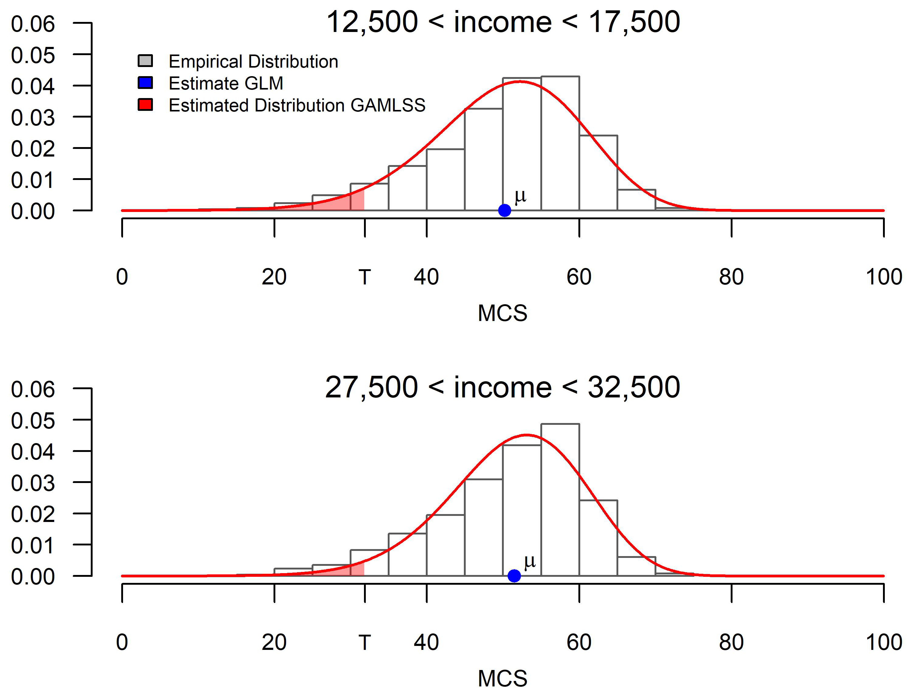
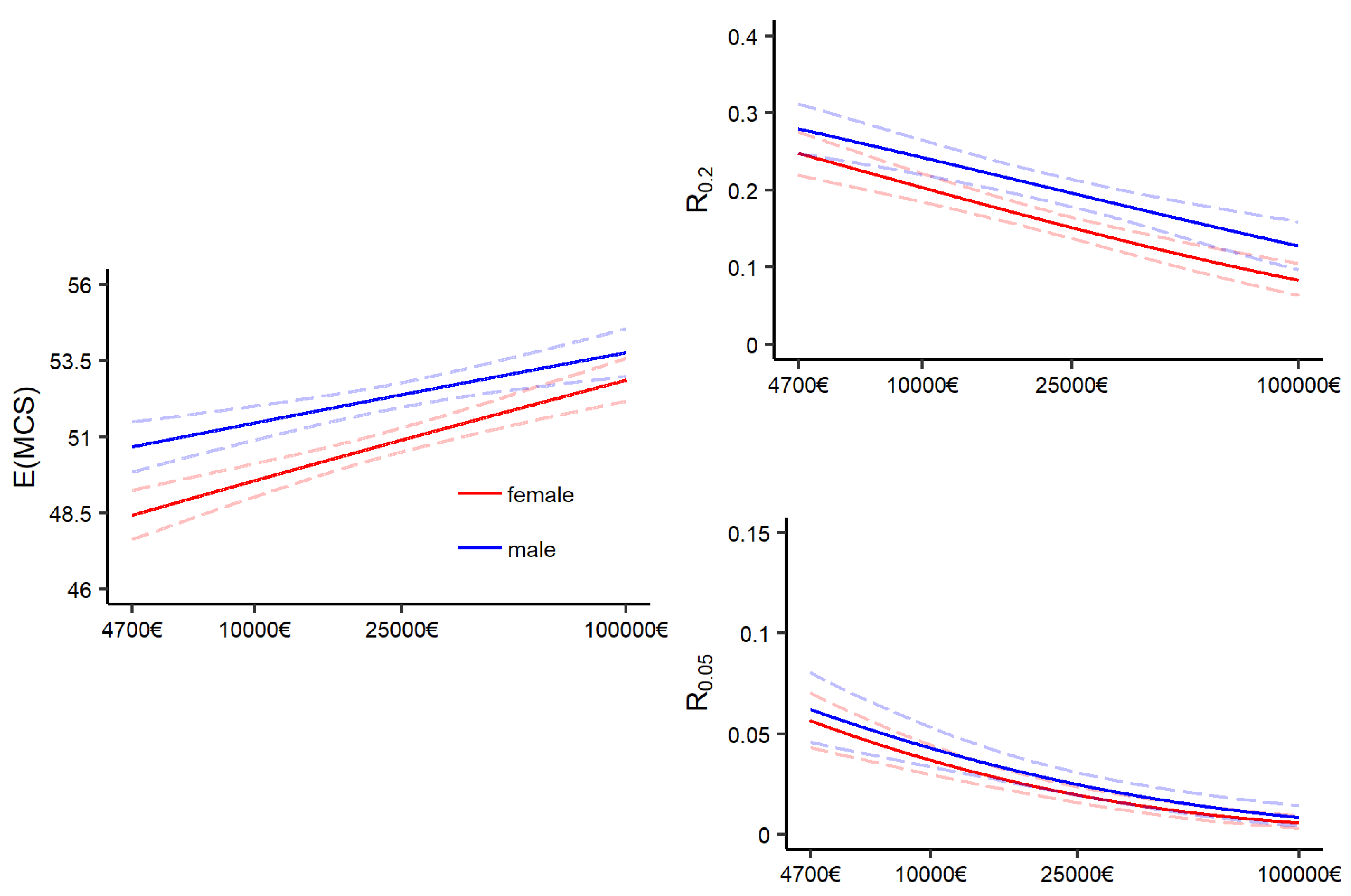
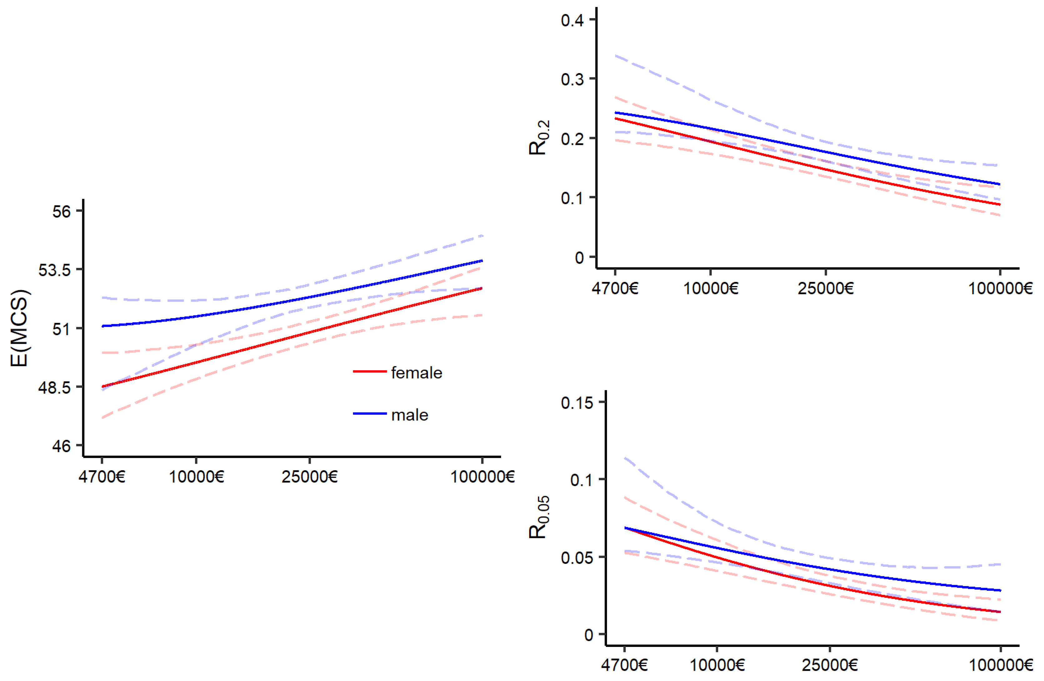
3.3. A Distributional Perspective on the Association between Mental Health and Income
3.3.1. Visualizing the Mental Health and Income Relationship
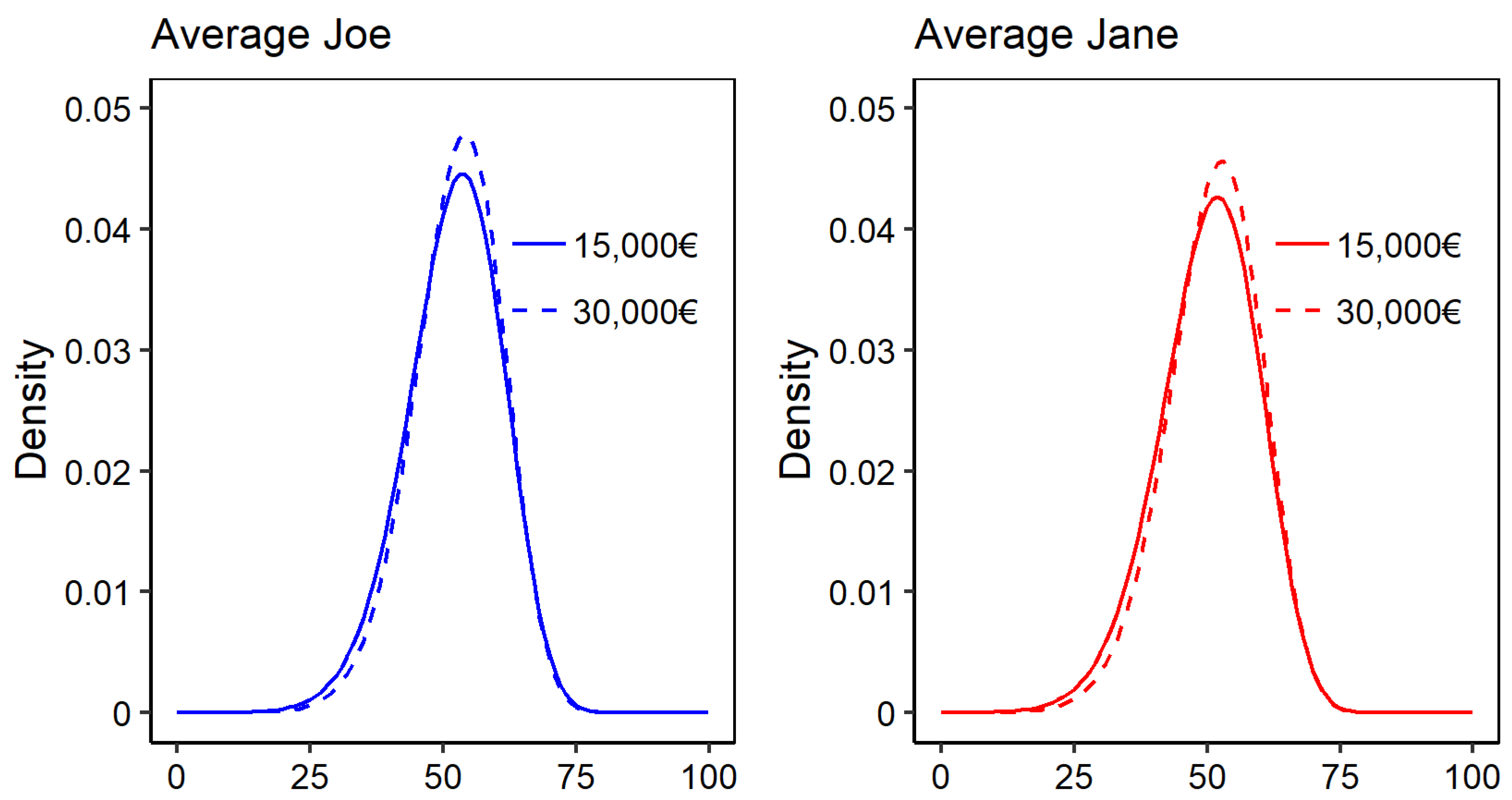
3.3.2. Contrasting Mental Health for Two Income Levels
4. Conclusions
Author Contributions
Funding
Conflicts of Interest
Abbreviations
| GLM | Generalised Linear Model |
| GAMLSS | Generalised Linear Models of Location, Scale & Shape |
| MCS | Mental Component Scale |
| PCS | Physical Component Scale |
Appendix A
Appendix A.1. Variables
Appendix A.2. Choosing a Distribution for the Conditional Health Distribution

| Distribution | gamlss Name | Page | ||||
| Box–Cox power exponential (BCPE) | BCPE | ident. | log | ident. | log | p. 291 |
| Box-Cox-Cole-Green (BCCG) | BCCG | ident. | log | ident. | - | p. 282 |
| Box–Cox-t (BCT) | BCT | ident. | log | ident. | log | p. 290 |
| Dagum (Da) | GB2 | log | log | log | = 1 | p. 294 |
| Gamma (Ga) | GA | log | log | - | - | p. 271 |
| Generalised Beta type 2 (GB2) | GB2 | log | log | log | log | p. 293 |
| Generalised Gamma (GG) | GG | log | log | ident. | - | p. 285 |
| Generalised Inverse Gaussian (GIG) | GIG | log | log | ident. | - | p. 287 |
| Log Normal (LOGNo) | LOGNO | ident. | log | - | - | p. 275 |
| Normal (No) | NO | ident. | log | - | - | p. 232 |
| Pearson-Type-VI (PtVI) | GB2 | log | = 1 | log | log | p. 293 |
| Singh-Maddala (SM) | GB2 | log | log | = 1 | log | p. 293 |
| Weibull (WEI3) | WEI3 | log | log | - | - | p. 280 |
| Model (Male) | AIC | BIC | GAIC () | TGDEV a |
|---|---|---|---|---|
| GB2 ( = 🗸, = 🗸, = 🗸, = ) | 20,734 † | 21,128 | 20,846 † | 5166 † |
| GB2 ( = 🗸, = 🗸, = –, = –) | 20,760 † | 20,971 † | 20,820 † | 5185 † |
| GB2 ( = 🗸, = 🗸, = 🗸, = –) | 20,763 † | 21,066 | 20,849 † | 5188 |
| Da ( = 🗸, = 🗸, = –) | 20,769 † | 20,973 † | 20,827 † | 5189 |
| BCT ( = 🗸, = 🗸, = 🗸, = –) | 20,777 † | 21,079 | 20,863 | 5184 † |
| Da ( = 🗸, = 🗸, = ) | 20,781 | 21,076 | 20,865 | 5189 |
| BCT ( = 🗸, = 🗸, = 🗸, = ) | 20,781 | 21,175 | 20,893 | 5187 |
| BCCG ( = 🗸, = 🗸, = ) | 20,783 | 21,078 | 20,867 | 5181 † |
| BCPE ( = 🗸, = 🗸, = 🗸, = –) | 20,784 | 21,086 | 20,870 | 5182 † |
| BCPE ( = 🗸, = 🗸, = 🗸, = ) | 20,786 | 21,179 | 20,898 | 5187 |
| BCT ( = 🗸, = 🗸, = –, = –) | 20,799 | 21,010 † | 20,859 † | 5197 |
| GG ( = 🗸, = 🗸, = –) | 20,809 | 21,012 † | 20,867 | 5190 |
| BCCG ( = 🗸, = 🗸, = –) | 20,810 | 21,013 † | 20,868 | 5192 |
| BCPE ( = 🗸, = 🗸, = –, = –) | 20,810 | 21,021 | 20,870 | 5195 |
| SM ( = 🗸, = 🗸, = –) | 20,848 | 21,052 | 20,906 | 5221 |
| SM ( = 🗸, = 🗸, = ) | 20,851 | 21,146 | 20,935 | 5220 |
| GIG ( = 🗸, = 🗸, = ) | 20,879 | 21,174 | 20,963 | 5233 |
| PtVI ( = 🗸, = 🗸, = ) | 20,903 | 21,198 | 20,987 | 5240 |
| GB2 ( = 🗸, = –, = –, = –) | 20,915 | 21,034 | 20,949 | 5242 |
| Da ( = 🗸, = –, = –) | 20,918 | 21,031 | 20,950 | 5244 |
| GIG ( = 🗸, = 🗸, = –) | 20,919 | 21,123 | 20,977 | 5248 |
| PtVI ( = 🗸, = 🗸, = –) | 20,929 | 21,133 | 20,987 | 5248 |
| BCT ( = 🗸, = –, = –, = –) | 20,938 | 21,058 | 20,972 | 5249 |
| BCPE ( = 🗸, = –, = –, = –) | 20,952 | 21,072 | 20,986 | 5250 |
| BCCG ( = 🗸, = –, = –) | 20,956 | 21,069 | 20,988 | 5246 |
| GG ( = 🗸, = –, = –) | 20,958 | 21,070 | 20,990 | 5246 |
| SM ( = 🗸, = –, = –) | 20,979 | 21,092 | 21,011 | 5267 |
| GIG ( = 🗸, = –, = –) | 21,006 | 21,119 | 21,038 | 5277 |
| LOGNo ( = 🗸, = ) | 21,020 | 21,216 | 21,076 | 5281 |
| PtVI ( = 🗸, = –, = –) | 21,028 | 21,141 | 21,060 | 5286 |
| LOGNo ( = 🗸, = –) | 21,146 | 21,251 | 21,176 | 5328 |
| Ga ( = 🗸, = ) | 21,267 | 21,464 | 21,323 | 5357 |
| Ga ( = 🗸, = –) | 21,381 | 21,486 | 21,411 | 5400 |
| No ( = 🗸, = ) | 22,040 | 22,237 | 22,096 | 5574 |
| No ( = 🗸, = –) | 22,148 | 22,253 | 22,178 | 5613 |
| WEI3 ( = 🗸, = ) | 23,305 | 23,501 | 23,361 | 5894 |
| WEI3 ( = 🗸, = –) | 23,341 | 23,447 | 23,371 | 5909 |
| Model (Male) | AIC | BIC | GAIC () | TGDEV a |
|---|---|---|---|---|
| BCPE ( = 🗸, = 🗸, = 🗸, = ) | 26,475 † | 26,878 | 26,587 † | 6617 |
| BCPE ( = 🗸, = 🗸, = 🗸, = –) | 26,487 † | 26,796 † | 26,573 † | 6603 † |
| GB2 ( = 🗸, = 🗸, = 🗸, = ) | 26,547 † | 26,950 | 26,659 | 6622 |
| BCCG ( = 🗸, = 🗸, = ) | 26,555 † | 26,857 | 26,639 † | 6612 † |
| BCT ( = 🗸, = 🗸, = 🗸, = –) | 26,557 † | 26,866 | 26,643 † | 6612 † |
| BCPE ( = 🗸, = 🗸, = –, = –) | 26,569 | 26,785 † | 26,629 † | 6623 |
| BCT ( = 🗸, = 🗸, = 🗸, = ) | 26,576 | 26,979 | 26,688 | 6612 † |
| GB2 ( = 🗸, = 🗸, = 🗸, = –) | 26,595 | 26,904 | 26,681 | 6613 † |
| GB2 ( = 🗸, = 🗸, = –, = –) | 26,605 | 26,821 † | 26,665 | 6624 |
| GG ( = 🗸, = 🗸, = –) | 26,615 | 26,824 † | 26,673 | 6627 |
| BCCG ( = 🗸, = 🗸, = –) | 26,621 | 26,829 † | 26,679 | 6629 |
| BCT ( = 🗸, = 🗸, = –, = –) | 26,623 | 26,839 | 26,683 | 6629 |
| GIG ( = 🗸, = 🗸, = ) | 26,626 | 26,928 | 26,710 | 6634 |
| PtVI ( = 🗸, = 🗸, = ) | 26,658 | 26,960 | 26,742 | 6639 |
| PtVI ( = 🗸, = 🗸, = –) | 26,659 | 26,867 | 26,717 | 6643 |
| GIG ( = 🗸, = 🗸, = –) | 26,668 | 26,877 | 26,726 | 6634 |
| LOGNo ( = 🗸, = ) | 26,723 | 26,924 | 26,779 | 6658 |
| Da ( = 🗸, = 🗸, = ) | 26,753 | 27,056 | 26,837 | 6643 |
| Da ( = 🗸, = 🗸, = –) | 26,764 | 26,973 | 26,822 | 6652 |
| BCPE ( = 🗸, = –, = –, = –) | 26,800 | 26,922 | 26,834 | 6650 |
| GG ( = 🗸, = –, = –) | 26,824 | 26,939 | 26,856 | 6651 |
| BCCG ( = 🗸, = –, = –) | 26,827 | 26,942 | 26,859 | 6653 |
| GIG ( = 🗸, = –, = –) | 26,828 | 26,943 | 26,860 | 6653 |
| BCT ( = 🗸, = –, = –, = –) | 26,829 | 26,952 | 26,863 | 6653 |
| GB2 ( = 🗸, = –, = –, = –) | 26,837 | 26,960 | 26,871 | 6651 |
| PtVI ( = 🗸, = –, = –) | 26,847 | 26,962 | 26,879 | 6659 |
| LOGNo ( = 🗸, = –) | 26,902 | 27,009 | 26,932 | 6676 |
| SM ( = 🗸, = 🗸, = ) | 26,903 | 27,205 | 26,987 | 6684 |
| Ga ( = 🗸, = ) | 26,921 | 27,123 | 26,977 | 6712 |
| SM ( = 🗸, = 🗸, = –) | 26,941 | 27,150 | 26,999 | 6694 |
| Da ( = 🗸, = –, = –) | 26,980 | 27,095 | 27,012 | 6674 |
| Ga ( = 🗸, = –) | 27,077 | 27,185 | 27,107 | 6727 |
| SM ( = 🗸, = –, = –) | 27,122 | 27,237 | 27,154 | 6711 |
| No ( = 🗸, = ) | 27,637 | 27,838 | 27,693 | 6902 |
| No ( = 🗸, = –) | 27,799 | 27,907 | 27,829 | 6920 |
| WEI3 ( = 🗸, = ) | 28,755 | 28,957 | 28,811 | 7190 |
| WEI3 ( = 🗸, = –) | 28,798 | 28,906 | 28,828 | 7198 |
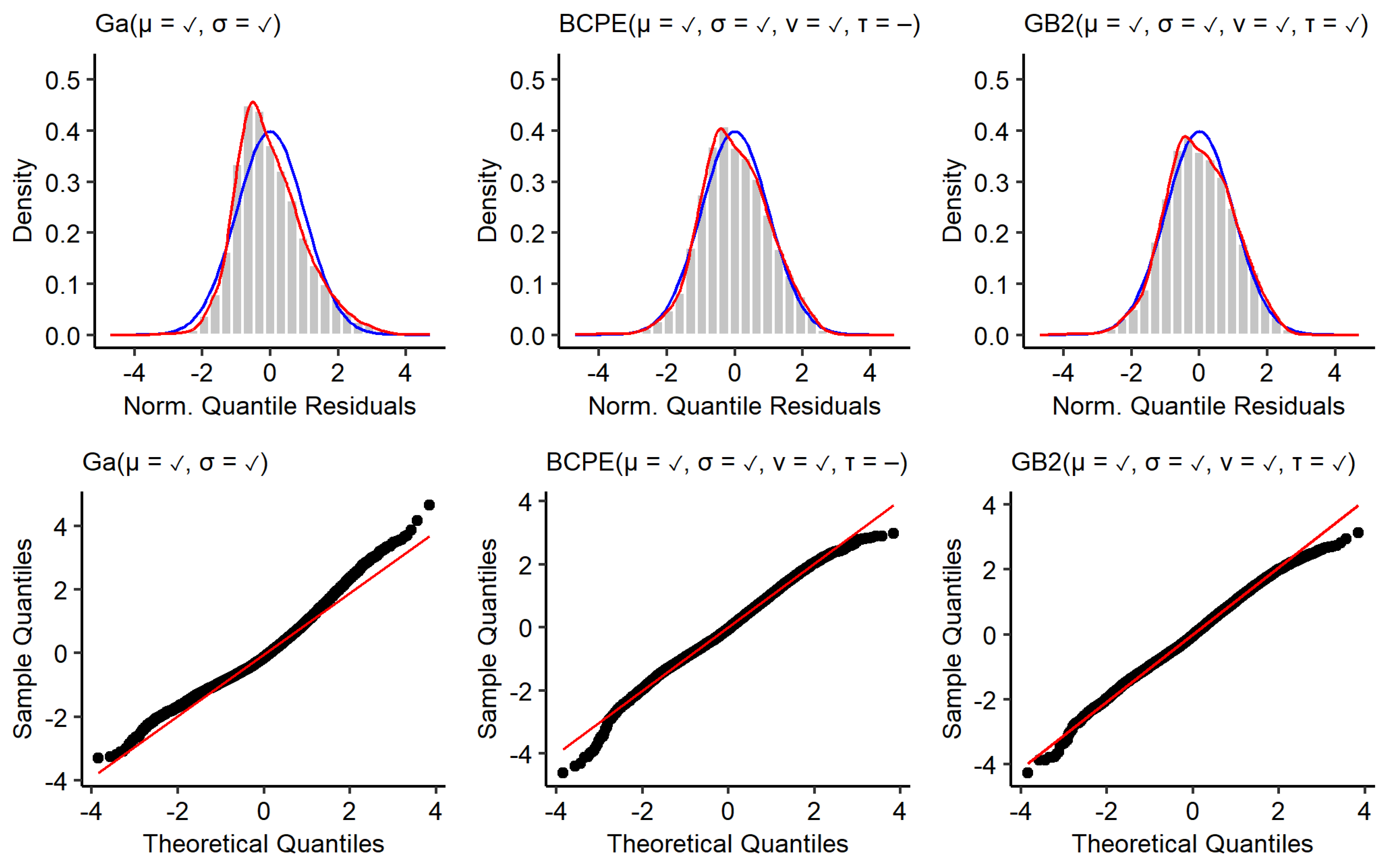
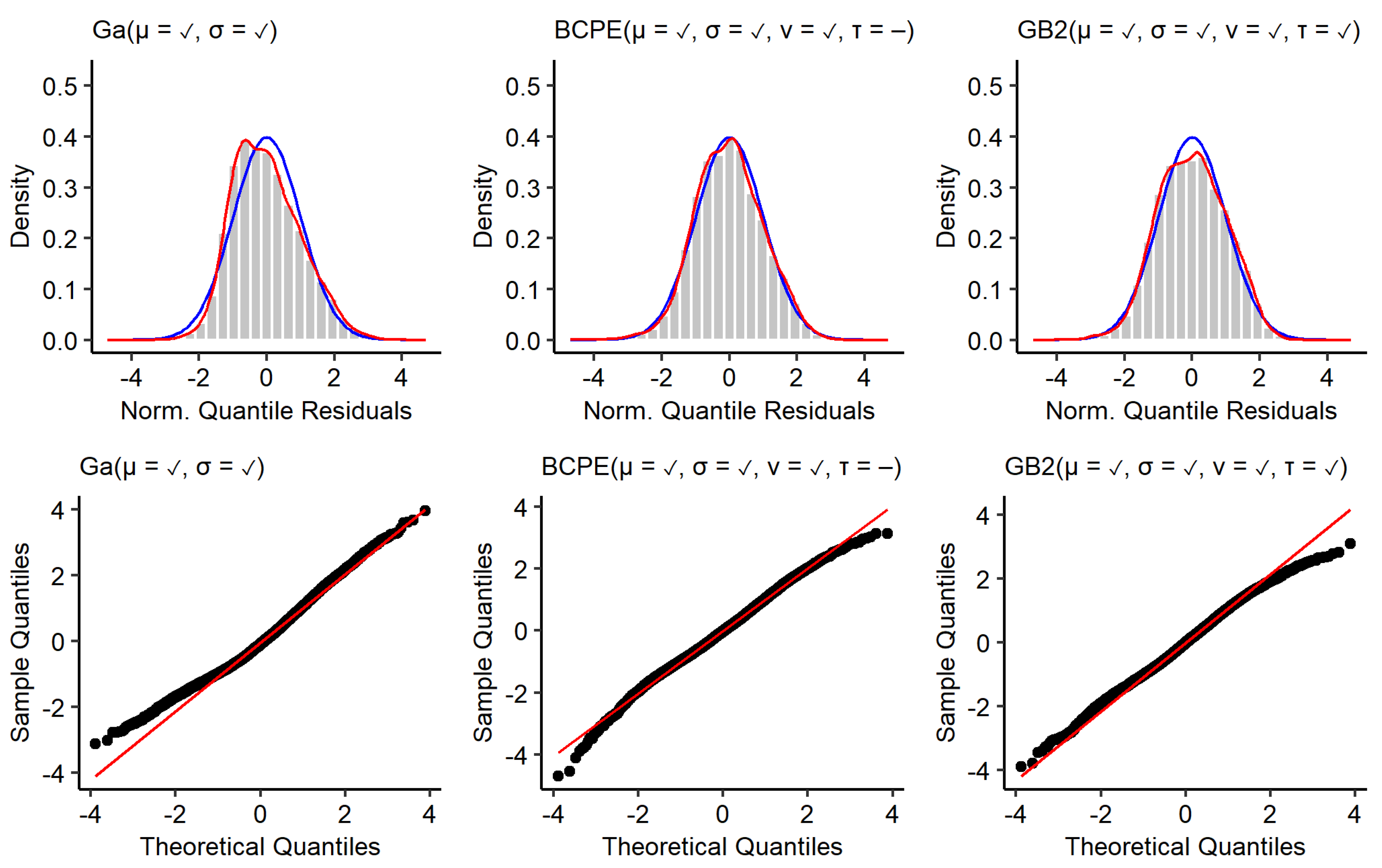
Appendix A.3. Residual Diagnostics


Appendix A.4. Distributional Measures of BCPE and GB2 Models


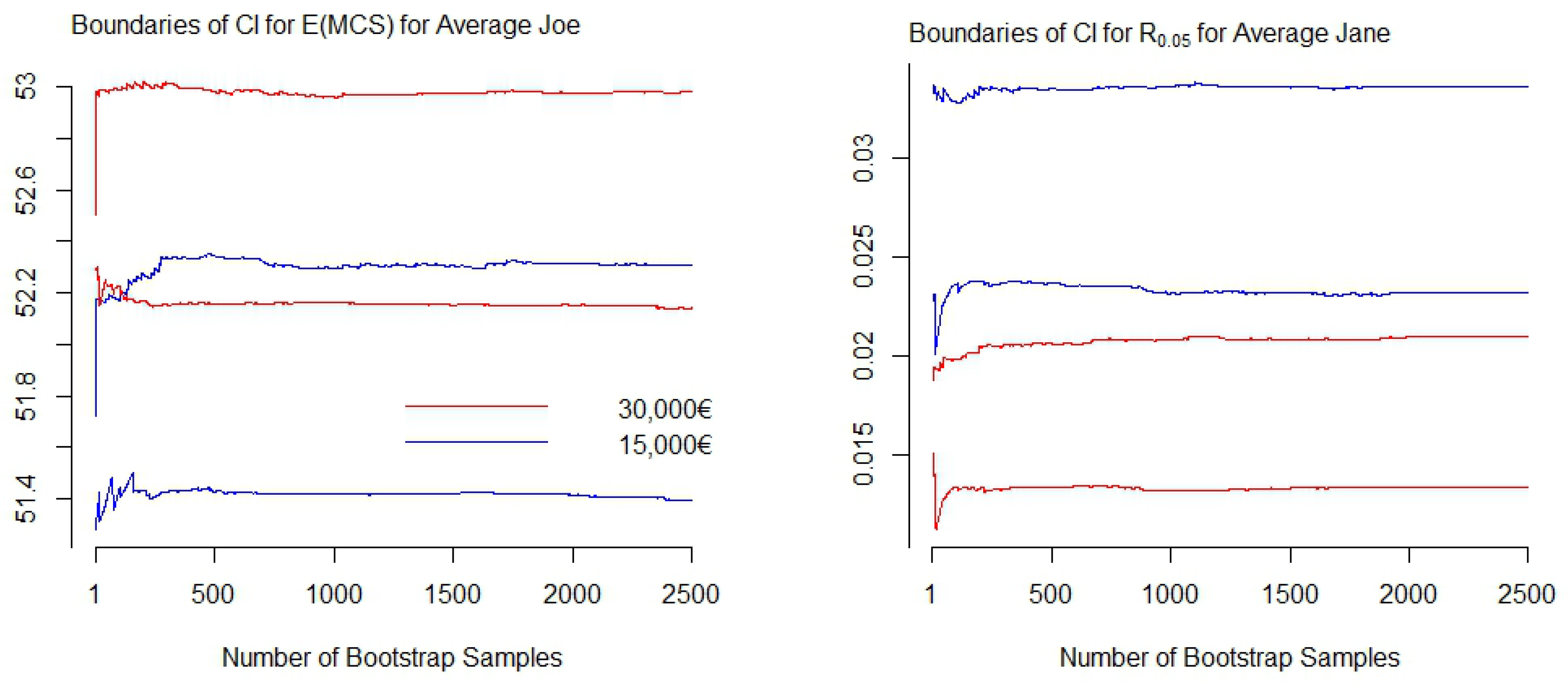
Appendix A.5. Bootstrap Confidence Intervals
- Create a bootstrap sample: Sample with replacement N observations from the training data.
- Estimate a GAMLSS model with the bootstrap sample.
- Calculate .
- Repeat steps one to three 2500 times to obtain estimates.
- Calculate the empirical 2.5% and 97.5% quantiles from the distribution of resulting from the 2500 bootstrap samples.

References
- Chetty, R.; Stepner, M.; Abraham, S.; Lin, S.; Scuderi, B.; Turner, N.; Bergeron, A.; Cutler, D. The association between income and life expectancy in the United States, 2001–2014. JAMA 2016, 315, 1750–1766. [Google Scholar] [CrossRef] [PubMed]
- Bird, Y.; Lemstra, M.; Rogers, M.; Moraros, J. The relationship between socioeconomic status/income and prevalence of diabetes and associated conditions: A cross-sectional population-based study in Saskatchewan, Canada. Int. J. Equity Health 2015, 14, 93. [Google Scholar] [CrossRef] [PubMed]
- Kaplan, M.S.; Huguet, N.; Feeny, D.H.; McFarland, B.H. Self-reported hypertension prevalence and income among older adults in Canada and the United States. Soc. Sci. Med. 2010, 70, 844–849. [Google Scholar] [CrossRef] [PubMed]
- Chandola, T.; Jenkinson, C. Validating self-rated health in different ethnic groups. Ethn. Health 2000, 5, 151–159. [Google Scholar] [CrossRef]
- DeSalvo, K.B.; Bloser, N.; Reynolds, K.; He, J.; Muntner, P. Mortality prediction with a single general self-rated health question: A meta-analysis. J. Gen. Intern. Med. 2006, 21, 267–275. [Google Scholar] [CrossRef]
- König, H.H.; Heider, D.; Lehnert, T.; Riedel-Heller, S.G.; Angermeyer, M.C.; Matschinger, H.; Vilagut, G.; Bruffaerts, R.; Haro, J.M.; de Girolamo, G.; et al. Health status of the advanced elderly in six European countries: Results from a representative survey using EQ-5D and SF-12. Health Qual. Life Outcomes 2010, 8, 143. [Google Scholar]
- Ware, J.E., Jr.; Kosinski, M.; Keller, S.D. A 12-Item Short-Form Health Survey: Construction of Scales and Preliminary Tests of Reliability and Validity. Med. Care 1996, 34, 220–233. [Google Scholar] [CrossRef]
- Ware, J.E.; Keller, S.D.; Kosinski, M. SF-36 Physical and Mental Health Summary Scales; Health Assessment Lab: Boston, MA, USA, 1994. [Google Scholar]
- Elgar, F.J.; McKinnon, B.; Torsheim, T.; Schnohr, C.W.; Mazur, J.; Cavallo, F.; Currie, C. Patterns of socioeconomic inequality in adolescent health differ according to the measure of socioeconomic position. Soc. Indic. Res. 2016, 127, 1169–1180. [Google Scholar] [CrossRef]
- Erreygers, G.; van Ourti, T. Measuring socioeconomic Inequality in Health, Health Care and Health Financing by Means of Rank-dependent Indices: A Recipe for Good Practice. J. Health Econ. 2011, 30, 685–694. [Google Scholar] [CrossRef]
- Fleurbaey, M.; Schokkaert, E. Unfair Inequalities in Health and Health Care. J. Health Econ. 2009, 28, 73–90. [Google Scholar] [CrossRef]
- Siegel, M.; Mielck, A.; Maier, W. Individual Income, Area Deprivation, and Health: Do Income-Related Health Inequalities Vary by Small Area Deprivation? Health Econ. 2015, 24, 1523–1530. [Google Scholar] [CrossRef] [PubMed]
- Jacobi, F.; Höfler, M.; Strehle, J.; Mack, S.; Gerschler, A.; Scholl, L.; Busch, M.; Maske, U.; Hapke, U.; Gaebel, W.; et al. Psychische Störungen in der Allgemeinbevölkerung. Der Nervenarzt 2014, 85, 77–87. [Google Scholar] [CrossRef] [PubMed]
- Sareen, J.; Afifi, T.O.; McMillan, K.A.; Asmundson, G.J. Relationship between household income and mental disorders: Findings from a population-based longitudinal study. Arch. Gen. Psychiatry 2011, 68, 419–427. [Google Scholar] [CrossRef] [PubMed]
- Kahneman, D.; Deaton, A. High income improves evaluation of life but not emotional well-being. Proc. Natl. Acad. Sci. USA 2010, 107, 16489–16493. [Google Scholar] [CrossRef]
- Kushlev, K.; Dunn, E.W.; Lucas, R.E. Higher income is associated with less daily sadness but not more daily happiness. Soc. Psychol. Personal. Sci. 2015, 6, 483–489. [Google Scholar] [CrossRef]
- Erreygers, G.; Kessels, R. socioeconomic Status and Health: A New Approach to the Measurement of Bivariate Inequality. Int. J. Environ. Res. Public Health 2017, 14, 673. [Google Scholar] [CrossRef]
- Koenker, R.; Bassett, G. Regression Quantiles. Econometrica 1978, 46, 33–50. [Google Scholar] [CrossRef]
- Sobotka, F.; Kneib, T. Geoadditive Expectile Regression. Comput. Stat. Data Anal. 2012, 56, 755–767. [Google Scholar] [CrossRef]
- Hothorn, T.; Kneib, T.; Bühlmann, P. Conditional Transformation Models. J. R. Stat. Soc. Ser. B (Stat. Methodol.) 2014, 76, 3–27. [Google Scholar] [CrossRef]
- Chernozhukov, V.; Fernandez-Val, I.; Melly, B. Inference on Counterfactual Distributions. Econometrica 2013, 81, 2205–2268. [Google Scholar] [CrossRef]
- Firpo, S.; Fortin, N.M.; Lemieux, T. Unconditional Quantile Regressions. Econometrica 2009, 77, 953–973. [Google Scholar] [CrossRef]
- Stasinopoulos, D.M.; Rigby, R.A. Generalized Additive Models for Location, Scale and Shape (GAMLSS) in R. J. Stat. Softw. 2007, 23, 1–46. [Google Scholar] [CrossRef]
- Klein, N.; Kneib, T.; Lang, S.; Sohn, A. Bayesian Structured Additive Distributional Regression with an Application to Regional Income Inequality in Germany. Ann. Appl. Stat. 2015, 9, 1024–1052. [Google Scholar] [CrossRef]
- Carrieri, V.; Jones, A.M. The Income-Health Relationship ‘Beyond the Mean’: New Evidence from Biomarkers. Health Econ. 2017, 26, 937–956. [Google Scholar] [CrossRef]
- Heckley, G.; Gerdtham, U.G.; Kjellsson, G. A General Method for Decomposing the Causes of socioeconomic Inequality in Health. J. Health Econ. 2016, 48, 89–106. [Google Scholar] [CrossRef]
- Silbersdorff, A.; Lynch, J.; Klasen, S.; Kneib, T. Reconsidering the Income-Health Relationship using Distributional Regression. Health Econ. 2018, 27, 1074–1088. [Google Scholar] [CrossRef]
- Kessels, R.; Erreygers, G. A Direct Regression Approach to Decomposing socioeconomic Inequality of Health. Health Econ. 2019, 28, 884–905. [Google Scholar] [CrossRef]
- Allen, J.; Balfour, R.; Bell, R.; Marmot, M. Social determinants of mental health. Int. Rev. Psychiatry 2014, 26, 392–407. [Google Scholar] [CrossRef]
- McManus, S.; Meltzer, H.; Brugha, T.; Bebbington, P.; Jenkins, R. Adult Psychiatric Morbidity in England, 2007: Results of a Household Survey; The NHS Information Centre for Health and Social Care: Leeds, UK, 2009. [Google Scholar]
- Fryers, T.; Melzer, D.; Jenkins, R. Social inequalities and the common mental disorders. Soc. Psychiatry Psychiatr. Epidemiol. 2003, 38, 229–237. [Google Scholar] [CrossRef]
- Lorant, V.; Deliège, D.; Eaton, W.; Robert, A.; Philippot, P.; Ansseau, M. socioeconomic inequalities in depression: A meta-analysis. Am. J. Epidemiol. 2003, 157, 98–112. [Google Scholar] [CrossRef]
- Müters, S.; Hoebel, J.; Lange, C. Diagnose Depression: Unterschiede bei Frauen und Männern. 2013. Available online: https://edoc.rki.de/bitstream/handle/176904/3112/2.pdf?sequence=1&isAllowed=y (accessed on 5 September 2019).
- Jacobi, F.; Höfler, M.; Siegert, J.; Mack, S.; Gerschler, A.; Scholl, L.; Busch, M.A.; Hapke, U.; Maske, U.; Seiffert, I.; et al. Twelve-month prevalence, comorbidity and correlates of mental disorders in Germany: The Mental Health Module of the German Health Interview and Examination Survey for Adults (DEGS1-MH). Int. J. Methods Psychiatr. Res. 2014, 23, 304–319. [Google Scholar] [CrossRef] [PubMed]
- Jacobi, F.; Höfler, M.; Strehle, J.; Mack, S.; Gerschler, A.; Scholl, L.; Busch, M.A.; Hapke, U.; Maske, U.; Seiffert, I.; et al. Twelve-months prevalence of mental disorders in the German Health Interview and Examination Survey for Adults–Mental Health Module (DEGS1-MH): A methodological addendum and correction. Int. J. Methods Psychiatr. Res. 2015, 24, 305–313. [Google Scholar] [CrossRef] [PubMed]
- Lampert, T.; Kroll, L.E.; Hapke, U.; Jacobi, F. Sozioökonomischer Status und psychische Gesundheit. In Public Health Forum; Elsevier: Berlin, Germany, 2014; Volume 22, pp. 6–8. [Google Scholar]
- Wirtz, M.A.; Morfeld, M.; Glaesmer, H.; Brähler, E. Normierung des SF-12 Version 2.0 zur Messung der gesundheitsbezogenen Lebensqualität in einer deutschen bevölkerungsrepräsentativen Stichprobe. Diagnostica 2018, 64, 215–226. [Google Scholar] [CrossRef]
- Wood, A.M.; Boyce, C.J.; Moore, S.C.; Brown, G.D. An evolutionary based social rank explanation of why low income predicts mental distress: A 17 year cohort study of 30,000 people. J. Affect. Disord. 2012, 136, 882–888. [Google Scholar] [CrossRef]
- McMillan, K.A.; Enns, M.W.; Asmundson, G.; Sareen, J. The association between income and distress, mental disorders, and suicidal ideation and attempts: Findings from the Collaborative Psychiatric Epidemiology Surveys. J. Clin. Psychiatry 2010, 71, 1168–1175. [Google Scholar] [CrossRef]
- Lee, S.U.; Oh, I.H.; Jeon, H.J.; Roh, S. Suicide rates across income levels: Retrospective cohort data on 1 million participants collected between 2003 and 2013 in South Korea. J. Epidemiol. 2017, 27, 258–264. [Google Scholar] [CrossRef]
- Sareen, J.; Jagdeo, A.; Cox, B.J.; Clara, I.; ten Have, M.; Belik, S.L.; de Graaf, R.; Stein, M.B. Perceived barriers to mental health service utilization in the United States, Ontario, and the Netherlands. Psychiatr. Serv. 2007, 58, 357–364. [Google Scholar] [CrossRef]
- Weich, S.; Lewis, G. Poverty, unemployment, and common mental disorders: Population based cohort study. BMJ 1998, 317, 115–119. [Google Scholar] [CrossRef]
- Lorant, V.; Croux, C.; Weich, S.; Deliège, D.; Mackenbach, J.; Ansseau, M. Depression and socioeconomic risk factors: 7-year longitudinal population study. Br. J. Psychiatry 2007, 190, 293–298. [Google Scholar] [CrossRef]
- Pickett, K.E.; Wilkinson, R.G. Income inequality and health: A causal review. Soc. Sci. Med. 2015, 128, 316–326. [Google Scholar] [CrossRef]
- Ribeiro, W.S.; Bauer, A.; Andrade, M.C.R.; York-Smith, M.; Pan, P.M.; Pingani, L.; Knapp, M.; Coutinho, E.S.F.; Evans-Lacko, S. Income inequality and mental illness-related morbidity and resilience: A systematic review and meta-analysis. Lancet Psychiatry 2017, 4, 554–562. [Google Scholar] [CrossRef]
- Daly, M.C.; Oswald, A.J.; Wilson, D.; Wu, S. Dark contrasts: The paradox of high rates of suicide in happy places. J. Econ. Behav. Organ. 2011, 80, 435–442. [Google Scholar] [CrossRef]
- Lucas, R.E.; Schimmack, U. Income and well-being: How big is the gap between the rich and the poor? J. Res. Personal. 2009, 43, 75–78. [Google Scholar] [CrossRef]
- Matz, S.C.; Gladstone, J.J.; Stillwell, D. Money buys happiness when spending fits our personality. Psychol. Sci. 2016, 27, 715–725. [Google Scholar] [CrossRef]
- Boyce, C.J.; Daly, M.; Hounkpatin, H.O.; Wood, A.M. Money may buy happiness, but often so little that it doesn’t matter. Psychol. Sci. 2017, 28, 544–546. [Google Scholar] [CrossRef] [PubMed]
- Westerhof, G.J.; Keyes, C.L. Mental illness and mental health: The two continua model across the lifespan. J. Adult Dev. 2010, 17, 110–119. [Google Scholar] [CrossRef] [PubMed]
- Boyce, C.J.; Brown, G.D.; Moore, S.C. Money and happiness: Rank of income, not income, affects life satisfaction. Psychol. Sci. 2010, 21, 471–475. [Google Scholar] [CrossRef]
- Yu, Z.; Chen, L. Income and well-being: Relative income and absolute income weaken negative emotion, but only relative income improves positive emotion. Front. Psychol. 2016, 7, 2012. [Google Scholar] [CrossRef]
- Sacks, D.W.; Stevenson, B.; Wolfers, J. The new stylized facts about income and subjective well-being. Emotion 2012, 12, 1181. [Google Scholar] [CrossRef]
- Silbersdorff, A. Analysing Inequalities in Germany; Springer: Berlin, Germany, 2017. [Google Scholar]
- Wagner, G.; Frick, J.; Schupp, J. The German socioeconomic Panel study (SOEP)—Scope, evolution and enhancements. Schmollers Jahrb. 2007, 127, 139–169. [Google Scholar]
- Glemser, A.; Huber, S.; Bohlender, A. SOEP 2014-TNS Report of SOEP Fieldwork in 2014; Technical Report, SOEP Survey Papers; SOEP: Berlin, Germany, 2015. [Google Scholar]
- Gruebner, O.; Rapp, M.A.; Adli, M.; Kluge, U.; Galea, S.; Heinz, A. Risiko für psychische Erkrankungen in Städten. Dtsch Arztebl Int. 2017, 114, 121–127. [Google Scholar] [CrossRef] [PubMed]
- Paul, K.I.; Moser, K. Unemployment impairs mental health: Meta-analyses. J. Vocat. Behav. 2009, 74, 264–282. [Google Scholar] [CrossRef]
- Paykel, E.; Abbott, R.; Jenkins, R.; Brugha, T.; Meltzer, H. Urban-rural mental health differences in Great Britain: Findings from the National Morbidity Survey. Psychol. Med. 2000, 30, 269–280. [Google Scholar] [CrossRef] [PubMed]
- Peen, J.; Dekker, J.; Schoevers, R.A.; Ten Have, M.; de Graaf, R.; Beekman, A.T. Is the prevalence of psychiatric disorders associated with urbanization? Soc. Psychiatry Psychiatr. Epidemiol. 2007, 42, 984–989. [Google Scholar] [CrossRef]
- Modini, M.; Joyce, S.; Mykletun, A.; Christensen, H.; Bryant, R.A.; Mitchell, P.B.; Harvey, S.B. The mental health benefits of employment: Results of a systematic meta-review. Australas. Psychiatry 2016, 24, 331–336. [Google Scholar] [CrossRef]
- Okulicz-Kozaryn, A. Unhappy metropolis (when American city is too big). Cities 2017, 61, 144–155. [Google Scholar] [CrossRef]
- Andersen, H.H.; Mühlbacher, A.; Nübling, M.; Schupp, J.; Wagner, G.G. Computation of standard values for physical and mental health scale scores using the SOEP version of SF-12v2. Schmollers Jahrb. 2007, 127, 171–182. [Google Scholar]
- Nübling, M.; Andersen, H.H.; Mühlbacher, A. Entwicklung eines Verfahrens zur Berechnung der körperlichen und psychischen Summenskalen auf Basis der SOEP-Version des SF 12 (Algorithmus); Technical Report, Data Documentation; German Institute for Economic Research: Berlin, Germany, 2006. [Google Scholar]
- Cunillera, O.; Tresserras, R.; Rajmil, L.; Vilagut, G.; Brugulat, P.; Herdman, M.; Mompart, A.; Medina, A.; Pardo, Y.; Alonso, J.; et al. Discriminative capacity of the EQ-5D, SF-6D, and SF-12 as measures of health status in population health survey. Qual. Life Res. 2010, 19, 853–864. [Google Scholar] [CrossRef]
- Maurischat, C.; Morfeld, M.; Kohlmann, T.; Bullinger, M. Lebensqualität: Nützlichkeit und Psychometrie des Health Survey SF-36/SF-12 in der Medizinischen Rehabilitation; Pabst Science Publ.: Lengerich, Germany, 2004. [Google Scholar]
- Fernando, S. Mental Health, Race and Culture; Macmillan International Higher Education: London, UK, 2010. [Google Scholar]
- Fernando, S. Mental Health Worldwide: Culture, Globalization and Development; Springer: Berlin/Heidelberg, Germany, 2014. [Google Scholar]
- Heinz, A. Psychische Gesundheit: Begriff und Konzepte; Kohlhammer Verlag: Stuttgart, Germany, 2016. [Google Scholar]
- Horwitz, A.V. An overview of sociological perspectives on the definitions, causes, and responses to mental health and illness. In A Handbook for the Study of Mental Health; Cambridge University Press: New York, NY, USA, 2010; pp. 6–19. [Google Scholar]
- Huber, M.; Knottnerus, J.A.; Green, L.; van der Horst, H.; Jadad, A.R.; Kromhout, D.; Leonard, B.; Lorig, K.; Loureiro, M.I.; van der Meer, J.W.; et al. How should we define health? BMJ 2011, 343, d4163. [Google Scholar] [CrossRef]
- Vaillant, G.E. Positive mental health: Is there a cross-cultural definition? World Psychiatry 2012, 11, 93–99. [Google Scholar] [CrossRef]
- WHO. Mental Health: A State of Well-Being. 2014. Available online: http://www.who.int/features/factfiles/mental_health/en/ (accessed on 5 September 2019).
- Fleishman, J.A.; Lawrence, W.F. Demographic Variation in SF-12 scores: True Differences or Differential Item Functioning? Med. Care 2003, 41, III75–III86. [Google Scholar] [CrossRef] [PubMed]
- Bourion-Bédès, S.; Schwan, R.; Laprevote, V.; Bédès, A.; Bonnet, J.L.; Baumann, C. Differential Item Functioning (DIF) of SF-12 and Q-LES-Q-SF Items among French Substance Users. Health Qual. Life Outcomes 2015, 13, 172. [Google Scholar] [CrossRef] [PubMed]
- Benjamini, Y. Simultaneous and selective inference: Current successes and future challenges. Biom. J. 2010, 52, 708–721. [Google Scholar] [CrossRef] [PubMed]
- R Core Team. R: A Language and Environment for Statistical Computing; R Foundation for Statistical Computing: Vienna, Austria, 2017. [Google Scholar]
- Silbersdorff, A. Assessing the Fit of Conditional Distributions Derived by Bayesian Structured Additive Distributional Regression; ZfS Working Paper, 03/2016; Georg-August-Universität: Göttingen, Germany, 2017. [Google Scholar]
- Box, G.E.P. Science and Statistics. J. Am. Stat. Assoc. 1976, 71, 791–799. [Google Scholar] [CrossRef]
- Rigby, R.A.; Stasinopoulos, D.M. Generalized additive models for location, scale and shape. J. R. Stat. Soc. Ser. C (Appl. Stat.) 2005, 54, 507–554. [Google Scholar] [CrossRef]
- Stasinopoulos, M.D.; Rigby, R.A.; Heller, G.Z.; Voudouris, V.; De Bastiani, F. Flexible Regression and Smoothing: Using GAMLSS in R; Chapman and Hall/CRC: Boca Raton, 2017. [Google Scholar]
- OECD. Classifying Educational Programmes: Manual for ISCED-97 Implementation in OECD Countries; Technical Report; Organisation for Economic Co-operation and Development: Paris, France, 1999. [Google Scholar]
- Bach, S.; Corneo, G.; Steiner, V. From Bottom to Top: The Entire Income Distribution in Germany, 1992–2003. Rev. Income Wealth 2009, 55, 303–330. [Google Scholar] [CrossRef]
- Box, G.E.P. Sampling and Bayes’ Inference in Scientific Modelling and Robustness. J. R. Stat. Soc. A 1980, 143, 383–430. [Google Scholar] [CrossRef]
- Fenske, N.; Fahrmeir, L.; Rzehak, P.; Höhle, M. Detection of Risk Factors for Obesity in Early Childhood with Quantile Regression Methods for Longitudinal Data; Department of Statistics, University of Munich: Munich, Germany, 2008. [Google Scholar]
- Thomas, G.; Pereira, A.I.d.A.; Lobos, C.M.V. Analysis of a longitudinal multilevel experiment using GAMLSSs. arXiv 2018, arXiv:1810.03085. [Google Scholar]
- Manwell, L.A.; Barbic, S.P.; Roberts, K.; Durisko, Z.; Lee, C.; Ware, E.; McKenzie, K. What is mental health? Evidence towards a new definition from a mixed methods multidisciplinary international survey. BMJ Open 2015, 5, e007079. [Google Scholar] [CrossRef]
- Klein, N.; Kneib, T.; Klasen, S.; Lang, S. Bayesian Structured Additive Distributional Regression for Multivariate Responses. J. R. Stat. Soc. Ser. C (Appl. Stat.) 2015, 64, 569–591. [Google Scholar] [CrossRef]
- Chalmers, A.F. Wege der Wissenschaft: Einführung in die Wissenschaftstheorie; Springer: Berlin/Heidelberg, Germany, 2007. [Google Scholar]
- Morfeld, M.; Bullinger, M. Der SF-36 Health Survey zur Erhebung und Dokumentation gesundheitsbezogener Lebensqualität. Phys. Med. Rehabil. Kurortmed. 2008, 18, 250–255. [Google Scholar] [CrossRef]
- Bährer-Kohler, S.; Carod-Artal, F.J. Global Mental Health: Prevention and Promotion; Springer: Cham, Switzerland, 2017. [Google Scholar]
- Diener, E.; Suh, E.M.; Lucas, R.E.; Smith, H.L. Subjective weil-being: Three decades of progress. Psychol. Bull. 1999, 125, 276–302. [Google Scholar] [CrossRef]
- Wittchen, H.U.; Hoyer, J. Klinische Psychologie & Psychotherapie; Springer: Berlin/Heidelberg, Germany; New York, NY, USA, 2011; Volume 2. [Google Scholar]
- Hagenaars, A.J.; De Vos, K.; Asghar Zaidi, M. Poverty Statistics in the Late 1980s: Research Based on Micro-Data; Office for Official Publications of the European: Luxembourg, 1994. [Google Scholar]
- Grabka, M.M. Codebook for the $PEQUIV File 1984–2016: CNEF Variables with Extended Income Information for the SOEP; Technical Report, Data Documentation; SOEP: Berlin, Germany, 2016. [Google Scholar]
- Jacobi, F.; Wittchen, H.U.; Hölting, C.; Höfler, M.; Pfister, H.; Müller, N.; Lieb, R. Prevalence, co-morbidity and correlates of mental disorders in the general population: Results from the German Health Interview and Examination Survey (GHS). Psychol. Med. 2004, 34, 597–611. [Google Scholar] [CrossRef] [PubMed]
- Rigby, R.A.; Stasinopoulos, M.D.; Heller, G.; De Bastiani, F. Distributions for Modelling Location, Scale and Shape: Using GAMLSS in R. 2017. Available online: http://www.gamlss.com (accessed on 5 September 2019).


| Male | Female | ||||||||
|---|---|---|---|---|---|---|---|---|---|
| const. | 1.771 *** | (0.045) | −1.003 *** | (0.172) | 1.944 *** | (0.043) | −0.994 *** | (0.158) | |
| MAR2 | 0.018 * | (0.008) | 0.115 *** | (0.028) | 0.031 *** | (0.006) | 0.075 *** | (0.022) | |
| MAR3 | 0.007 | (0.006) | 0.052 * | (0.025) | 0.021 *** | (0.006) | 0.042 . | (0.022) | |
| MAR4 | 0.043 ** | (0.014) | 0.036 | (0.048) | 0.025 ** | (0.009) | 0.028 | (0.03) | |
| GER | −0.019 ** | (0.007) | −0.028 | (0.027) | −0.032 *** | (0.006) | −0.035 | (0.025) | |
| UNEMPLOYED | −0.026 ** | (0.010) | −0.048 | (0.034) | −0.027 ** | (0.009) | −0.094 ** | (0.029) | |
| EDUC2 | −0.007 | (0.007) | −0.046 . | (0.027) | −0.020 *** | (0.006) | −0.038 . | (0.021) | |
| EDUC3 | −0.004 | (0.009) | −0.052 | (0.032) | −0.002 | (0.008) | −0.006 | (0.028) | |
| EDUC4 | −0.008 | (0.008) | −0.101 *** | (0.031) | −0.016 * | (0.007) | −0.056 * | (0.026) | |
| CITY | 0.014 *** | (0.004) | 0.012 | (0.016) | 0.005 | (0.004) | −0.013 | (0.015) | |
| EAST | 0.008 . | (0.005) | −0.036 . | (0.019) | 0.003 | (0.005) | 0.001 | (0.017) | |
| AGE | 0.003 *** | (0.001) | 0.005 | (0.003) | 0.001 | (0.001) | 0.001 | (0.003) | |
| AGESQ | 0.000 *** | (0.000) | 0.000 | (0.000) | 0.000 ** | (0.000) | 0.000 | (0.000) | |
| LOGINC | −0.021 *** | (0.004) | −0.083 *** | (0.017) | −0.029 *** | (0.004) | −0.070 *** | (0.015) | |
| 15,000€ | 30,000€ | Relative Difference | |||||
|---|---|---|---|---|---|---|---|
| male | 51.86 | [51.4 ; 52.31] | 52.56 | [52.14; 52.98] | 0.013 | [0.008 ; 0.02] | |
| 0.222 | [0.203 ; 0.241] | 0.187 | [0.168 ; 0.205] | 0.158 | [0.105 ; 0.216] | ||
| 0.034 | [0.027 ; 0.042] | 0.022 | [0.017 ; 0.028] | 0.358 | [0.256 ; 0.456] | ||
| female | 50.15 | [49.72 ; 50.6] | 51.16 | [50.74 ; 51.57] | 0.020 | [0.014 ; 0.026] | |
| 0.180 | [0.165 ; 0.195] | 0.141 | [0.127 ; 0.156] | 0.214 | [0.161 ; 0.265] | ||
| 0.028 | [0.023 ; 0.034] | 0.017 | [0.013 ; 0.021] | 0.401 | [0.311 ; 0.483] | ||
© 2019 by the authors. Licensee MDPI, Basel, Switzerland. This article is an open access article distributed under the terms and conditions of the Creative Commons Attribution (CC BY) license (http://creativecommons.org/licenses/by/4.0/).
Share and Cite
Silbersdorff, A.; Schneider, K.S. Distributional Regression Techniques in Socioeconomic Research on the Inequality of Health with an Application on the Relationship between Mental Health and Income. Int. J. Environ. Res. Public Health 2019, 16, 4009. https://doi.org/10.3390/ijerph16204009
Silbersdorff A, Schneider KS. Distributional Regression Techniques in Socioeconomic Research on the Inequality of Health with an Application on the Relationship between Mental Health and Income. International Journal of Environmental Research and Public Health. 2019; 16(20):4009. https://doi.org/10.3390/ijerph16204009
Chicago/Turabian StyleSilbersdorff, Alexander, and Kai Sebastian Schneider. 2019. "Distributional Regression Techniques in Socioeconomic Research on the Inequality of Health with an Application on the Relationship between Mental Health and Income" International Journal of Environmental Research and Public Health 16, no. 20: 4009. https://doi.org/10.3390/ijerph16204009
APA StyleSilbersdorff, A., & Schneider, K. S. (2019). Distributional Regression Techniques in Socioeconomic Research on the Inequality of Health with an Application on the Relationship between Mental Health and Income. International Journal of Environmental Research and Public Health, 16(20), 4009. https://doi.org/10.3390/ijerph16204009