An Inexact Optimization Model for Crop Area Under Multiple Uncertainties


Abstract
1. Introduction
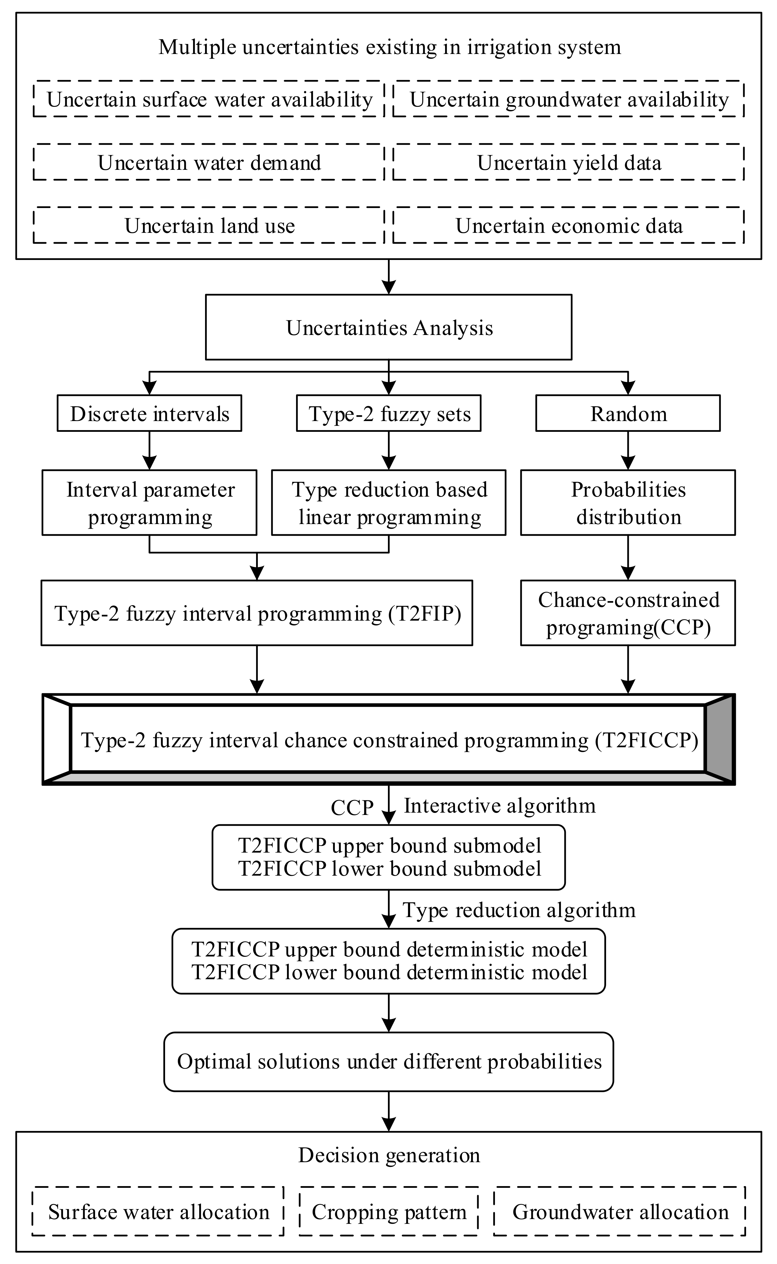
2. Model Formulation
2.1. Type-2 Fuzzy Interval Programming
2.2. The Chance Constrained Programming Model
2.3. Type-2 Fuzzy Interval Chance Constrained Programming
2.4. Solution Process
- Step 1: Establish the T2FICCP model.
- Step 2: Convert the chance constraint into the deterministic constraint with a feasible constraint set based on the CCP model.
- Step 3: Transform the model, which has converted the chance constraint into the deterministic constraint, into two submodels with T2FS based on the interactive algorithm.
- Step 4: Each submodel is converted into its deterministic counterpart by using a type reduction technique.
- Step 5: The submodel corresponding to is formulated and solved first based on the solution steps presented in Section 2.1.
- Step 6: Based on the solution of the first submodel, the submodel corresponding to is formulated and solved.
- Step 7: Based on the solutions of two submodels, the solution of the established T2FICCP model can be obtained, which is expressed as a set of intervals: and .
- Step 8: Repeat steps 3–7 corresponding to different levels.
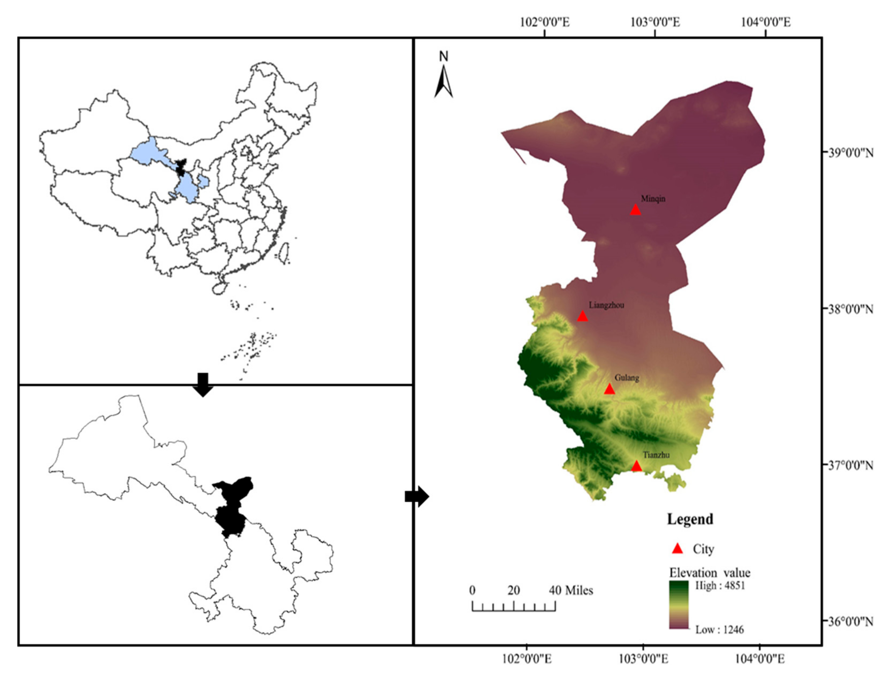
3. Case Study
Model Building
- : Price of crop i under the conventional irrigation mode (yuan/t) (Interval parameter);
- : Price of crop i under the water-saving irrigation mode (yuan/t) (Interval parameter);
- : Yield of crop i under the conventional irrigation mode (t/ha) (Interval parameter);
- : Yield of crop i under the water saving irrigation mode (t/ha) (Interval parameter);
- : The cost of crop i under the conventional irrigation mode (yuan/ha);
- : The cost of crop i under the water saving irrigation mode (yuan/ha);
- : Irrigation area of crop i (104 ha);
- : Minimized irrigation area of crop i (104 ha);
- : Maximized irrigation area of crop i (104 ha);
- TA: Total irrigation area of the study area (104 ha);
- : Irrigation quota of crop i under the conventional irrigation mode (m3/ha) (Interval number);
- : Irrigation quota of crop i under the water saving irrigation mode (m3/ha) (Interval number);
- IC: Irrigation water use efficiency of the study area;
- SW: Water demand of the secondary industry (104 m3);
- TW: Water demand of the tertiary industry (104 m3);
- DW: Domestic water consumption (104 m3);
- EW: Ecological water consumption (104 m3);
- : Groundwater exploration (104 m3) (Type-2 fuzzy interval parameter);
- SFW: Maximized surface water supply (104 m3) (Random parameter);
- : The ET of the ith crop under the conventional irrigation mode (m3/ha) (Interval parameter);
- : The ET of the ith crop under the water saving irrigation mode (m3/ha) (Interval parameter);
- TET: The control indicator of the total water consumption (m3);
- FDP: Food demand per capita (t/p);
- TPR: Population of the study area (104 p).
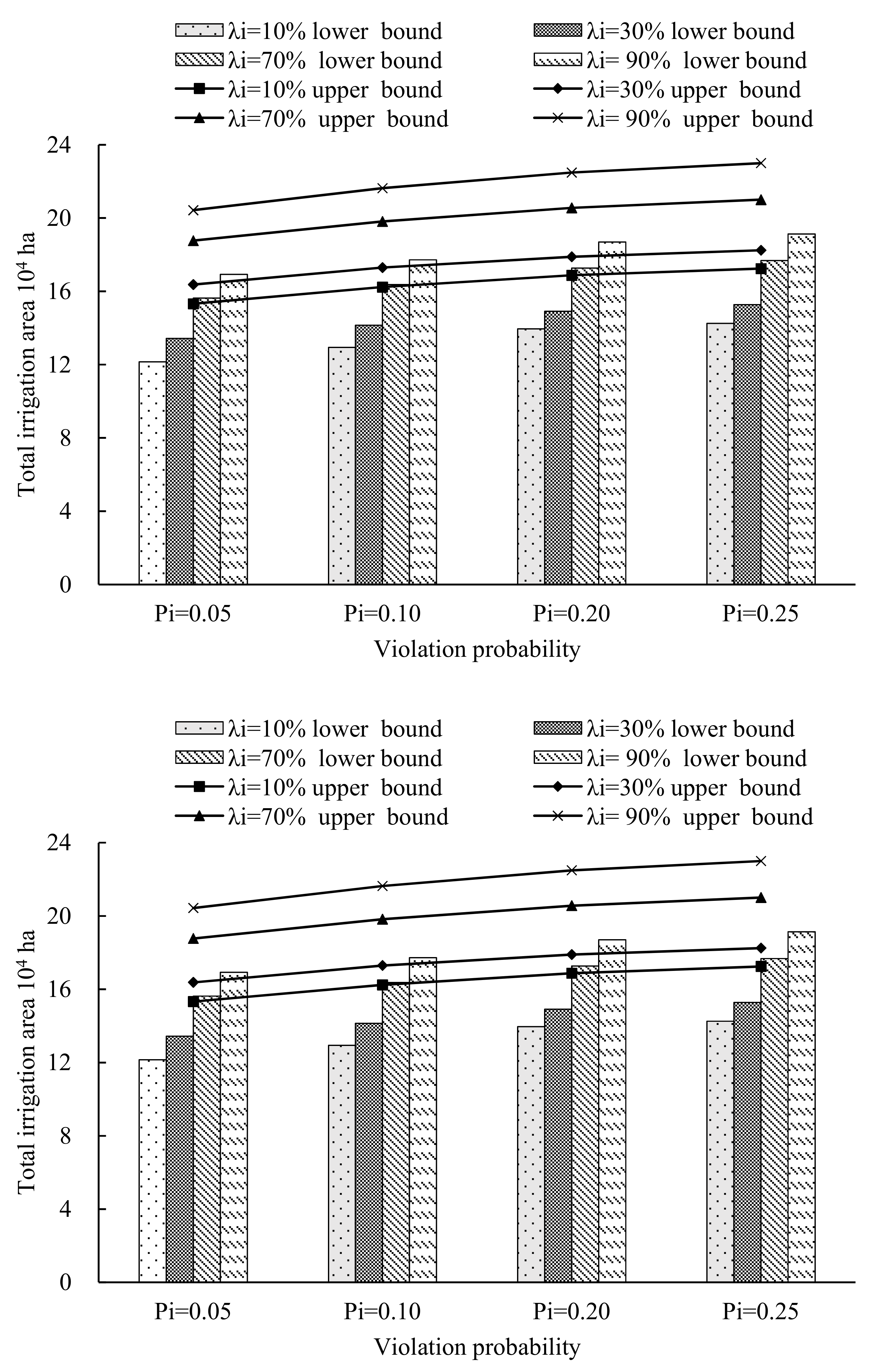
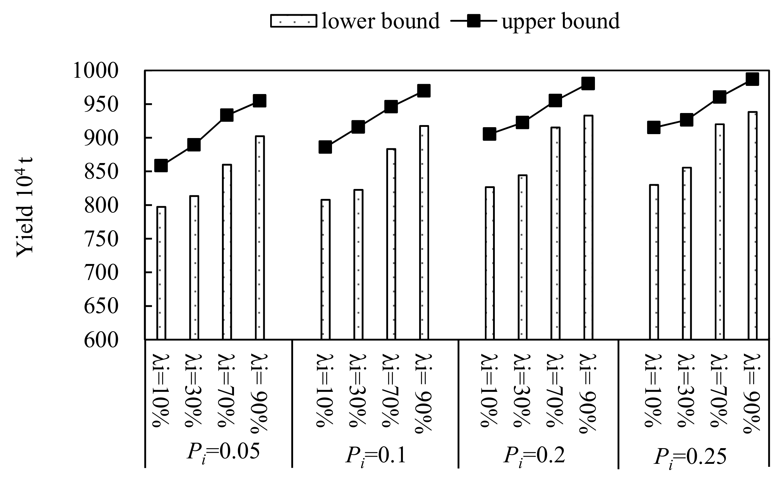
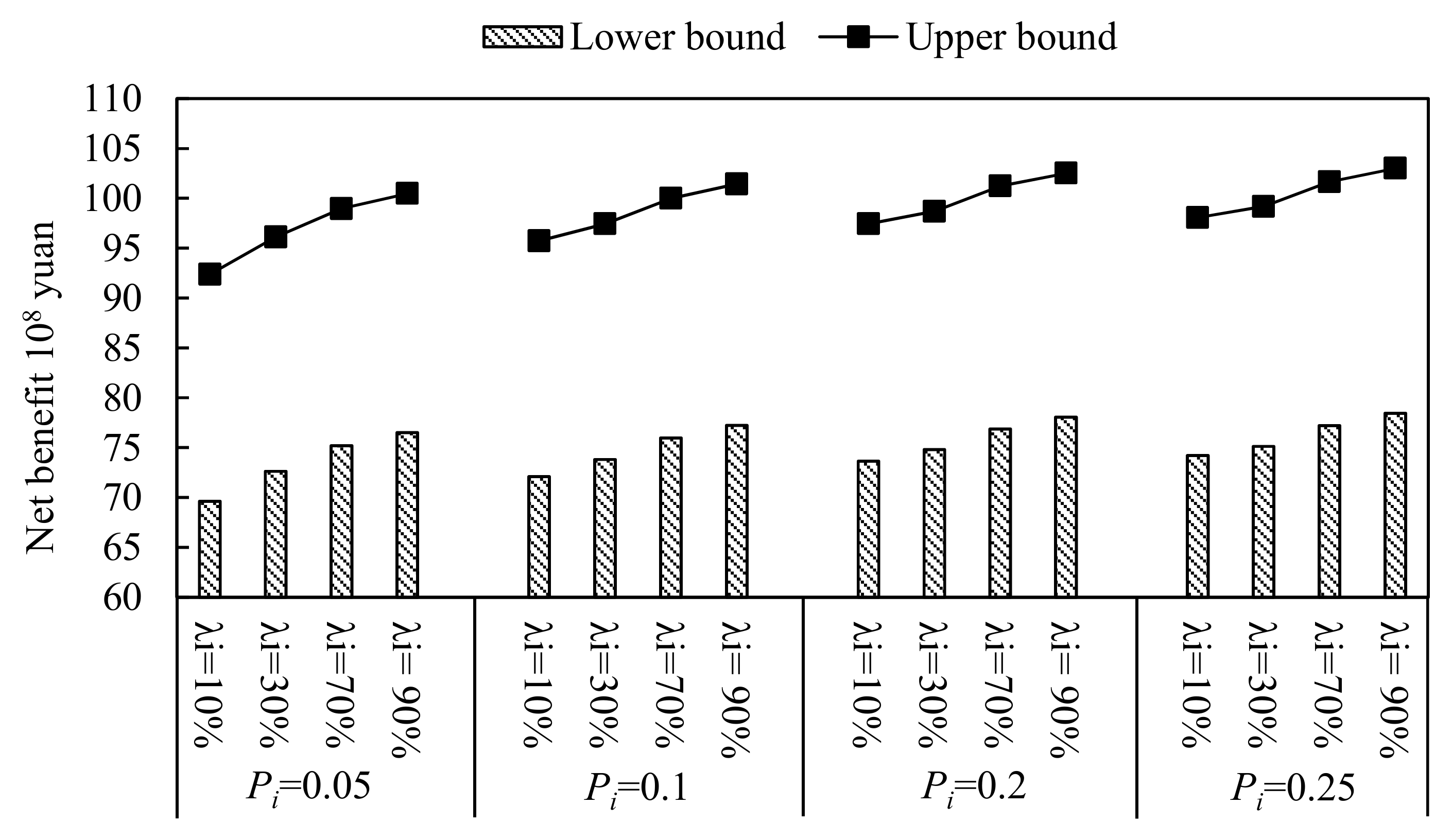
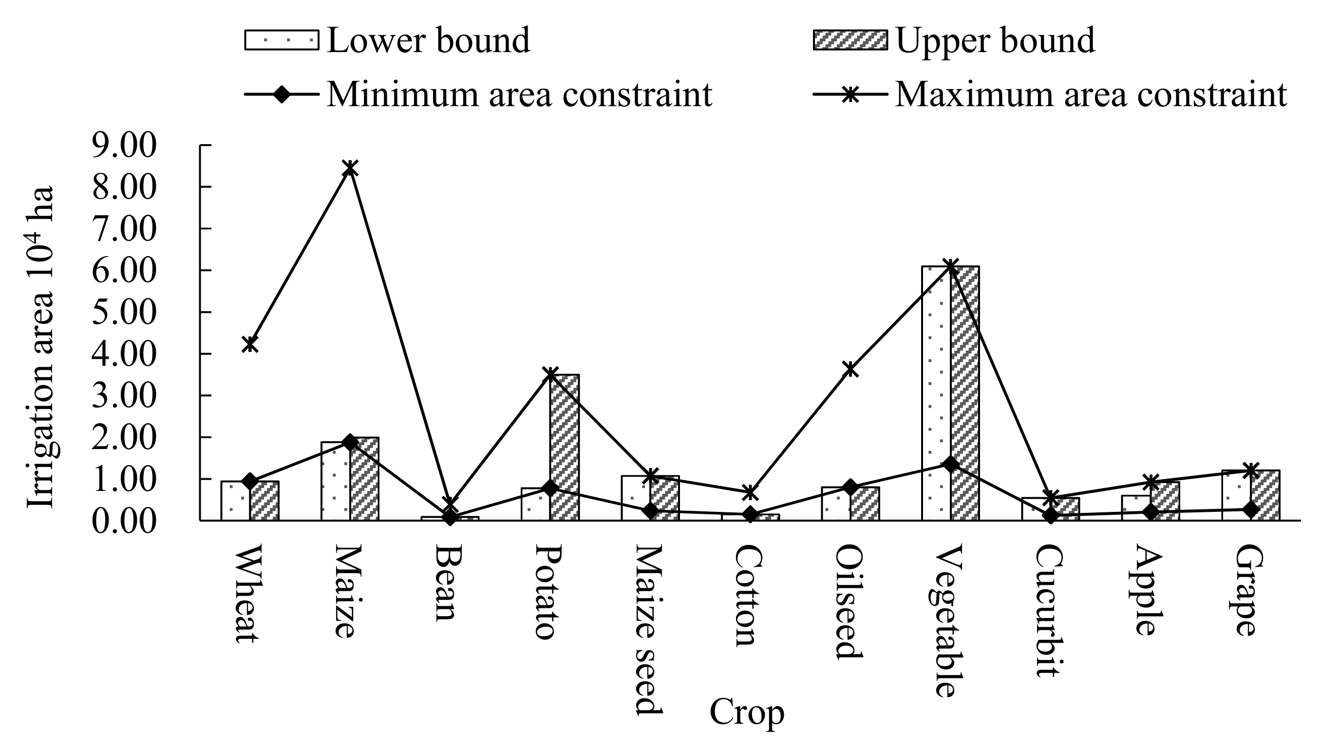
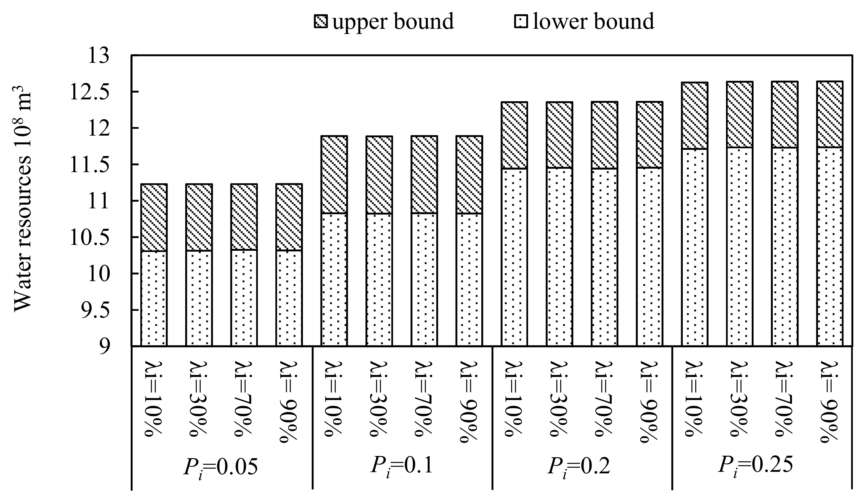
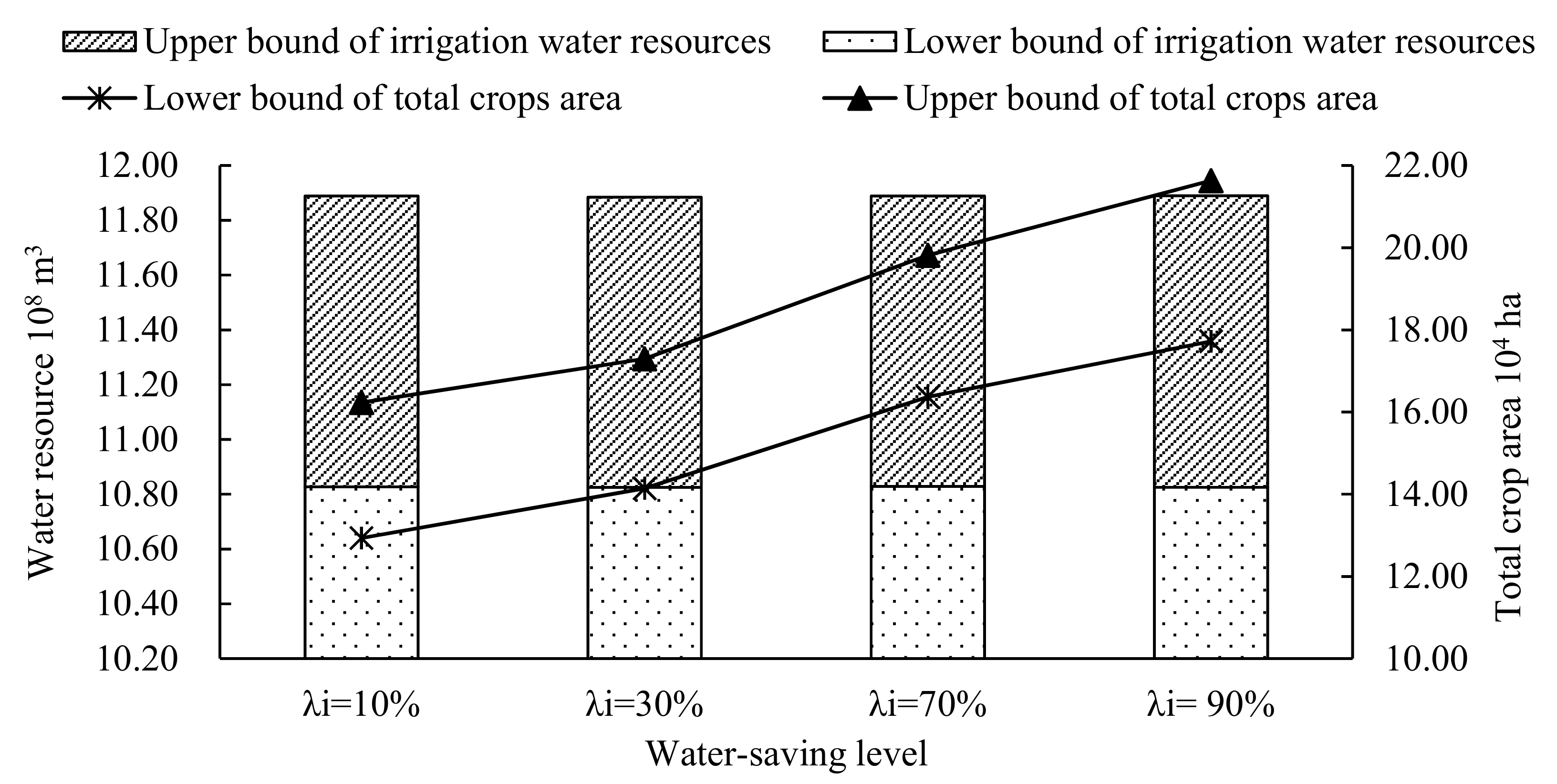
4. Analysis of the Results and Discussion
5. Conclusions
Author Contributions
Funding
Conflicts of Interest
References
- Luo, P.; Zhou, M.; Deng, H.; Lyu, J.; Cao, W.; Takara, K.; Nover, D.; Schladow, S.G. Impact of forest maintenance on water shortages: Hydrologic modeling and effects of climate change. Sci. Total Environ. 2018, 615, 1355–1363. [Google Scholar] [CrossRef] [PubMed]
- Ren, C.F.; Li, Z.H.; Zhang, H.B. Integrated multi-objective stochastic fuzzy programming and AHP method for agricultural water and land optimization allocation under multiple uncertainties. J. Clean. Prod. 2019, 210, 12–24. [Google Scholar] [CrossRef]
- Wang, S.; Huang, G.H. A multi-level Taguchi-factorial two-stage stochastic programming approach for characterization of parameter uncertainties and their interactions: An application to water resources to water resources management. Eur. J. Oper. Res. 2015, 240, 572–581. [Google Scholar] [CrossRef]
- Li, M.; Fu, Q.; Singh, V.P.; Liu, D. An interval multi-objective programming model for irrigation water allocation under uncertainty. Agric. Water Manag. 2018, 196, 24–26. [Google Scholar] [CrossRef]
- Luo, P.P.; He, B.; Duan, W.L. Impact assessment of rainfall scenarios and land-use change on hydrologic response using synthetic area IDF curves. J. Flood Risk Manag. 2018, 11, S84–S97. [Google Scholar] [CrossRef]
- Cai, X.L.; Cui, Y.L. Crop Planting structure extraction in irrigated areas from multi-sensor and multi-temporal remote sensing data. Trans. Chin. Soc. Agric. Eng. 2009, 25, 124–131. (In Chinese) [Google Scholar]
- Singh, A. Land and water management planning for increasing farm income in irrigated dry areas. Land Use Policy 2015, 42, 244–250. [Google Scholar] [CrossRef]
- Mohammed, M.; Ashim, D.G.; Pushpa, R.O. Optimal crop planning model for an existing groudwater irrigation project in Thailand. Agric. Water Manag. 1997, 33, 43–62. [Google Scholar]
- Sarker, R.A.; Quaddus, M.A. Modelling a nationwide crop planning problem using a multiple criteria decision making tool. Comput. Ind. Eng. 2002, 42, 541–553. [Google Scholar] [CrossRef]
- Belin, B.; Kodal, S. A non-linear model for farm optimization with adequate and limited water supplies application to the south-east Anatolian project (GAP) region. Agric. Water Manag. 2003, 62, 187–203. [Google Scholar]
- Gorantiwar, S.D.; Smout, I.D. Multilevel approach for optimizing land and water resources and irrigation deliveries for tertiary units in large irrigation schemes. II: Application. J. Irrig. Drain. Eng. 2005, 131, 264–272. [Google Scholar] [CrossRef]
- Singh, A. Optimizing the use of land and water resources for maximizing farm income by mitigating the hydrological imbalance. J. Hydrol. Eng. 2014, 19, 1447–1451. [Google Scholar] [CrossRef]
- Garg, N.K.; Dadhich, S.M. Integrated non-linear model for optimal cropping pattern and irrigation scheduling under deficit irrigation. Agric. Water Manag. 2014, 140, 1–13. [Google Scholar] [CrossRef]
- Chang, J.; Guo, A.; Wang, Y.; Ha, Y.; Zhang, R.; Xue, L.; Tu, Z. Reservoir operations to mitigate drought effects with a hedging policy triggered by the drought prevention limiting water level. Water Resour. Res. 2019, 55, 904–922. [Google Scholar] [CrossRef]
- Nguyen, D.C.; Dandy, G.C.; Maier, H.R.; Ascough, J.C. Improved ant colony optimization for optimal crop and irrigation water allocation by incorporating domain knowledge. J. Water Resour. Plan. Manag. 2016, 142, 04016025. [Google Scholar] [CrossRef]
- Galan-Martin, A.; Vaskan, P.; Anton, A.; Esteller, L.J.; Guillén-Gosálbez, G. Multi-objective optimization of rainfed and irrigated agricultural areas considering production and environmental criteria: A case study of wheat production in Spain. J. Clean. Prod. 2017, 140, 816–830. [Google Scholar] [CrossRef]
- Fazlali, A.; Shourian, M. A demand management based crop and irrigation planning using the simulation-optimization approach. Water Resour. Manag. 2018, 32, 67–81. [Google Scholar] [CrossRef]
- Li, M.; Fu, Q.; Singh, V.P.; Ji, Y.; Liu, D.; Zhang, C.; Li, T. An optimal modelling approach for managing agricultural water-energy-food nexus under uncertainty. Sci. Total Environ. 2019, 651, 1416–1434. [Google Scholar] [CrossRef]
- Li, M.; Fu, Q.; Singh, V.P.; Ma, M.W.; Liu, X. An intuitionistic fuzzy multi-objective non-linear programming model for sustainable irrigation water allocation under the combination of dry and wet conditions. J. Hydrol. 2017, 555, 80–94. [Google Scholar] [CrossRef]
- Hamid, R.S.; Mohammad, A.A. Optimal crop planning and conjunctive use of surface water and groundwater resources using fuzzy dynamic programming. J. Irrig. Drain. Eng. 2011, 137, 383–397. [Google Scholar]
- Tong, F.F.; Guo, P. Simulation and optimization for crop water allocation based on crop water production functions and climate factor under uncertainty. Appl. Math. Model. 2013, 37, 7708–7716. [Google Scholar] [CrossRef]
- Xie, Y.L.; Huang, G.H.; Li, W.; Li, J.B.; Li, Y.F. An inexact two-stage stochastic programming model for water resources management in Nansihu Lake Basin, China. J. Environ. Manag. 2013, 127, 188–205. [Google Scholar] [CrossRef] [PubMed]
- Wang, S.; Huang, G.H. An integrated approach for water resources decision making under interactive and compound uncertainties. Omega 2014, 44, 32–40. [Google Scholar] [CrossRef]
- Jiang, Y.; Xu, X.; Huang, Q.; Huo, Z.; Huang, G. Optimizing regional irrigation water use by integrating a two-level optimization model and an agro-hydrological model. Agric. Water Manag. 2016, 178, 76–88. [Google Scholar] [CrossRef]
- Li, Y.P.; Huang, G.H. Fuzzy-stochastic-based analysis method for planning water resources management systems with uncertain information. Inf. Sci. 2009, 179, 4261–4276. [Google Scholar] [CrossRef]
- Li, Y.P.; Liu, J.; Huang, G.H. A hybrid fuzzy-stochastic programming method for water trading within an agricultural system. Agric. Syst. 2014, 123, 71–83. [Google Scholar] [CrossRef]
- Wang, C.X.; Li, Y.P.; Huang, G.H.; Zhang, J.L. A type-2 fuzzy interval programming approach for conjunctive use of surface water and groundwater under uncertainty. Inf. Sci. 2016, 340, 209–227. [Google Scholar] [CrossRef]
- Ren, C.F.; Zhang, H.B. A fuzzy max-min decision bi-level fuzzy programming model for water resources optimization allocation under uncertainty. Water 2018, 10, 488. [Google Scholar] [CrossRef]
- Aliev, R.A.; Pedrycz, W.; Kreinovich, V.; Huseynov, O.H. The general theory of decisions. Inf. Sci. 2016, 327, 125–148. [Google Scholar] [CrossRef]
- Kundu, P.; Kar, S.; Maiti, M. Fixed charge transportation problem with type-2 fuzzy variables. Inf. Sci. 2014, 255, 170–186. [Google Scholar] [CrossRef]
- Nie, S.; Huang, C.Z.; Huang, G.H.; Li, Y.P.; Chen, J.P.; Fan, Y.R.; Cheng, G.H. Planning renewable energy in electric power system for sustainable development under uncertainty—A case study of Beijing. Appl. Energy 2016, 162, 772–786. [Google Scholar] [CrossRef]
- Li, Y.P.; Huang, G.H.; Yang, Z.F.; Nie, S.L. IFMP: Interval-fuzzy multistage programming for water resources management under uncertainty. Resour. Conserv. Recycl. 2008, 52, 800–812. [Google Scholar] [CrossRef]
- Xie, Y.L.; Xia, D.X.; Ji, L.; Huang, G.H. An inexact stochastic-fuzzy optimization model for agricultural water allocation and land resources utilization management under considering effective rainfall. Ecol. Indic. 2018, 92, 301–311. [Google Scholar] [CrossRef]
- Zhu, H.; Huang, G.H. SLFP: A stochastic linear fractional programming approach for sustainable waste management. Waste Manag. 2011, 31, 2612–2619. [Google Scholar] [CrossRef] [PubMed]
- Ren, C.F.; Guo, P.; Li, M.; Gu, J.J. Optimization of industrial structure considering the uncertainty of water resources. Water Resour. Manag. 2013, 27, 3885–3898. [Google Scholar] [CrossRef]
- Ren, C.F.; Li, R.H.; Zhang, L.D.; Guo, P. Multiobjective stochastic fractional goal programming model for water resources optimal allocation among industries. J. Water Resour. Plan. Manag. 2016, 142, 04016036. [Google Scholar] [CrossRef]
- Ren, C.F.; Guo, P.; Tian, Q.; Zhang, L.D. A multi-objective fuzzy programming model for optimal use of irrigation water and land resources under uncertainty in Gansu Province, China. J. Clean. Prod. 2017, 164, 85–94. [Google Scholar] [CrossRef]
- Zara, Y.; Daneshmand, A. A linear approximation method for solving a special class of the chance constrained programming problem. Eur. J. Oper. Res. 1995, 80, 213–225. [Google Scholar] [CrossRef]
- Charnes, A.; Cooper, W.W.; Kriby, P. Chance constrained programming an extension of statistical method. In Optimizing Methods in Statistics; Academic Press: New York, NY, USA, 1972; pp. 391–402. [Google Scholar]
- Gui, Z.Y.; Li, M.; Guo, P. Simulation-based inexact fuzzy semi-infinite programming method for agricultural cultivated area planning in the Shiyang River Basin. J. Irrig. Drain. Eng. 2016, 143, 05016001. [Google Scholar] [CrossRef]
- Xu, W.H.; Zhong, Y.M.; Chen, G. The state of the art in water resources utilization in Shiyang River Basin and the countermeasures for sustainable utilization. J. Glaciol. Geocryol. 2007, 2, 36–40. [Google Scholar]
- Huang, Y.; Li, Y.P.; Chen, X.; Ma, Y.G. Optimization of the irrigation water resources for agricultural sustainability in Tarim river basin, China. Agric. Water Manag. 2012, 107, 74–85. [Google Scholar] [CrossRef]


| Crops | Yield (kg/ha) | Irrigation Quota (m3/ha) | ET (m3/ha) | P (¥/ha) | C (¥/ha) | Amin (ha) | Amax (ha) | |||
|---|---|---|---|---|---|---|---|---|---|---|
| Mode 1 | Mode 2 | Mode 1 | Mode 2 | Mode 1 | Mode 2 | |||||
| Wheat | (5447, 5745) | (5175, 5250) | (5150, 5250) | (4150, 4450) | (5410, 6490) | (4050, 4500) | (1.8, 2) | 7179.5 | 0.9396 | 4.2282 |
| Maize | (10,470, 10,695) | (12,750, 12,750) | (5400, 5520) | (3000, 3600) | (5400, 5520) | (3000, 3600) | (1.3, 1.5) | 7788 | 1.8782 | 8.4519 |
| Bean | (2482, 2884) | (2482, 2884) | (3950, 4450) | (3950, 4450) | (5715, 5715) | (5715, 5715) | 4 | 5500 | 0.0866 | 0.3897 |
| Potato | (27,000, 30,000) | 33,000 | (4370, 4850) | (3500, 3640) | (5200, 5705) | (4213, 4270) | (0.5, 0.6) | 5250 | 0.7768 | 3.4956 |
| Maize seed | (14,041, 14,428) | (13,835, 15,418) | (2250, 3250) | (2250, 2250) | (3621, 4248) | (3617, 3500) | 2.2 | 16,075.5 | 0.2386 | 1.0737 |
| Cotton | (1800, 1845) | (1980, 2030) | (3950, 4450) | (1950, 3150) | (3440, 4300) | (3600, 4695) | (5, 5.5) | 5235 | 0.1500 | 0.6750 |
| Oilseed | (3559, 3674) | (3559, 3674) | (4800, 5250) | (4800, 5250) | (3750, 4695) | (3750, 4695) | (3, 3.4) | 3650 | 0.8018 | 3.6351 |
| Vegetable | 11,5500 | 11,3250 | (4500, 5300) | (2680, 3100) | (5400, 6450) | (2200, 2900) | (1, 1.3) | 18,000 | 1.3540 | 6.0930 |
| Cucurbit | 60,882 | 63,196 | (4200, 4800) | (2700, 3150) | (3900, 4190) | (3300, 3670) | 1.8 | 9125 | 0.1212 | 0.5454 |
| Apple | 11,545 | 11,545 | (4780, 5290) | (4780, 5290) | (5825, 6742) | (5825, 6742) | (2, 2.2) | 4950 | 0.2050 | 0.9225 |
| Grape | (13,500, 15,000) | 12,000 | 4130 | 2130 | (4296, 5000) | (3017, 3073) | (3, 3.5) | 8000 | 0.2670 | 1.2015 |
| TA (104 ha) | TPR (104 P) | FDP (kg/P) | SW (104 m3) | EW (104 m3) | DW (104 m3) | TW (104 m3) | IC |
|---|---|---|---|---|---|---|---|
| 24.28 | 186.14 | 300 | 21,838.5 | 15,544.8 | 5832.67 | 2261.57 | 0.59 |
© 2019 by the authors. Licensee MDPI, Basel, Switzerland. This article is an open access article distributed under the terms and conditions of the Creative Commons Attribution (CC BY) license (http://creativecommons.org/licenses/by/4.0/).
Share and Cite
Ren, C.; Zhang, H. An Inexact Optimization Model for Crop Area Under Multiple Uncertainties. Int. J. Environ. Res. Public Health 2019, 16, 2610. https://doi.org/10.3390/ijerph16142610
Ren C, Zhang H. An Inexact Optimization Model for Crop Area Under Multiple Uncertainties. International Journal of Environmental Research and Public Health. 2019; 16(14):2610. https://doi.org/10.3390/ijerph16142610
Chicago/Turabian StyleRen, Chongfeng, and Hongbo Zhang. 2019. "An Inexact Optimization Model for Crop Area Under Multiple Uncertainties" International Journal of Environmental Research and Public Health 16, no. 14: 2610. https://doi.org/10.3390/ijerph16142610
APA StyleRen, C., & Zhang, H. (2019). An Inexact Optimization Model for Crop Area Under Multiple Uncertainties. International Journal of Environmental Research and Public Health, 16(14), 2610. https://doi.org/10.3390/ijerph16142610