Identifying the Driving Factors of Black Bloom in Lake Bay through Bayesian LASSO


Abstract
:1. Introduction
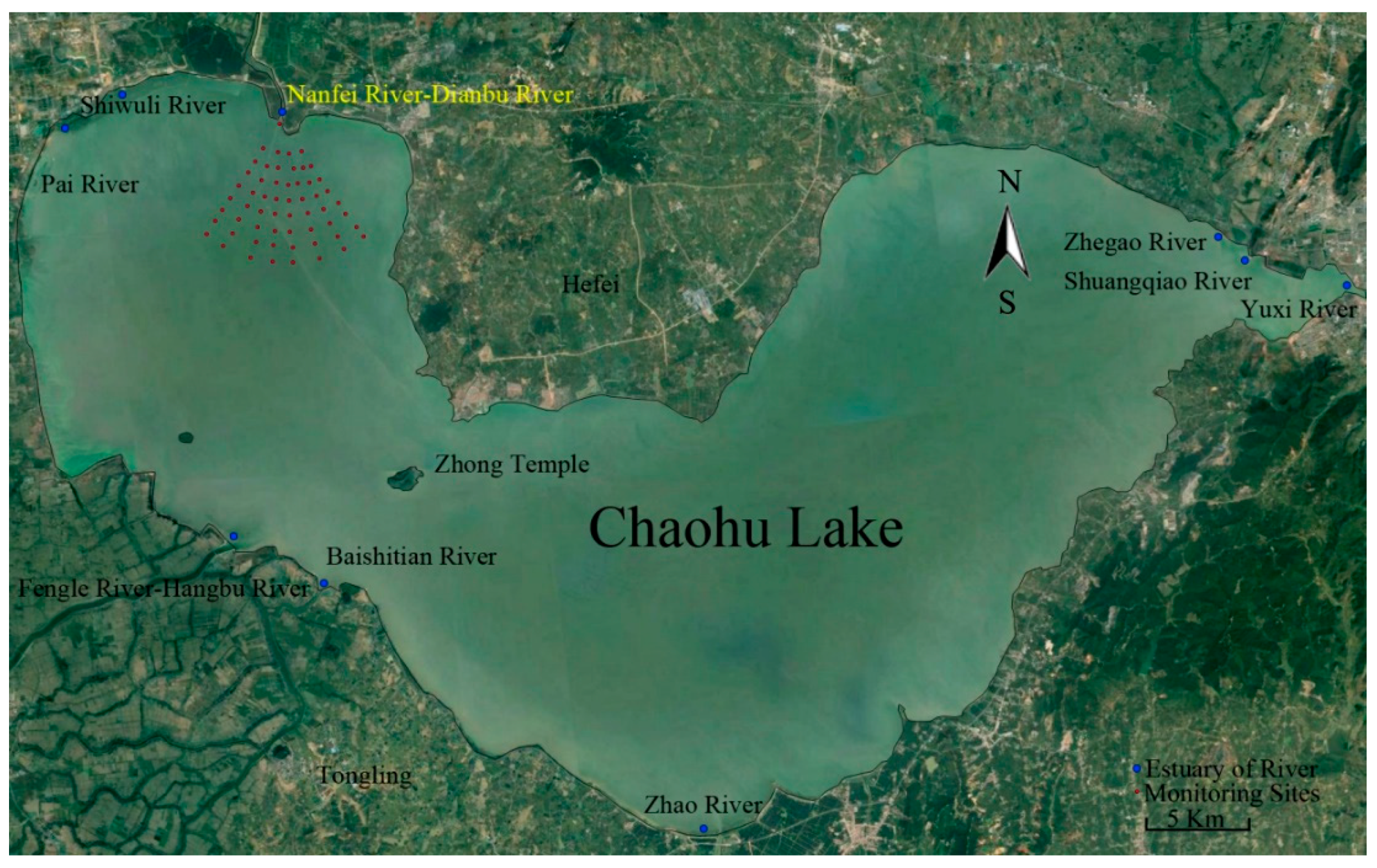
2. Research Region and Data
3. Methods
4. Results and Discussion
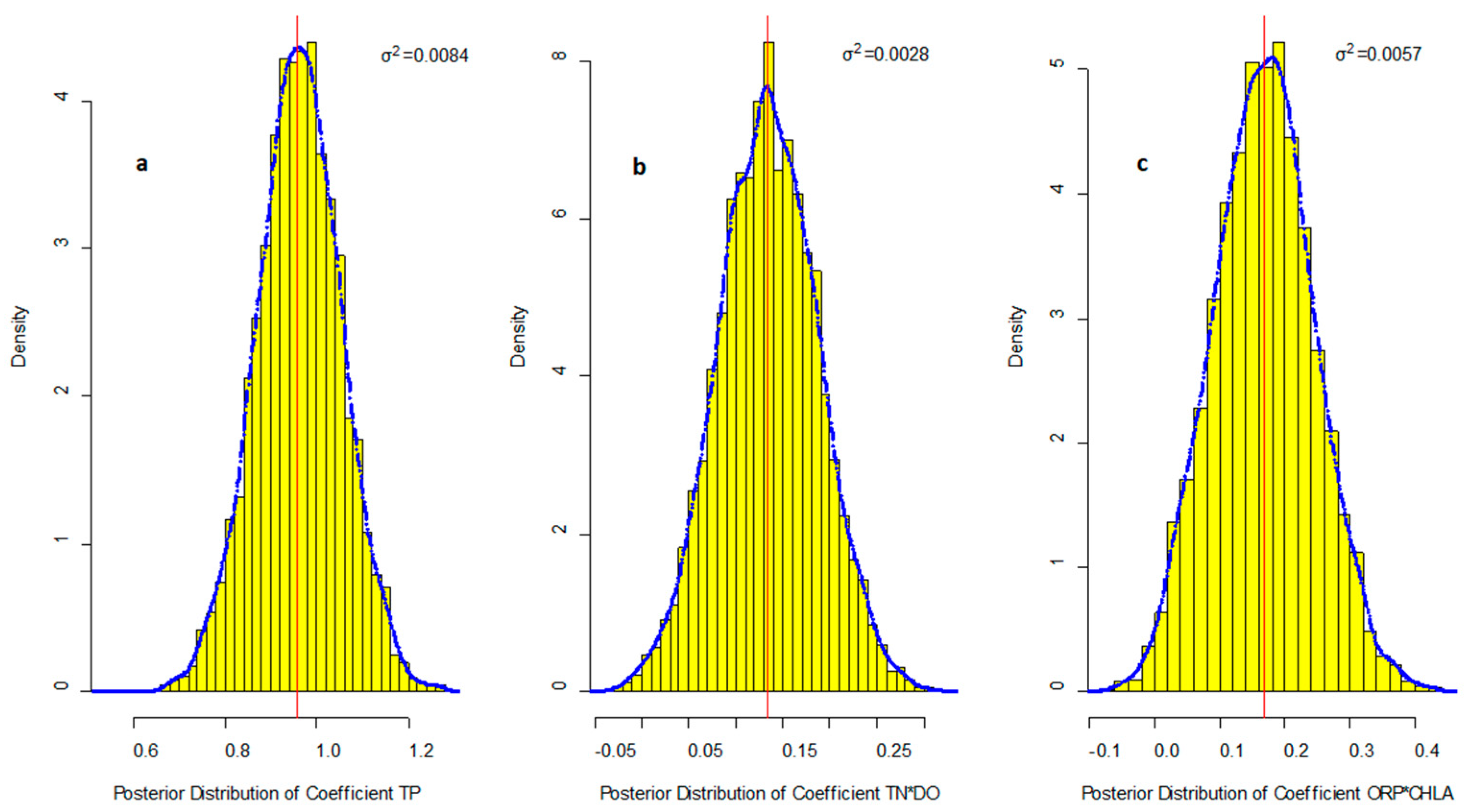
R2 = 0.841, Adjust R2 = 0.832, at α = 0.05 significance level (p < 0.05)
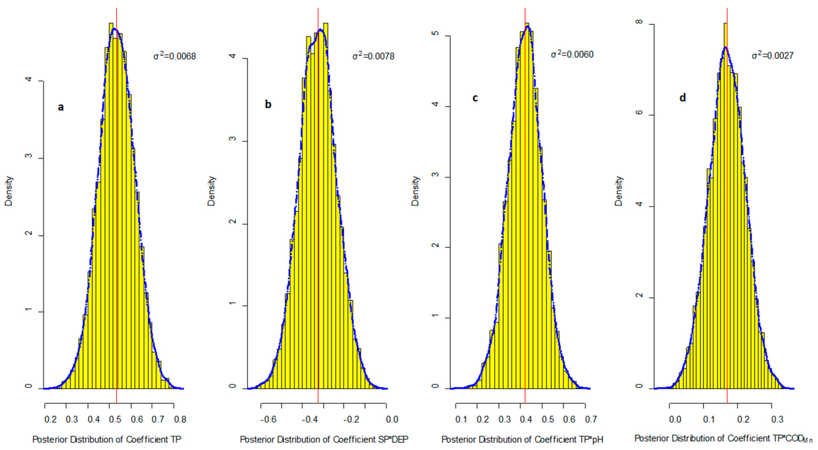
R2 = 0.628, Adjust R2 = 0.602. at α = 0.05 significance level (p < 0.005)
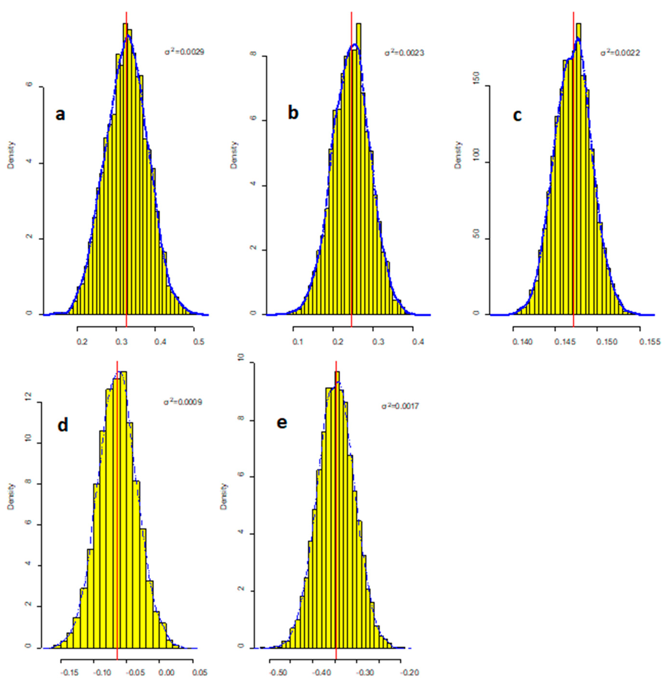
R2 = 0.796, Adjusted R2 = 0.778, at α = 0.05 significance level (p < 0.05)
5. Conclusions
Author Contributions
Funding
Acknowledgments
Conflicts of Interest
References
- Fan, C.X. Progress and Prospect in Formation of Black Bloom in Lake Taihu: A Review. J. Lake Sci. 2015, 27, 553–566. [Google Scholar]
- Stahl, J.B. Black Water and Two Peculiar Types of Stratification in an Organically Loaded Strip-Mine Lake. Water Res. 1979, 13, 467–471. [Google Scholar] [CrossRef]
- Duval, B.; Ludlam, S.D. The Black Water Chemocline of Meromictic Lower Mystic Lake, Massachusetts, USA. Int. Rev. Hydrobiol. 2001, 86, 165–181. [Google Scholar] [CrossRef]
- Sandra, P.; Federico, B.; Giovanna, P.; Sabrina, P.; Patrizia, B.; Cristina, M. Biomonitoring of Lake Garda: Identification of Ciliate Species and Symbiotic Algae Responsible for the Black-Spot Bloom During the Summer of 2004. Environ. Res. 2008, 107, 194–200. [Google Scholar]
- Guo, L. Doing Battle with the Green Monster of Taihu Lake. Science 2007, 317, 1166. [Google Scholar] [CrossRef]
- Deng, X.W.; Tao, M.; Zhang, L.; Xie, P.; Chen, J.; Zhang, J. Relationships between Odors and Algae and Water Quality in Dongting Lake. Res. Envrion. Sci. 2013, 26, 16–21. [Google Scholar]
- Rai, H.; Hill, G. Physical and Chemical Studies of Lago TupÉ: A Central Amazonian Black Water &Ldquo;Ria Lake&Rdquo. Int. Rev. Gesam. Hydrobiol. 1981, 66, 37–82. [Google Scholar]
- Lazaro, T.R. Urban Hydrogy; Ann Arbor Science Publishers Inc.: Ann Arbor, MI, USA, 1979. [Google Scholar]
- Lu, G.H.; Ma, Q.; Zhang, J.H. Analysis of Black Water Aggregation in Taihu Lake. Water Sci. Eng. 2011, 4, 374–385. [Google Scholar]
- Shi, K.; Zhang, Y.L.; Zhou, Y.Q.; Liu, X.H.; Zhu, G.W.; Qin, B.Q.; Gao, G. Long-Term Modis Observations of Cyanobacterial Dynamics in Lake Taihu: Responses to Nutrient Enrichment and Meteorological Factors. Sci. Rep. 2017, 7, 40326. [Google Scholar] [CrossRef]
- Liu, J.J.; Lu, J.; Zhu, G.W.; Gao, M.Y.; Wen, L.; Yao, M.; Nie, Q. Occurence Characteristics of Black Patch Events and Their Influencing Factors in Lake Taihu During 2009 and 2017. J. Lake Sci. 2018, 30, 1196–1205. [Google Scholar]
- Shen, A.C.; Xu, Z.A.; Wu, D.H. Relationships between Accumulation and Dying of Cyanobacteria and Black Spot. J. Hydroecol. 2012, 33, 68–72. [Google Scholar]
- Cheng, X.; Earl, P.; Burlingame, G.A. A Study on Volatile Organic Sulfide Causes of Odors at Philadelphia’s Northeast Water Pollution Control Plant. Water Res. 2005, 39, 3781–3790. [Google Scholar] [CrossRef] [PubMed]
- Han, C.; Ding, S.; Yao, L.; Shen, Q.; Zhu, C.; Wang, Y.; Xua, D. Dynamics of Phosphorus-Iron-Sulfur at the Sediment-Water Interface Influenced by Algae Blooms Decomposition. J. Hazard. Mater. 2015, 300, 329–337. [Google Scholar] [CrossRef] [PubMed]
- Wang, C.L.; Zhang, Y.; Zhang, N.H.; Qian, X.; Kong, F.X. Analysis of Meteorological Factors of Forming Feculent and Anaerobic Water Aggreation Induced by Algal Bloom in Taihu Lake. Environ. Sci. 2011, 32, 401–408. [Google Scholar]
- Jiang, X.; Lu, W.X.; Zhao, H.Q.; Yang, Q.C.; Mo, C. Quantitative Evaluation of Mining Geo-Environmental Quality in Northeast China: Comprehensive Index Method and Support Vector Machine Models. Environ. Ear. Sci. 2015, 73, 7945–7955. [Google Scholar] [CrossRef]
- Shen, Q.S.; Fan, C.X.; Liu, C.; Chen, C. The Limiting Factor to the Outbreak of Lake Black Bloom: Roles of Ferrous Iron and Sulfide Ions. Clean Soil Air Water 2018, 46, 1800305. [Google Scholar] [CrossRef]
- Lu, X.; Fan, C.X.; He, W.; Deng, J.C.; Yin, H.B. Sulfur-Containing Amino Acid Methionine as the Precursor of Volatile Organic Sulfur Compounds in Algea-Induced Black Bloom. J. Environ. Sci. 2013, 25, 33–43. [Google Scholar] [CrossRef]
- Fan, C.X.; Shen, Q.S. Identification of Black Suspended Particles in the Algae-Induced Black Bloom Water Column. J. Lake Sci. 2015, 25, 591–598. [Google Scholar]
- Canfield, D.E., Jr.; Linda, S.B.; Hodgson, L.M. Relations between Color and Some Limnological Characteristics of Florida Lakes. JAWRA 1984, 20, 323–329. [Google Scholar]
- Sugiura, N.; Utsumi, M.; Wei, B.; Iwami, N.; Okano, K.; Kawauchi, Y.; Maekawa, T. Assessment for the Complicated Occurrence of Nuisance Odours from Phytoplankton and Environmental Factors in a Eutrophic Lake. Lakes Reserv. Res. Manag. 2004, 9, 195–201. [Google Scholar] [CrossRef]
- Dzialowski, A.R.; Smith, V.H.; Huggins, D.G.; deNoyelles, F.; Lim, N.C.; Baker, D.S.; Beury, J.H. Development of Predictive Models for Geosmin-Related Taste and Odor in Kansas, USA, Drinking Water Reservoirs. Water Res. 2009, 43, 2829–2840. [Google Scholar] [CrossRef] [PubMed]
- Liu, G.F.; Shen, Q.S.; Zhang, L.; Fan, C.X.; Zhong, J.C.; Yan, S.H. Environment Effects of Algae-Caused Black Spots: Driving Effects on the N,P Changes in the Water-Sediment Interface. Environ. Sci. 2010, 31, 2917–2924. [Google Scholar]
- Liu, G.F.; He, J.; Fan, C.X.; Zhang, L.; Shen, Q.S.; Zhong, J.C.; Yan, S.H. Environment Effects of Algae-Caused Black Spots: Impacts on Fe-Mn-S Cycles in Water-Sediment Interface. Environ. Sci. 2010, 31, 2652–2660. [Google Scholar]
- Liu, G.F.; Fan, C.X.; Zhang, L.; Shen, Q.S.; Wang, Z.D.; Han, S.Q. Environment Effects of Algae-Caused Black Spots Iii: Impacts on Fe-S-P Cycle in Water-Sediment Interface. China Environ. Sci. 2014, 34, 3199–3206. [Google Scholar]
- Wang, Y.L.; Wang, L.; Hua, Z.L. The Relationships of Different Concentration Fe2+, S2− with Hydrodynamics, Do in Black Bloom Water Based on Quantile Regression Method. China Environ. Sci. 2018, 38, 627–633. [Google Scholar]
- Wang, Y.L.; Wang, L.; Hua, Z.L.; Ding, S.M. The Relationships of Velocity, Dissolved Oxygen with Fe2+, S2− in Black Bloom Region on Nanfei River Estuary of Lake Chaohu. J. Lake Sci. 2016, 28, 710–717. [Google Scholar]
- Gelman, A.; Carlin, J.B.; Stern, H.S.; Dunson, D.B.; Vehtari, A.; Rubin, D.B. Bayesian Data Analysis; CRC Press: New York, NY, USA, 2013; pp. 1–28. [Google Scholar]
- Hastie, T.; Tibshirani, R.; Wainwright, M. Statistical Learning with Sparsity: The Lasso and Generalizations; CRC Press: New York, NY, USA, 2015; pp. 139–142. [Google Scholar]
- Tibshiran, R. Regression Shrinkage and Selection Via the Lasso. J. R. Stat. Soc. B 1996, 73, 267–288. [Google Scholar] [CrossRef]
- Stookey, L.L. Ferrozine-a New Spectrophotometric Reagent for Iron. Anal. Chem. 1970, 42, 779–781. [Google Scholar] [CrossRef]
- Wei, F. Mornitoring and Analytic Method for Water and Waste Water; China Environmental Publisher: Beijing, China, 2002; pp. 88–129. [Google Scholar]
- Cline, J.D. Spectrophotometric Determination of Hydrogen Sulfide in Natural Waters. Limnol. Oceanogr. 1969, 14, 454. [Google Scholar] [CrossRef]
- Park, T.; Casella, G. The Byesian Lasso. J. Am. Stat. Assoc. 2008, 103, 681–686. [Google Scholar] [CrossRef]
- Yi, N.; Xu, S. Bayesian Lasso for Quantitative Trait Loci Mapping. Genetics 2008, 179, 1045–1055. [Google Scholar] [CrossRef] [PubMed]
- Hans, C. Bayesian Lasso Regression. Biome 2009, 96, 835–845. [Google Scholar] [CrossRef]
- Mutshinda, C.M.; Sillanpää, M.J. Extended Bayesian Lasso for Multiple Quantitative Trait Loci Mapping and Unobserved Phenotype Prediction. Genetics 2010, 186, 1067–1075. [Google Scholar] [CrossRef] [PubMed]
- Mutshinda, C.M.; Sillanpää, M.J. A Decision Rule for Quantitative Trait Locus Detection under the Extended Bayesian Lasso Model. Genetics 2012, 192, 1483–1491. [Google Scholar] [CrossRef] [PubMed]
- Huang, A.H.; Xu, S.Z.; Cai, X.D. Empirical Bayesian Elastic Net for Multiple Quantitative Trait Locus Mapping. Heredi 2015, 114, 107–115. [Google Scholar] [CrossRef] [PubMed]
- Base, K.; Mallick, B.K. Gene Selection Using a Two-Level Hierachical Bayesian Model. Bioinformatics 2004, 20, 3423–3430. [Google Scholar]
- Xu, S. An Empirical Bayes Method for Estimating Epistatic Effects of Quantitative Trait Loci. Biometrics 2007, 63, 513–521. [Google Scholar] [CrossRef]
- Cai, X.D.; Huang, A.H.; Xu, S.Z. Fast Empirical Bayesian Lasso for Multiple Quantitative Trait Locus Mapping. BMC Bioinform. 2011, 12, 211. [Google Scholar] [CrossRef]
- R Development Core Team. R: A Language and Environment for Statistical Computing; R Foundation for Statistical Computing: Vienna, Austria, 2016. [Google Scholar]
- Carlos, N.; Michanel, R. Black Spots Produced by Buried Macroalgae in Intertidal Sandy Sediments of the Wadden Sea: Effects on the Meiobenthos. J. Sea Res. 1996, 36, 150–170. [Google Scholar]
- Lu, G.H.; Ma, Q. Monitoring and Analysis on Black Water Aggregation in Lake Taihu, 2009. J. Lake Sci. 2010, 22, 481–487. [Google Scholar]
- Rickard, D. The Solubility of Fes. Geochim. Cosmochim. Acta 2006, 70, 5779–5789. [Google Scholar] [CrossRef]
- Di Toro, D.M.; Mahony, J.D.; Gonzalez, A.M. Particle Oxidation Model of Synthetic Fes and Sediment Acid-Volatile Sulfide. Envrion. Toxicol. Chem. 1996, 15, 2156–2167. [Google Scholar] [CrossRef]
- Baikova, I.S.; Shtamm, E.V.; Vichutinskaya, E.V.; Skurlatov, Y.I. The Mechanism of Oxidation of Fes Nanoparticles by Molecular Oxygen and Hydrogen Peroxide in Dilute Aqueous Solutions. Russ. J. Phys. Chem. B 2009, 3, 251–256. [Google Scholar] [CrossRef]


| Aquatic Factors | Maximum Value | Mean Value | Minimum Value | SD |
|---|---|---|---|---|
| Fe(II) (mg/L) | 5.51 | 1.27 | 0.24 | 0.96 |
| S(-II) (mg/L) | 0.15 | 0.04 | 0.02 | 0.02 |
| SSC (mg/L) | 1188.00 | 114.41 | 4.00 | 192.45 |
| TN (mg/L) | 4.84 | 2.17 | 0.33 | 1.18 |
| TP (mg/L) | 1.48 | 0.37 | 0.09 | 0.27 |
| SP (mg/L) | 0.42 | 0.11 | 0.02 | 0.08 |
| DO (mg/L) | 8.43 | 6.88 | 3.84 | 0.99 |
| CHLA (μg/L) | 170 | 53 | 21 | 31 |
| CODMn (mg/L) | 110.86 | 77.96 | 68.76 | 7.06 |
| ORP (mV) | 168 | 131.13 | 73 | 25.33 |
| TEMP (℃) | 28.80 | 25.35 | 23.80 | 1.84 |
| DEP (m) | 1.7 | 1.21 | 0.9 | 0.15 |
| VEL (cm/s) | 56.00 | 11.04 | 1.20 | 8.05 |
| pH | 8.35 | 8.04 | 7.22 | 0.24 |
| Aquatic Factors | Fe(II) | S(−II) | SSC | TN | TP | SP | DO | CHLA | CODMn | ORP | TEP | DEP | VEL | pH |
|---|---|---|---|---|---|---|---|---|---|---|---|---|---|---|
| Fe(II) | 1 | |||||||||||||
| S(−II) | 0.72 ** | 1 | ||||||||||||
| SSC | 0.87 ** | 0.83 ** | 1 | |||||||||||
| TN | 0.50 ** | 0.41 ** | 0.49 ** | 1 | ||||||||||
| TP | 0.76 ** | 0.68 ** | 0.80 ** | 0.78 ** | 1 | |||||||||
| SP | 0.39 ** | 0.26 * | 0.37 ** | 0.62 ** | 0.73 ** | 1 | ||||||||
| DO | −0.18 | 0.05 | −0.04 | −0.40 ** | −0.34 ** | −0.51 ** | 1 | |||||||
| CHLA | −0.03 | 0.04 | 0.02 | 0.23 | 0.08 | −0.04 | 0.18 | 1 | ||||||
| CODMn | 0.35 ** | 0.41 ** | 0.41 ** | 0.58 ** | 0.58 ** | 0.52 ** | −0.27 * | 0.20 | 1 | |||||
| ORP | −0.21 | 0.07 | −0.05 | −0.26 * | −0.09 | 0.07 | 0.24 | −0.03 | −0.12 | 1 | ||||
| TEP | −0.15 | −0.06 | 0.00 | −0.15 | −0.09 | 0.07 | −0.13 | 0.04 | 0.04 | 0.37 ** | 1 | |||
| DEP | −0.36 ** | −0.28 * | −0.34 ** | −0.27 * | −0.38 ** | −0.17 | 0.07 | 0.03 | −0.24 | 0.38 ** | 0.20 | 1 | ||
| VEL | −0.02 | 0.02 | 0.00 | −0.03 | 0.06 | 0.12 | 0.11 | 0.00 | −0.11 | 0.44 ** | 0.18 | 0.14 | 1 | |
| pH | −0.15 | 0.14 | 0.06 | −0.20 | −0.11 | −0.17 | 0.68 ** | 0.10 | −0.24 | 0.67 ** | 0.20 | 0.24 | 0.33 ** | 1 |
| Response Variables | Optimal Hyperparameters | Cross Validation Criterions | ||
|---|---|---|---|---|
| a | b | MSE * | SE ** | |
| Fe(II) | −0.60 | 0.50 | 0.45 | 0.40 |
| S(-II) | −0.10 | 0.50 | 0.94 | 1.46 |
| SSC | 0.01 | 0.10 | 0.20 | 0.18 |
© 2019 by the authors. Licensee MDPI, Basel, Switzerland. This article is an open access article distributed under the terms and conditions of the Creative Commons Attribution (CC BY) license (http://creativecommons.org/licenses/by/4.0/).
Share and Cite
Wang, L.; Wang, Y.; Cheng, H.; Cheng, J. Identifying the Driving Factors of Black Bloom in Lake Bay through Bayesian LASSO. Int. J. Environ. Res. Public Health 2019, 16, 2492. https://doi.org/10.3390/ijerph16142492
Wang L, Wang Y, Cheng H, Cheng J. Identifying the Driving Factors of Black Bloom in Lake Bay through Bayesian LASSO. International Journal of Environmental Research and Public Health. 2019; 16(14):2492. https://doi.org/10.3390/ijerph16142492
Chicago/Turabian StyleWang, Liang, Yulin Wang, Haomiao Cheng, and Jilin Cheng. 2019. "Identifying the Driving Factors of Black Bloom in Lake Bay through Bayesian LASSO" International Journal of Environmental Research and Public Health 16, no. 14: 2492. https://doi.org/10.3390/ijerph16142492
APA StyleWang, L., Wang, Y., Cheng, H., & Cheng, J. (2019). Identifying the Driving Factors of Black Bloom in Lake Bay through Bayesian LASSO. International Journal of Environmental Research and Public Health, 16(14), 2492. https://doi.org/10.3390/ijerph16142492