Multi-Temporal Effects of Urban Forms and Functions on Urban Heat Islands Based on Local Climate Zone Classification

Abstract
1. Introduction
2. Study Area and Data
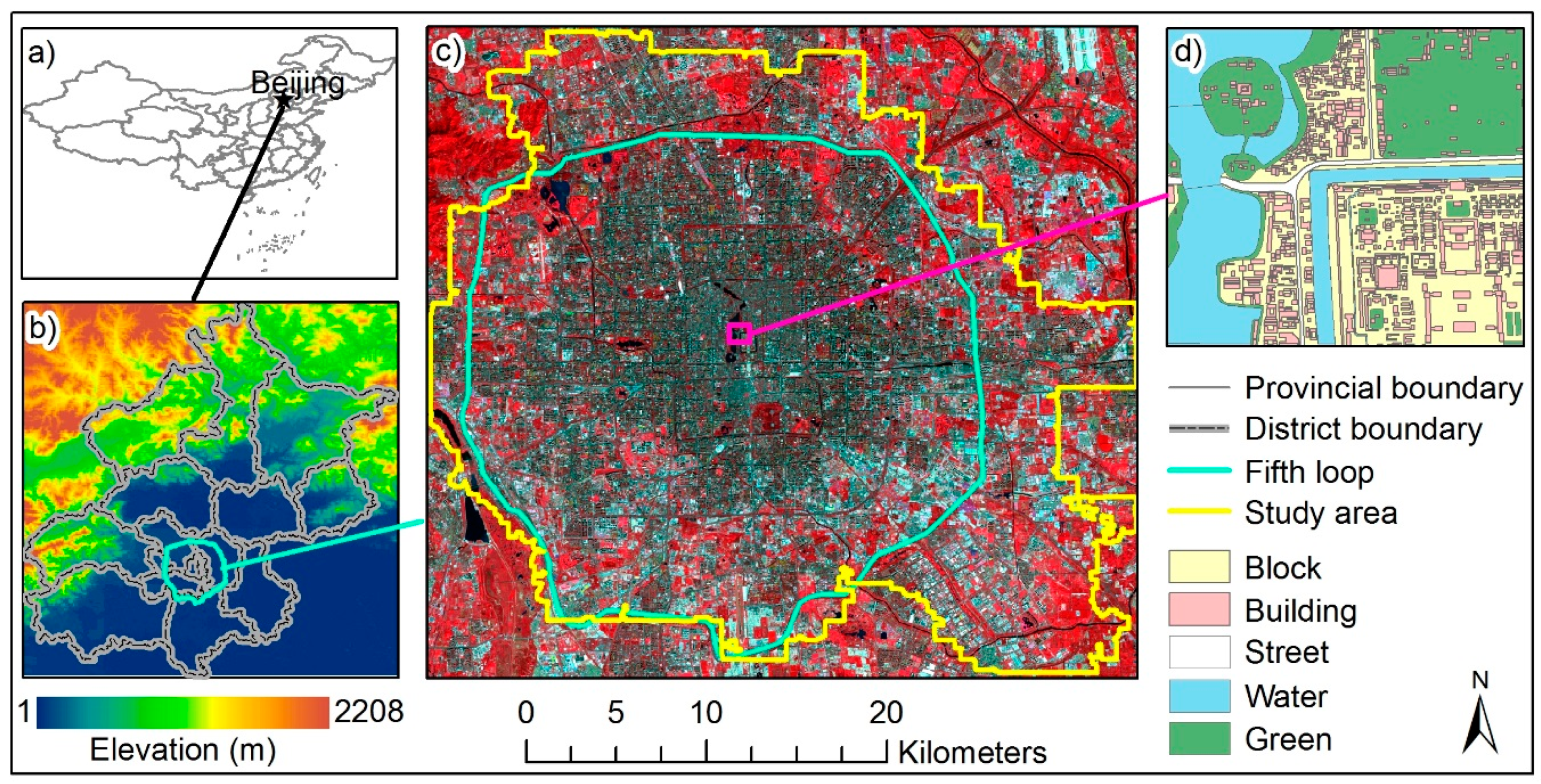
2.1. Study Area
2.2. Data
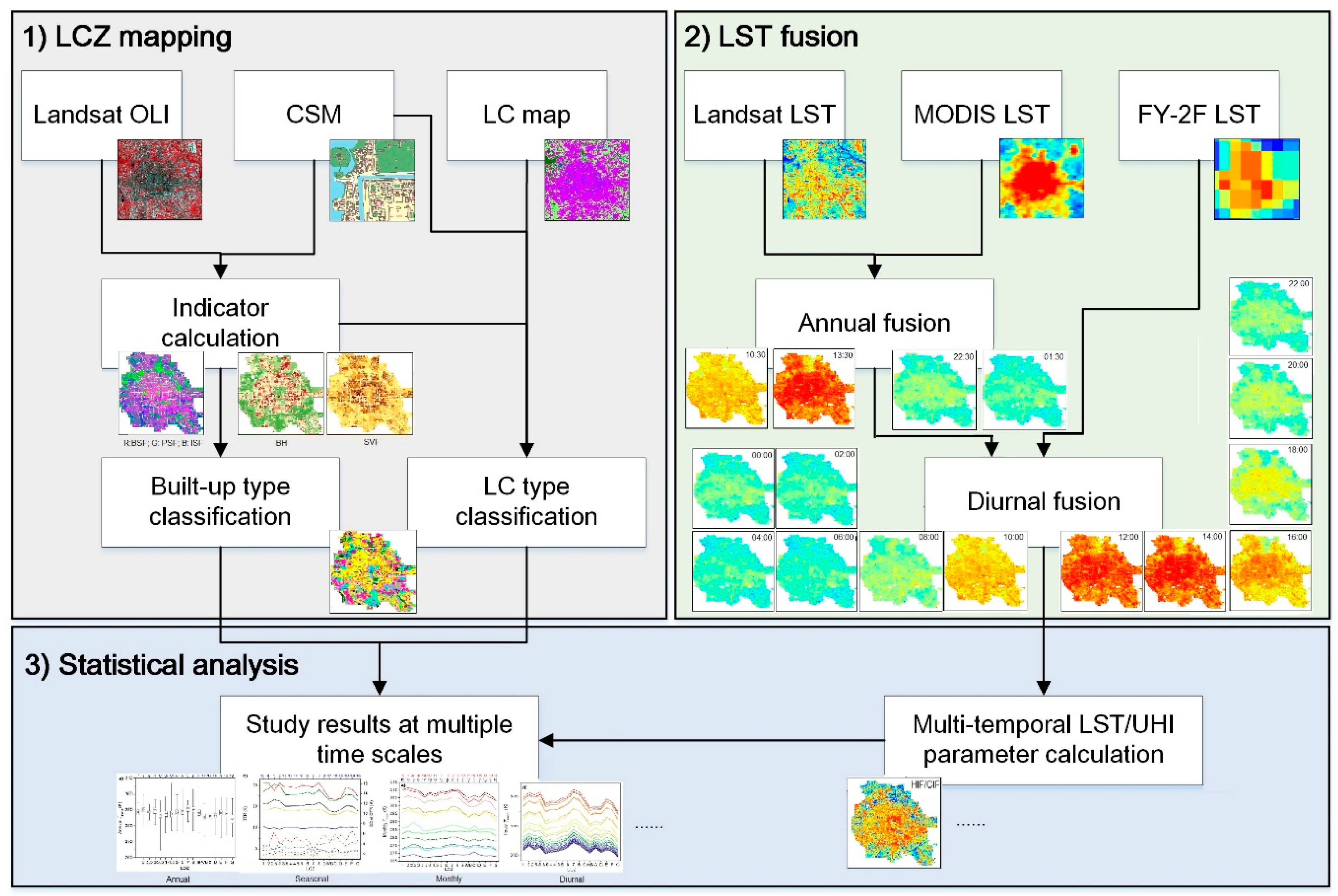
3. Methods
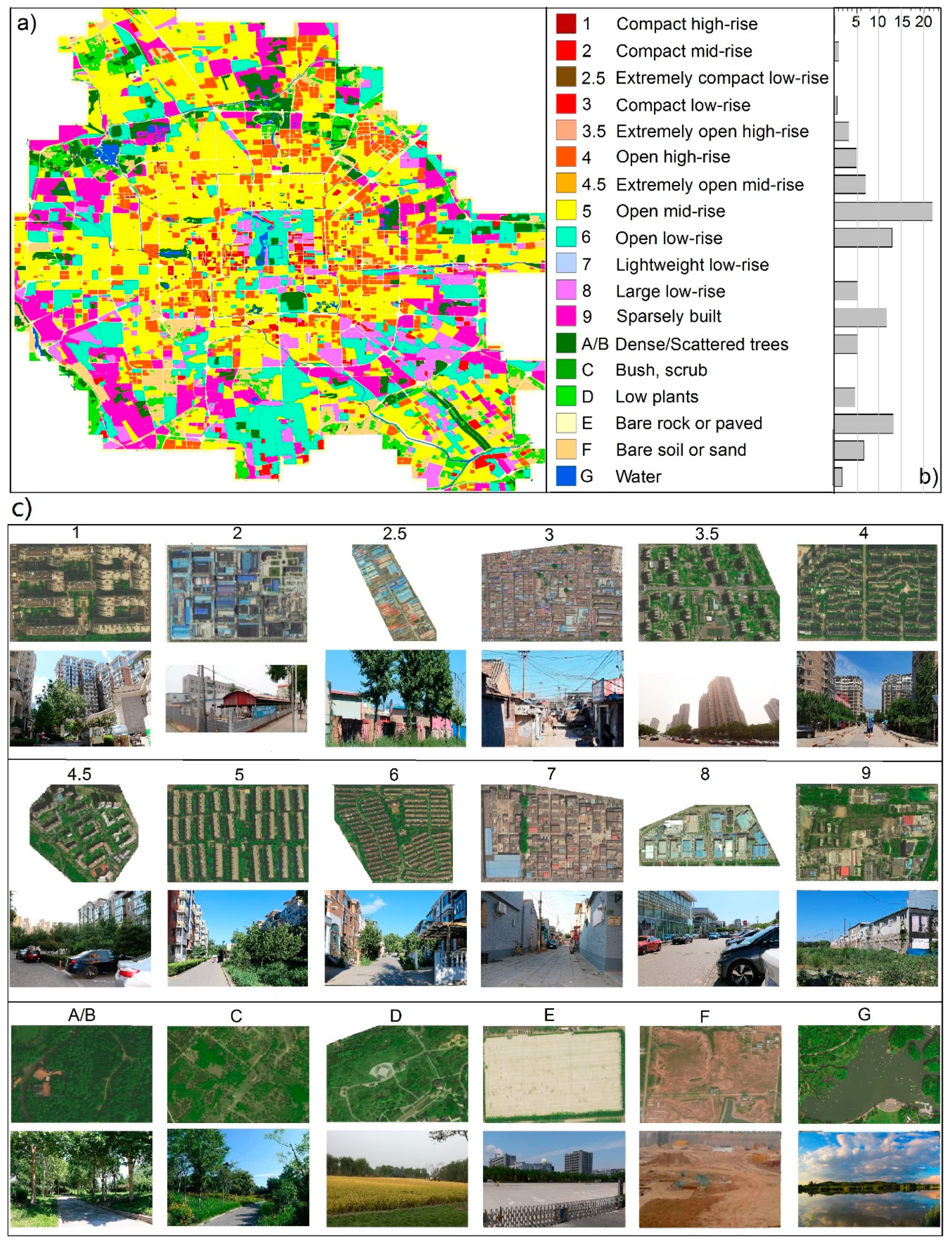
3.1. Local Climate Zone Mapping
3.2. Land Surface Temperature Fusion
3.3. Statistical Analysis
4. Results
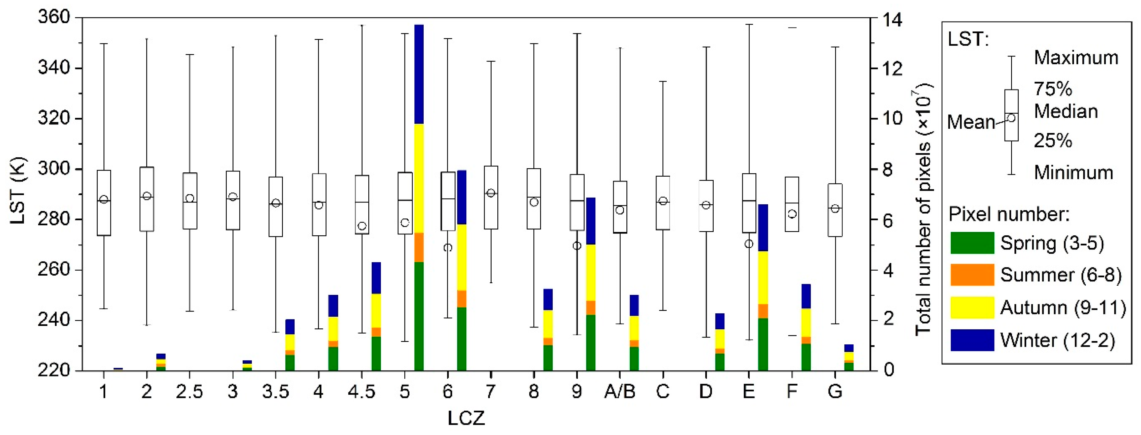
4.1. A General View of the Local Climate Zones and Land Surface Temperatures
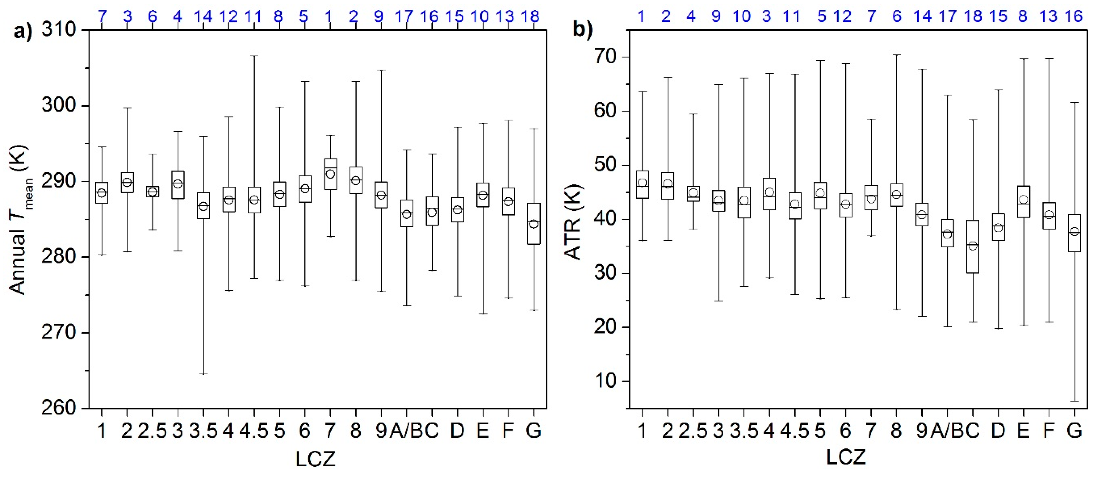
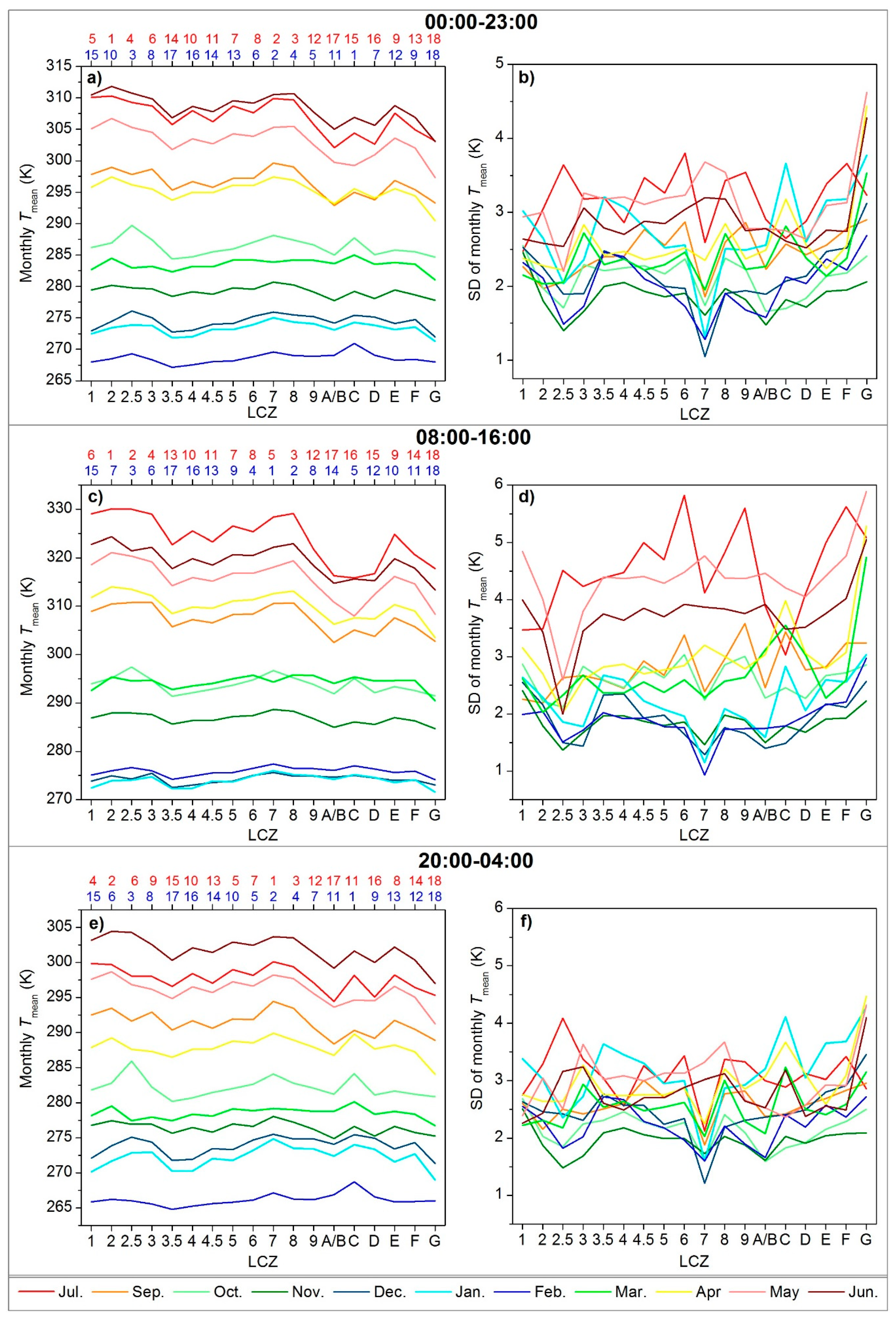
4.2. Annual and Monthly Land Surface Temperature Variations
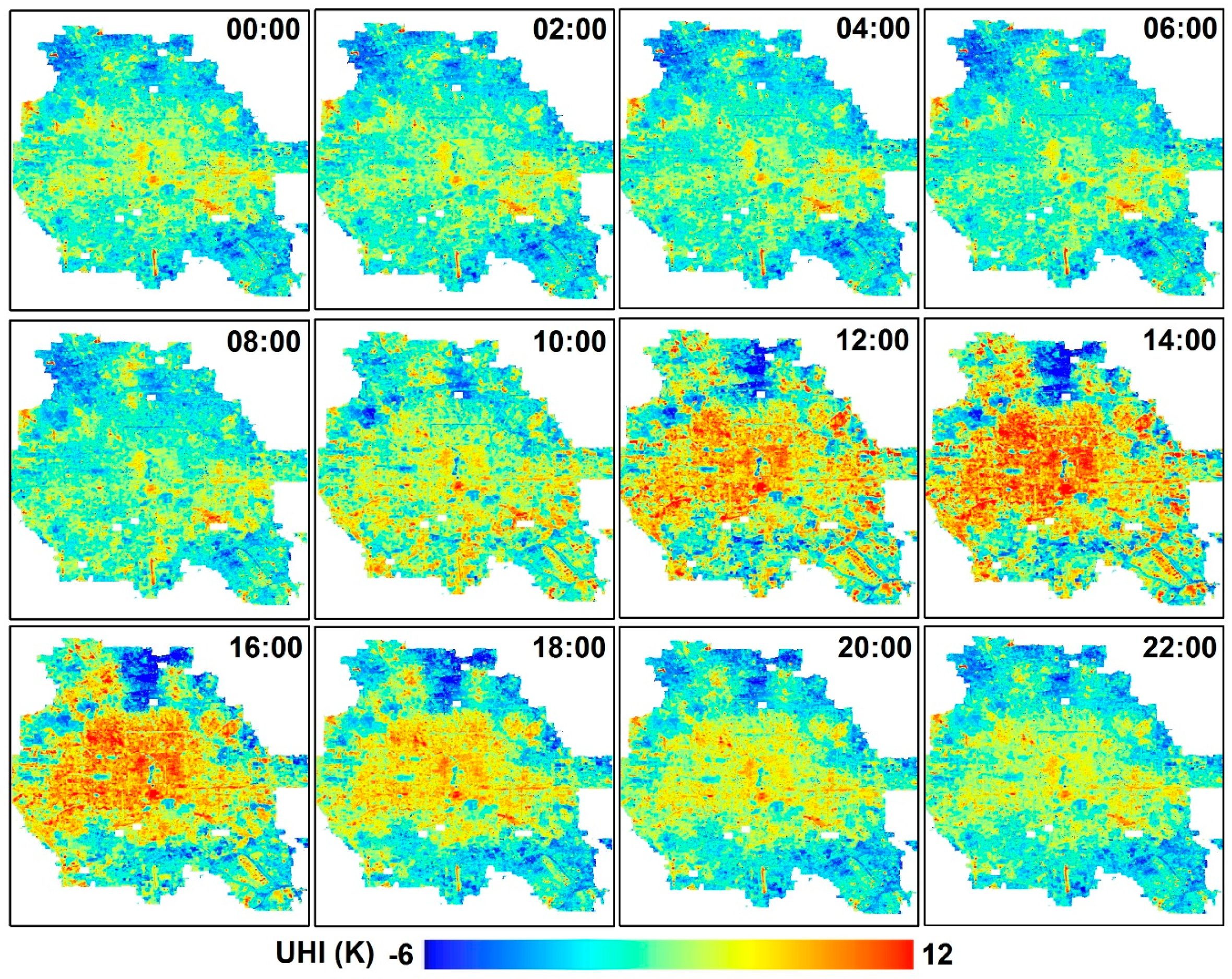
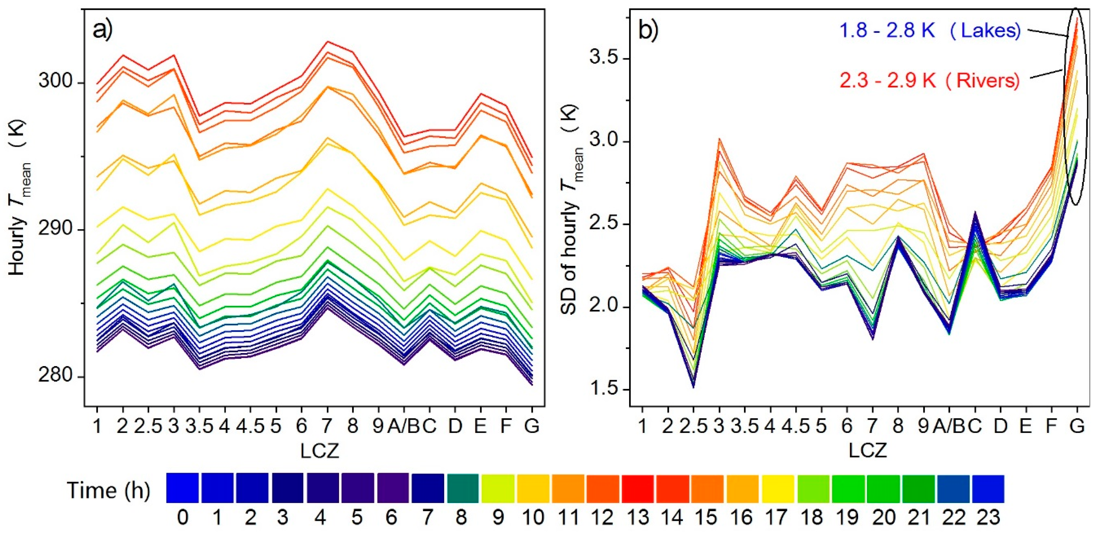
4.3. Diurnal Land Surface Temperature Variations
4.4. Frequencies of Heat Islands and Cool Islands at Multi-Temporal Scales
5. Discussion
5.1. Relationship between Land Surface Temperatures and Morphological and Coverage Indicators
5.2. Comparisons with Previous Studies
5.3. Implications for Public Health
6. Conclusions
Author Contributions
Funding
Acknowledgments
Conflicts of Interest
Appendix A

| LCZ | Indicators | LCZ | Indicators |
|---|---|---|---|
1 Compact high-rise | SVF: 0.2–0.4 BH(m): ≥25 BSF(%): 40–60 PSF%): <10 ISF(%): 40–60 | 8 Large low-rise | SVF: ≥0.7 BH(m): 3–10 BSF(%): 30–50 PSF(%): <20 ISF(%): 40–50 |
2 Compact mid-rise | SVF: 0.3–0.6 BH(m): 10–25 BSF(%): 40–70 PSF(%): <20 ISF(%): 30–50 | 9 Sparsely built | SVF: ≥0.8 BH(m): 3–10 BSF(%): 10–20 PSF(%): 60–80 ISF(%): <20 |
2.5 1 Extremely compact low-rise | BH(m): 4–10 BSF(%): ≥70 | 10 Heavy industry | SVF: 0.6–0.9 BH(m): 5–15 BSF(%): 20–30 PSF(%): 40–50 ISF(%): 20–40 |
3 Compact low-rise | SVF: 0.2–0.6 BH(m): 3–10 BSF(%): 40–70 PSF(%): <30 ISF(%): 20–50 | A Dense trees | SVF: <0.4 BH(m): 3–30 BSF(%): <10 PSF(%): ≥90 ISF(%): <10 |
3.5 1 Extremely open high-rise | BH(m): ≥25 BSF(%): 10–20 | B Scattered trees | SVF: 0.5–0.8 BH(m): 3–15 BSF(%): <10 PSF(%): ≥90 ISF(%): <10 |
4 Open high-rise | SVF: 0.5–0.7 BH(m): ≥25 BSF(%): 20–40 PSF(%): 30–40 ISF(%): 30–40 | C Bush, scrub | SVF: 0.7–0.8 BH(m): <2 BSF(%): <10 PSF(%): ≥90 ISF(%): <10 |
4.5 1 Extremely open mid-rise | BH(m): 10–25 BSF(%): 10–20 | D Low plants | SVF: ≥0.9 BH(m): <1 BSF(%): <10 PSF(%): ≥90 ISF(%): <10 |
5 Open mid-rise | SVF: 0.5–0.8 BH(m): 10–25 BSF(%): 20–40 PSF(%): 20–40 ISF(%): 30–50 | E Bare rock/paved | SVF: ≥0.9 BH(m): <0.25 BSF(%): <10 PSF(%): <10 ISF(%): ≥90 |
6 Open low-rise | SVF: 0.6–0.9 BH(m): 3–10 BSF(%): 20–40 PSF(%): 30–60 ISF(%): 20–50 | F Bare soil or sand | SVF: ≥0.9 BH(m): <0.25 BSF(%): <10 PSF(%): ≥90 ISF(%): <10 |
7 Lightweight low-rise | SVF: 0.2–0.5 BH(m): 2–4 BSF(%): 60–90 PSF(%): <30 ISF(%): <20 | G Water | SVF: ≥0.9 BH(m): - BSF(%): <10 PSF(%): ≥90 ISF(%): <10 |
Appendix B
Appendix C

Appendix D

References
- Oke, T.R. Boundary Layer Climates, 2nd ed.; Methuen: London, UK, 1987. [Google Scholar]
- Roth, M.; Oke, T.R.; Emery, W.J. Satellite-derived urban heat islands from three coastal cities and the utilization of such data in urban climatology. Int. J. Remote Sens. 1989, 10, 1699–1720. [Google Scholar] [CrossRef]
- Voogt, J.A.; Oke, T.R. Thermal remote sensing of urban climates. Remote Sens. Environ. 2003, 86, 370–384. [Google Scholar] [CrossRef]
- Quan, J.L.; Chen, Y.H.; Zhan, W.F.; Wang, J.F.; Voogt, J.; Wang, M.J. Multi-temporal trajectory of the urban heat island centroid in Beijing, China based on a Gaussian volume model. Remote Sens. Environ. 2014, 149, 33–46. [Google Scholar] [CrossRef]
- Zhou, D.; Xiao, J.; Bonafoni, S.; Berger, C.; Deilami, K.; Zhou, Y.; Frolking, S.; Yao, R.; Qiao, Z.; Sobrino, A.J.; et al. Satellite Remote Sensing of Surface Urban Heat Islands: Progress, Challenges, and Perspectives. Remote Sens. 2018, 11, 48. [Google Scholar] [CrossRef]
- Patz, J.A.; Campbell-Lendrum, D.; Holloway, T.; Foley, J.A. Impact of regional climate change on human health. Nature 2005, 438, 310–317. [Google Scholar] [CrossRef]
- Konopacki, S.; Akbari, H. Energy Savings for Heat-Island Reduction Strategies in Chicago and Houston (Including Updates for Baton Rouge, Sacramento, and Salt Lake City); Draft final report, LBNL-49638; University of California: Berkeley, CA, USA, 2002. [Google Scholar]
- Li, H.; Meier, F.; Lee, X.; Chakraborty, T.; Liu, J.; Schaap, M.; Sodoudi, S. Interaction between urban heat island and urban pollution island during summer in Berlin. Sci. Total Environ. 2018, 636, 818–828. [Google Scholar] [CrossRef]
- Peng, S.; Piao, S.; Ciais, P.; Friedlingstein, P.; Ottle, C.; Bréon, F.-M.; Nan, H.; Zhou, L.; Myneni, R.B. Surface urban heat island across 419 global big cities. Environ. Sci. Technol. 2012, 46, 696–703. [Google Scholar] [CrossRef]
- Zhou, D.C.; Zhao, S.Q.; Liu, S.G.; Zhang, L.X.; Zhu, C. Surface urban heat island in China’s 32 major cities: Spatial patterns and drivers. Remote Sens. Environ. 2014, 152, 51–61. [Google Scholar] [CrossRef]
- Arnfield, A.J. Two decades of urban climate research: A review of turbulence, exchanges of energy and water, and the urban heat island. Int. J. Climatol. 2003, 23, 1–26. [Google Scholar] [CrossRef]
- Stewart, I.D. A systematic review and scientific critique of methodology in modern urban heat island literature. Int. J. Climatol. 2011, 31, 200–217. [Google Scholar] [CrossRef]
- Stewart, I.D.; Oke, T.R. Local climate zones for urban temperature studies. Bull. Am. Meteorol. Soc. 2012, 93, 1879–1900. [Google Scholar] [CrossRef]
- Siu, L.W.; Hart, M.A. Quantifying urban heat island intensity in Hong Kong SAR, China. Environ. Monit. Assess. 2013, 185, 4383–4398. [Google Scholar] [CrossRef] [PubMed]
- Alexander, J.P.; Mills, G. Local climate classification and Dublin’s urban heat island. Atmosphere 2014, 5, 755–774. [Google Scholar] [CrossRef]
- Stewart, I.D.; Oke, T.R.; Krayenhoff, E.S. Evaluation of the local climate zone scheme using temperature observations and model simulations. Int. J. Climatol. 2014, 34, 1062–1080. [Google Scholar] [CrossRef]
- Leconte, F.; Bouyer, J.; Claverie, R.; Pétrissans, M. Using Local Climate Zone scheme for UHI assessment: Evaluation of the method using mobile measurements. Build. Environ. 2015, 83, 39–49. [Google Scholar] [CrossRef]
- Skarbit, N.; Stewart, I.D.; Unger, J.; Gál, T. Employing an urban meteorological network to monitor air temperature conditions in the ‘local climate zones’ of Szeged, Hungary. Int. J. Climatol. 2017, 37, 582–596. [Google Scholar] [CrossRef]
- Kotharkar, R.; Bagade, A. Evaluating urban heat island in the critical local climate zones of an Indian city. Landsc. Urban Plan. 2018, 169, 92–104. [Google Scholar] [CrossRef]
- Beck, C.; Straub, A.; Breitner, S.; Cyrys, J.; Philipp, A.; Rathmann, J.; Schneider, A.; Wolf, K.; Jacobeit, J. Air temperature characteristics of local climate zones in the Augsburg urban area (Bavaria, southern Germany) under varying synoptic conditions. Urban Clim. 2018, 25, 152–166. [Google Scholar] [CrossRef]
- Fenner, D.; Meier, F.; Bechtel, B.; Otto, M.; Scherer, D. Intra and inter ‘local climate zone’ variability of air temperature as observed by crowdsourced citizen weather stations in Berlin, Germany. Meteorol. Z. 2017, 26, 525–547. [Google Scholar] [CrossRef]
- Yang, X.; Yao, L.; Jin, T.; Peng, L.L.H.; Jiang, Z.; Hu, Z.; Ye, Y. Assessing the thermal behavior of different local climate zones in the Nanjing metropolis, China. Build. Environ. 2018, 137, 171–184. [Google Scholar] [CrossRef]
- Lindén, J.; Grimmond, C.S.B.; Esper, J. Urban warming in villages. Adv. Sci. Res. 2015, 12, 157–162. [Google Scholar] [CrossRef]
- Bokwa, A.; Hajto, M.J.; Walawender, J.P.; Szymanowski, M. Influence of diversified relief on the urban heat island in the city of Kraków, Poland. Theor. Appl. Climatol. 2015, 122, 365–382. [Google Scholar] [CrossRef]
- Geletič, J.; Lehnert, M.; Dobrovolný, P. Land surface temperature differences within local climate zones, based on two Central European cities. Remote Sens. 2016, 8, 788. [Google Scholar] [CrossRef]
- Chen, Y.; Quan, J.; Zhan, W.; Guo, Z. Enhanced statistical estimation of air temperature incorporating nighttime light data. Remote Sens. 2016, 8, 656. [Google Scholar] [CrossRef]
- Xiang, L.; Ren, C. Effects of the building typology on PET value in different local climate zones—A case study in Beijing, China. In Proceedings of the Passive and Low Energy Architecture (PLEA), Edinburgh, Scotland, 3–5 July 2017. [Google Scholar]
- Li, H.; Wolter, M.; Wang, X.; Sodoudi, S. Impact of land cover data on the simulation of urban heat island for Berlin using WRF coupled with bulk approach of Noah-LSM. Theor. Appl. Climatol. 2018, 134, 67–81. [Google Scholar] [CrossRef]
- Li, H.; Zhou, Y.; Wang, X.; Zhou, X.; Zhang, H.; Sodoudi, S. Quantifying urban heat island intensity and its physical mechanism using WRF/UCM. Sci. Total Environ. 2019, 650, 3110–3119. [Google Scholar] [CrossRef] [PubMed]
- Nassar, A.K.; Blackburn, G.A.; Whyatt, J.D. Dynamics and controls of urban heat sink and island phenomena in a desert city: Development of a local climate zone scheme using remotely-sensed inputs. Int. J. Appl. Earth Obs. Geoinf. 2016, 51, 76–90. [Google Scholar] [CrossRef]
- Cai, M.; Ren, C.; Xu, Y.; Lau, K.K.-L.; Wang, R. Investigating the relationship between local climate zone and land surface temperature using an improved WUDAPT methodology–A case study of Yangtze River Delta, China. Urban Clim. 2018, 24, 485–502. [Google Scholar] [CrossRef]
- Wang, R.; Cai, M.; Ren, C.; Bechtel, B.; Xu, Y.; Ng, E. Detecting multi-temporal land cover change and land surface temperature in Pearl River Delta by adopting local climate zone. Urban Clim. 2019, 28, 100455. [Google Scholar] [CrossRef]
- Wang, C.; Middel, A.; Myint, S.W.; Kaplan, S.; Brazel, A.J.; Lukasczyk, J. Assessing local climate zones in arid cities: The case of Phoenix, Arizona and Las Vegas, Nevada. ISPRS J. Photogramm. Remote Sens. 2018, 141, 59–71. [Google Scholar] [CrossRef]
- Schwarz, N.; Schlink, U.; Franck, U.; Großmann, K. Relationship of land surface and air temperatures and its implications for quantifying urban heat island indicators: An application for the city of Leipzig (Germany). Ecol. Indic. 2012, 18, 693–704. [Google Scholar] [CrossRef]
- Quan, J.L. Enhanced geographic information system-based mapping of local climate zones in Beijing, China. Sci. China Technol. Sci. 2019. [Google Scholar] [CrossRef]
- Yang, L.; Li, Y. City ventilation of Hong Kong at no-wind conditions. Atmos. Environ. 2009, 43, 3111–3121. [Google Scholar] [CrossRef]
- Quan, J.; Zhan, W.; Ma, T.; Du, Y.; Guo, Z.; Qin, B. An integrated model for generating hourly Landsat-like land surface temperatures over heterogeneous landscapes. Remote Sens. Environ. 2018, 206, 403–423. [Google Scholar] [CrossRef]
- Quan, J.L.; Zhan, W.F.; Chen, Y.H.; Wang, M.; Wang, J.F. Time series decomposition of remotely sensed land surface temperature and investigation of trends and seasonal variations in surface urban heat islands. J. Geophys. Res. Atmos. 2016, 121, 2638–2657. [Google Scholar] [CrossRef]
- Bechtel, B.; Alexander, J.P.; Böhner, J.; Ching, J.; Conrad, O.; Feddema, J.; Mills, G.; See, L.; Stewart, I. Mapping local climate zones for a worldwide database of the form and function of cities. ISPRS Int. J. Geo-Inf. 2015, 4, 199–219. [Google Scholar] [CrossRef]
- Mills, G.; Bechtel, B.; Ching, J.; See, L.; Feddema, J.; Foley, M.; Alexander, P.; O’Connor, M. An Introduction to the WUDAPT project. In Proceedings of the 9th International Conference on Urban Climates, Toulouse, France, 20–24 July 2015. [Google Scholar]
- Skarbit, N.; Gál, T.; Unger, J. Airborne surface temperature differences of the different Local Climate Zones in the urban area of a medium sized city. In Proceedings of the 2015 Joint Urban Remote Sensing Event (JURSE), Lausanne, Switzerland, 30 March–1 April 2015; pp. 1–4. [Google Scholar]
- Zhou, J.; Chen, Y.H.; Li, J.; Weng, Q.H.; Yi, W.B. A volume model for urban heat island based on remote sensing imagery and its application: A case study in Beijing. Int. J. Remote Sens. 2008, 12, 734–742. [Google Scholar]
- Wang, J.; Wang, K.; Wang, P. Urban heat (or cool) island over Beijing from MODIS land surface temperature. J. Remote Sens. 2007, 11, 330–339. [Google Scholar] [CrossRef]
- He, C.Y.; Chen, J.; Shi, P.J.; Fan, Y.D. City expansion model of metropolitan area in China: A case study of Beijing. Acta Geogr. Sin. 2003, 58, 294–304. [Google Scholar]
- Jiménez-Muñoz, J.C.; Sobrino, J.A.; Skoković, D.; Mattar, C.; Cristóbal, J. Land surface temperature retrieval methods from Landsat-8 thermal infrared sensor data. IEEE Geosci. Remote Sens. Lett. 2014, 11, 1840–1843. [Google Scholar] [CrossRef]
- Jimenez-Munoz, J.C.; Cristobal, J.; Sobrino, J.A.; Soria, G.; Ninyerola, M.; Pons, X.; Pons, X. Revision of the Single-Channel Algorithm for Land Surface Temperature Retrieval from Landsat Thermal-Infrared Data. IEEE Trans. Geosci. Remote Sens. 2009, 47, 339–349. [Google Scholar] [CrossRef]
- Wan, Z.M. New refinements and validation of the collection-6 MODIS land-surface temperature/emissivity product. Remote Sens. Environ. 2014, 140, 36–45. [Google Scholar] [CrossRef]
- Becker, F.; Li, Z. Surface temperature and emissivity at various scales: Definition, measurement and related problems. Remote Sens. Rev. 1995, 12, 225–253. [Google Scholar] [CrossRef]
- Agam, N.; Kustas, W.P.; Anderson, M.C.; Li, F.; Neale, C.M.U. A vegetation index based technique for spatial sharpening of thermal imagery. Remote Sens. Environ. 2007, 107, 545–558. [Google Scholar] [CrossRef]
- Kruskal, W.H.; Wallis, W.A. Use of ranks in one-criterion variance analysis. J. Am. Stat. Assoc. 1952, 47, 583–621. [Google Scholar] [CrossRef]
- Bechtel, B. Multitemporal Landsat data for urban heat island assessment and classification of local climate zones. In Proceedings of the 2011 Joint Urban Remote Sensing Event (JURSE), Munich, Germany, 11–13 April 2011. [Google Scholar]
- Huang, F.; Zhan, W.; Voogt, J.; Hu, L.; Wang, Z.; Quan, J.; Ju, W.; Guo, Z. Temporal upscaling of surface urban heat island by incorporating an annual temperature cycle model: A tale of two cities. Remote Sens. Environ. 2016, 186, 1–12. [Google Scholar] [CrossRef]
- Krayenhoff, S.E.; Voogt, A.J. Daytime thermal anisotropy of urban neighbourhoods: Morphological causation. Remote Sens. 2016, 8, 108. [Google Scholar] [CrossRef]
- Vinnikov, K.Y.; Yu, Y.; Goldberg, M.D.; Tarpley, D.; Romanov, P.; Laszlo, I.; Chen, M. Angular anisotropy of satellite observations of land surface temperature. Geophys. Res. Lett. 2012, 39, L23802. [Google Scholar] [CrossRef]
- Yang, X.; Li, Y.; Luo, Z.; Chan, P.W. The urban cool island phenomenon in a high-rise high-density city and its mechanisms. Int. J. Climatol. 2017, 37, 890–904. [Google Scholar] [CrossRef]
- Lai, J.; Zhan, W.; Huang, F.; Voogt, J.; Bechtel, B.; Allen, M.; Peng, S.; Hong, F.; Liu, Y.; Du, P.; et al. Identification of typical diurnal patterns for clear-sky climatology of surface urban heat islands. Remote Sens. Environ. 2018, 217, 203–220. [Google Scholar] [CrossRef]
- Zhou, J.; Chen, Y.H.; Zhang, X.; Zhan, W.F. Modeling the diurnal variations of urban heat islands with multi-source satellite data. Int. J. Remote Sens. 2013, 34, 7568–7588. [Google Scholar] [CrossRef]
- Kalnay, E.; Cai, M. Impact of urbanization and land-use change on climate. Nature 2003, 423, 528–531. [Google Scholar] [CrossRef] [PubMed]
- Zhan, W.F.; Chen, Y.H.; Zhou, J.; Li, J. Spatial simulation of urban heat island intensity based on the Support Vector Machine technique: A case study in Beijing. Acta Geodaetica et Cartographica Sinica 2011, 40, 96–103. [Google Scholar]
- Berger, C.; Rosentreter, J.; Voltersen, M.; Baumgart, C.; Schmullius, C.; Hese, S. Spatio-temporal analysis of the relationship between 2D/3D urban site characteristics and land surface temperature. Remote Sens. Environ. 2017, 193, 225–243. [Google Scholar] [CrossRef]
- Yuan, F.; Bauer, M.E. Comparison of impervious surface area and normalized difference vegetation index as indicators of surface urban heat island effects in Landsat imagery. Remote Sens. Environ. 2007, 106, 375–386. [Google Scholar] [CrossRef]
- Hauke, J.; Kossowski, T. Comparison of values of Pearson’s and Spearman’s correlation coefficients on the same sets of data. Quaest. Geogr. 2011, 30, 87–93. [Google Scholar] [CrossRef]
- Kato, S.; Matsunaga, T.; Yamaguchi, Y. Influence of Shade on Surface Temperature in an Urban Area Estimated by ASTER Data. In Proceedings of the International Archives of the Photogammetry, Remote Sensing and Spatial Information Science, Kyoto, Japan, 12–14 March 2019; pp. 925–929. [Google Scholar]
- Middel, A.; Häb, K.; Brazel, A.J.; Martin, C.A.; Guhathakurta, S. Impact of urban form and design on mid-afternoon microclimate in Phoenix Local Climate Zones. Landsc. Urban Plan. 2014, 122, 16–28. [Google Scholar] [CrossRef]
- Cai, H.; Xu, X. Impacts of built-up area expansion in 2D and 3D on regional surface temperature. Sustainability 2017, 9, 1862. [Google Scholar] [CrossRef]
- Huang, X.; Wang, Y. Investigating the effects of 3D urban morphology on the surface urban heat island effect in urban functional zones by using high-resolution remote sensing data: A case study of Wuhan, Central China. ISPRS J. Photogramm. Remote Sens. 2019, 152, 119–131. [Google Scholar] [CrossRef]
- Ma, Q.; Wu, J.; He, C. A hierarchical analysis of the relationship between urban impervious surfaces and land surface temperatures: Spatial scale dependence, temporal variations, and bioclimatic modulation. Landsc. Ecol. 2016, 31, 1139–1153. [Google Scholar] [CrossRef]
- Dousset, B.; Gourmelon, F.; Laaidi, K.; Zeghnoun, A.; Giraudet, E.; Bretin, P.; Mauri, E.; Vandentorren, S. Satellite monitoring of summer heat waves in the Paris metropolitan area. Int. J. Climatol. 2011, 31, 313–323. [Google Scholar] [CrossRef]
- Oke, T.R. The energetic basis of the urban heat island. Q. J. R. Meteorol. Soc. 1982, 108, 1–24. [Google Scholar] [CrossRef]
- van Hove, L.W.A.; Jacobs, C.M.J.; Heusinkveld, B.G.; Elbers, J.A.; van Driel, B.L.; Holtslag, A.A.M. Temporal and spatial variability of urban heat island and thermal comfort within the Rotterdam agglomeration. Build. Environ. 2015, 83, 91–103. [Google Scholar] [CrossRef]
- Weng, Q.H.; Rajasekar, U.; Hu, X.F. Modeling urban heat islands and their relationship with impervious surface and vegetation abundance by using ASTER images. IEEE Trans. Geosci. Remote Sens. 2011, 49, 4080–4089. [Google Scholar] [CrossRef]
- Weng, Q.H.; Hu, X.F.; Liu, H. Estimating impervious surfaces using linear spectral mixture analysis with multitemporal ASTER images. Int. J. Remote Sens. 2009, 30, 4807–4830. [Google Scholar] [CrossRef]
- Lu, D.S.; Weng, Q.H. Spectral mixture analysis of ASTER images for examining the relationship between urban thermal features and biophysical descriptors in Indianapolis, Indiana, USA. Remote Sens. Environ. 2006, 104, 157–167. [Google Scholar] [CrossRef]
- Schwarz, N.; Manceur Ameur, M. Analyzing the Influence of Urban Forms on Surface Urban Heat Islands in Europe. J. Urban Plan. Dev. 2015, 141, A4014003. [Google Scholar] [CrossRef]
- Steeneveld, G.J.; Koopmans, S.; Heusinkveld, B.G.; Theeuwes, N.E. Refreshing the role of open water surfaces on mitigating the maximum urban heat island effect. Landsc. Urban Plan. 2014, 121, 92–96. [Google Scholar] [CrossRef]
- Morris, C.J.G.; Simmonds, I.; Plummer, N. Quantification of the influences of wind and cloud on the nocturnal urban heat island of a large city. J. Appl. Meteorol. 2001, 40, 169–182. [Google Scholar] [CrossRef]
- Lelovics, E.; Unger, J.; Gál, T.; Gál, C.V. Design of an urban monitoring network based on Local Climate Zone mapping and temperature pattern modelling. Clim. Res. 2014, 60, 51–62. [Google Scholar] [CrossRef]
- Stoll, M.J.; Brazel, A.J. Surface-air temperature relationships in the urban environment of Phoenix, Arizona. Phys. Geogr. 1992, 13, 160–179. [Google Scholar] [CrossRef]
- Dousset, B.; Gourmelon, F. Satellite multi-sensor data analysis of urban surface temperatures and landcover. ISPRS J. Photogramm. Remote Sens. 2003, 58, 43–54. [Google Scholar] [CrossRef]
- Zhao, S.; Liu, S.; Zhou, D. Prevalent vegetation growth enhancement in urban environment. Proc. Natl. Acad. Sci. USA 2016, 113, 6313. [Google Scholar] [CrossRef] [PubMed]
- Zhou, D.; Zhao, S.; Zhang, L.; Liu, S. Remotely sensed assessment of urbanization effects on vegetation phenology in China’s 32 major cities. Remote Sens. Environ. 2016, 176, 272–281. [Google Scholar] [CrossRef]
- Grimm, N.B.; Faeth, S.H.; Golubiewski, N.E.; Redman, C.L.; Wu, J.; Bai, X.; Briggs, J.M. Global Change and the Ecology of Cities. Science 2008, 319, 756–760. [Google Scholar] [CrossRef] [PubMed]
- Liu, X.; Liu, H.; Fan, H.; Liu, Y.; Ding, G. Influence of Heat Waves on Daily Hospital Visits for Mental Illness in Jinan, China—A Case-Crossover Study. Int. J. Environ. Res. Public Health 2018, 16, 87. [Google Scholar] [CrossRef] [PubMed]
- Chirico, F.; Magnavita, N. New and Old Indices for Evaluating Heat Stress in an Indoor Environment: Some Considerations. Comment on Kownacki, L.; Gao, C.; Kuklane, K.; Wierzbicka, A. Heat Stress in Indoor Environments of Scandinavian Urban Areas: A Literature Review. Int. J. Environ. Res. Public Health 2019, 16, 1444. [Google Scholar] [CrossRef]
- Liu, H.; Weng, Q. Enhancing temporal resolution of satellite imagery for public health studies: A case study of West Nile Virus outbreak in Los Angeles in 2007. Remote Sens. Environ. 2012, 117, 57–71. [Google Scholar] [CrossRef]
- Xue, T.; Zhu, T.; Zheng, Y.; Zhang, Q. Declines in mental health associated with air pollution and temperature variability in China. Nat. Commun. 2019, 10. [Google Scholar] [CrossRef]
- Lo, C.P.; Quattrochi, D.A. Land-Use and Land-Cover Change, Urban Heat Island Phenomenon, and Health Implications. Photogramm. Eng. Remote Sens. 2003, 69, 1053–1063. [Google Scholar] [CrossRef]
- Zanobetti, A.; Schwartz, J. Temperature and mortality in nine US cities. Epidemiology 2008, 19, 563–570. [Google Scholar] [CrossRef] [PubMed]
- Mironova, V.; Shartova, N.; Beljaev, A.; Varentsov, M.; Grishchenko, M. Effects of Climate Change and Heterogeneity of Local Climates on the Development of Malaria Parasite (Plasmodium vivax) in Moscow Megacity Region. Int. J. Environ. Res. Public Health 2019, 16, 694. [Google Scholar] [CrossRef] [PubMed]
- Verdonck, M.-L.; Demuzere, M.; Hooyberghs, H.; Beck, C.; Cyrys, J.; Schneider, A.; Dewulf, R.; Van Coillie, F. The potential of local climate zones maps as a heat stress assessment tool, supported by simulated air temperature data. Landsc. Urban Plan. 2018, 178, 183–197. [Google Scholar] [CrossRef]
- Geletič, J.; Lehnert, M.; Savić, S.; Milošević, D. Modelled spatiotemporal variability of outdoor thermal comfort in local climate zones of the city of Brno, Czech Republic. Sci. Total Environ. 2018, 624, 385–395. [Google Scholar] [CrossRef] [PubMed]
- Lau, K.K.-L.; Chung, S.C.; Ren, C. Outdoor thermal comfort in different urban settings of sub-tropical high-density cities: An approach of adopting local climate zone (LCZ) classification. Build. Environ. 2019, 154, 227–238. [Google Scholar] [CrossRef]
- Lundgren Kownacki, K.; Gao, C.; Kuklane, K.; Wierzbicka, A. Heat Stress in Indoor Environments of Scandinavian Urban Areas: A Literature Review. Int. J. Environ. Res. Public Health 2019, 16, 560. [Google Scholar] [CrossRef] [PubMed]
- Franck, U.; Krüger, M.; Schwarz, N.; Grossmann, K.; Röder, S.; Schlink, U. Heat stress in urban areas: Indoor and outdoor temperatures in different urban structure types and subjectively reported well-being during a heat wave in the city of Leipzig. Meteorol. Z. 2013, 22, 167–177. [Google Scholar] [CrossRef]
- Quinn, A.; Tamerius, J.D.; Perzanowski, M.; Jacobson, J.S.; Goldstein, I.; Acosta, L.; Shaman, J. Predicting indoor heat exposure risk during extreme heat events. Sci. Total Environ. 2014, 490, 686–693. [Google Scholar] [CrossRef] [PubMed]
- Xu, Y.; Qin, Z.H.; Wan, H. Advances in the study of near surface air temperature retrieval from thermal infrared remote sensing. Remote Sens. Land Resour. 2011, 23, 9–14. [Google Scholar]
- Chen, F.; Liu, Y.; Liu, Q.; Qin, F. A statistical method based on remote sensing for the estimation of air temperature in China. Int. J. Climatol. 2015, 35, 2131–2143. [Google Scholar] [CrossRef]
- Kloog, I.; Chudnovsky, A.; Koutrakis, P.; Schwartz, J. Temporal and spatial assessments of minimum air temperature using satellite surface temperature measurements in Massachusetts, USA. Sci. Total Environ. 2012, 432, 85–92. [Google Scholar] [CrossRef] [PubMed]
- Ho, H.C.; Knudby, A.; Sirovyak, P.; Xu, Y.; Hodul, M.; Henderson, S.B. Mapping maximum urban air temperature on hot summer days. Remote Sens. Environ. 2014, 154, 38–45. [Google Scholar] [CrossRef]
- Ceccato, P.; Vancutsem, C.; Temimi, M. Monitoring air and Land Surface Temperatures from remotely sensed data for climate-human health applications. In Proceedings of the 2010 IEEE International Geoscience and Remote Sensing Symposium (IGARSS), Honolulu, HI, USA, 25–30 July 2010; pp. 178–180. [Google Scholar]
- Tomlinson, C.J.; Chapman, L.; Thornes, J.E.; Baker, C.J. Including the urban heat island in spatial heat health risk assessment strategies: A case study for Birmingham, UK. Int. J. Health Geogr. 2011, 10, 42. [Google Scholar] [CrossRef] [PubMed]
- Dong, W.; Liu, Z.; Zhang, L.; Tang, Q.; Liao, H.; Li, X. Assessing Heat Health Risk for Sustainability in Beijing’s Urban Heat Island. Sustainability 2014, 6, 7334–7357. [Google Scholar] [CrossRef]
- White-Newsome, J.L.; Brines, S.J.; Brown, D.G.; Dvonch, J.T.; Gronlund, C.J.; Zhang, K.; Oswald, E.M.; O’Neill, M.S. Validating Satellite-Derived Land Surface Temperature with in Situ Measurements: A Public Health Perspective. Environ. Health Perspect. 2013, 121, 925–931. [Google Scholar] [CrossRef] [PubMed]
- Zhu, W.; Lq, A.; Jia, S. Estimation of daily maximum and minimum air temperature using MODIS land surface temperature products. Remote Sens. Environ. 2013, 130, 62–73. [Google Scholar] [CrossRef]
- Basu, R. High ambient temperature and mortality: A review of epidemiologic studies from 2001 to 2008. Environ. Health 2009, 8, 40. [Google Scholar] [CrossRef]
- Shen, H.; Huang, L.; Zhang, L.; Wu, P.; Zeng, C. Long-term and fine-scale satellite monitoring of the urban heat island effect by the fusion of multi-temporal and multi-sensor remote sensed data: A 26-year case study of the city of Wuhan in China. Remote Sens. Environ. 2016, 172, 109–125. [Google Scholar] [CrossRef]


| Data | Observation Time (YYYY/MM/DD) | Spatial Resolution (m) | Layer/Band/Class |
|---|---|---|---|
| City street map (CSM) | 2016/03 | Vector→15 | Block, building, street, water, green space |
| Landsat-8 OLI 1 | 2016/05/04 | 15 | Red and near infrared bands |
| Land cover map | 2017 | 30 | Forest, shrubland, cropland, grassland, impervious land, bare land, water, snow/ice |
| Date (YYYY/MM/DD) | Landsat-8 TIRS 1 | MODIS 2 | FY-2F 3 (h) | Date (YYYY/MM/DD) | Landsat-8 TIRS | MODIS | FY-2F (h) |
|---|---|---|---|---|---|---|---|
| Observation Time (hh:mm) | Observation Time (hh:mm) | ||||||
| 2017/07/10 | 10:54 | 10:48 | 2018/01/11 | - | 11:39,12:33,22:00,01:33 | 24 | |
| 2017/07/11 | - | 10:49,13:28,22:54,02:08 | 24 | 2018/01/13 | - | 11:30,12:27,21:54,02:47 | 24 |
| 2017/09/07 | - | 11:30,12:28,21:54,02:45 | 24 | 2018/02/03 | 10:54 | 11:10 | |
| 2017/09/12 | 10:54 | 11:10 | 2018/02/05 | - | 11:32,12:30,21:58,02:51 | 24 | |
| 2017/09/18 | - | 11:08,13:39,21:34,02:25 | 24 | 2018/02/12 | - | 11:39,12:33,22:00,01:19 | 24 |
| 2017/09/20 | - | 10:59,13:30,21:20,02:13 | 24 | 2018/02/16 | - | 11:17,12:16,21:35,02:34 | 24 |
| 2017/09/28 | 10:54 | 11:00 | 2018/03/02 | - | 11:30,12:27,21:54,02:44 | 24 | |
| 2017/09/29 | - | 10:51,13:28,22:39,02:08 | 24 | 2018/03/25 | - | 11:33,12:30,21:58,02:52 | 24 |
| 2017/10/05 | - | 10:42,12:50,22:08,01:30 | 24 | 2018/04/08 | 10:54 | 10:50 | |
| 2017/10/24 | - | 10:45,13:20,22:49,02:00 | 24 | 2018/04/11 | - | 10:36,13:10,22:39,01:57 | 24 |
| 2017/10/30 | 10:54 | 11:49,12:40,22:02,01:24 | 24 | 2018/04/16 | - | 11:00,13:30,21:20,02:17 | 24 |
| 2017/11/04 | - | 10:27,13:00,22:23,01:42 | 24 | 2018/04/27 | - | 10:37,13:10,22:39,01:57 | 24 |
| 2017/11/08 | - | 11:42,12:33,22:00,01:20 | 24 | 2018/05/23 | - | 11:19,13:41,21:38,02:34 | 24 |
| 2017/11/11 | - | 10:31,13:03,22:27,01:48 | 24 | 2018/05/28 | - | 11:33,12:30,21:59,02:37 | 24 |
| 2017/11/15 | 10:54 | 10:51 | 2018/05/31 | - | 10:30,13:00,22:25,01:43 | 24 | |
| 2017/12/01 | 10:54 | 11:45,12:40,22:02,01:24 | 24 | 2018/06/20 | - | 11:41,12:33,22:01,01:20 | 24 |
| 2017/12/17 | 10:54 | 11:48,12:40,22:02,01:24 | 24 | 2018/06/27 | 10:54 | 11:36,12:43,22:06,01:24 | 24 |
| 2017/12/21 | - | 11:23,12:23,21:40,02:38 | 24 | ||||
| Spatial resolution (m) | Source | ||||||
| 100 | 1000 | 5000 | USGS 4 | EOSDIS 5 | NSMC 6 | ||
| Parameter | Definition and Calculation |
|---|---|
| Daily/daytime/nighttime | Average of LSTs during a day/08:00–16:00/20:00–04:00 |
| Annual/monthly | Average of daily in one year/month |
| Hourly | Average of LSTs at a certain hour in one year |
| Annual temperature range (ATR) | Difference between the maximum and minimum daily in one year |
| Daily / | Maximum/minimum LST during 24 hours |
| Daily / | Time when daily / occurs |
| Diurnal temperature range (DTR) | Difference between daily and |
| Heat/cool island frequency (HIF/CIF) | Rate at which a heat/cool island with a certain intensity occurs during the year/season/daytime/nighttime |
| Parameter | SVF 2 | BH 3 | BSF 4 | VSF 5 | ISF 6 |
|---|---|---|---|---|---|
| Annual | −0.12 | −0.26 (+0.16) | +0.24 | −0.32 | +0.03 (+0.32) |
| Annual temperature range (ATR) | −0.41 | +0.10 (+0.31) | +0.32 | −0.52 | +0.03 (+0.40) |
| Summer daytime | −0.40 | −0.13 (+0.35) | +0.41 | −0.49 | +0.01 (+0.49) |
| Winter daytime | +0.19 | −0.33 (−0.08) | +0.01 | +0.21 | +0.00 (+0.03) |
| Summer nighttime | −0.29 | −0.09 (+0.27) | +0.31 | −0.35 | −0.00 (+0.36) |
| Winter nighttime | +0.16 | −0.27 (−0.06) | +0.01 | +0.19 | −0.01 (+0.01) |
| Summer diurnal temperature range (DTR) | −0.29 | −0.03 (+0.24) | +0.27 | −0.37 | +0.02 (+0.36) |
| Winter DTR | +0.08 | +0.00 (−0.07) | −0.06 | +0.02 | +0.07 (+0.03) |
| Annual heat island frequency (HIF) | −0.18 | −0.25 (+0.20) | +0.27 | −0.32 | +0.02 (+0.32) |
| Annual cool island frequency (CIF) | +0.14 | +0.24 (−0.16) | −0.22 | +0.26 | −0.03 (−0.26) |
| Category | Remotely Sensed LST-Based Studies | In situ air Temperature (AT)-Based Studies | ||||||||||||||
|---|---|---|---|---|---|---|---|---|---|---|---|---|---|---|---|---|
| Source/Reference | This Study | [41] | [25] | [31] | [31] | [33] | [33] | [15] | [16] | [17] | [18] | [22] | ||||
| Study area | City Country | Beijing China | Szeged Hungary | Prague and Brno Czech Republic | Shanghai China | Hangzhou China | Phoenix USA | Las Vegas USA | Dublin Ireland | Vancouver Canada | Nancy France | Szeged Hungary | Nanjing China | |||
| Latitude Longitude | 40°N 116°E | 46°N 20°E | 50°N and 49°N 14°E and 16°E | 30°N 121°E | 29°N 119°E | 33°N 112°W | 36°N 115°W | 54°N 7°E | 49°N 123°E | 49°N 6°E | 46°N 20°E | 32°N 119°E | ||||
| Population (million) | 22 | 0.16 | 1.3 and 0.4 | 24 | 9.8 | 1.5 | 0.5 | 1.2 | 2 | 0.3 | 0.16 | 8.3 | ||||
| Data | Acquisition method | Landsat, MODIS 1 and FY 2 fusion | Airborne thermal camera | Landsat and ASTER 3 | ASTER | ASTER | ASTER | ASTER | Fixed sites and mobile | Mobile | Mobile | Fixed sites | Fixed sites | |||
| Time period (number of days) | 1 year, hourly (29) | Summer night (2) | Spring, summer and autumn day (8 for each city) | Summer and autumn night (2) | Summer and autumn night (2) | Spring day and night (2) | Spring day and summer night (2) | Summer (3) | Spring (4) | Summer (9–17) | 1 year (32) | >1 year (78) | ||||
| Result | Number of LCZs (sub-/supplementary class) | 18 (3) | 7 (0) | 15 (0) | 17 (0) | 17 (0) | 14 (0) | 14 (0) | 4 (0) | 8 (1) | 5 (0) | 7 (0) | 14 (6) | |||
| Annual/seasonal pattern | Y | N | Y | N | N | N | N | N | N | N | Y | Y | ||||
| Diurnal pattern | Y (diurnal parameter) | N | N | N | N | Y (day-night) | Y (day-night) | N | Y (DTR 4) | Y (day-night) | Y | Y | ||||
| Period of statistics | Annual | Night | Day | Night | Night | Day | Night | Day | Night | Night | Night | Night | Day | Day | Night | |
| LCZ 1 | x | x | H3 | H2 | x | x | x | x | x | H1 | x | x | x | x | ||
| LCZ 2 | H3 | H1 | H3 | x | x | x | x | H1 | x | H1 | H1 | H3 | H2 | |||
| LCZ 3 | H4 | H3 | H2 | x | x | x | x | H2 | x | x | H1 | x | x | |||
| LCZ 4 | x | H4 | H2 | H2 | x | H2 | x | x | C4 | H4 | ||||||
| LCZ 5 | H4 | H3 | x | x | H2 | H2 | H4 | C3 | ||||||||
| LCZ 6 | C3 | H3 | C4 | H4 | H4 | x | x | |||||||||
| LCZ 7 | H1 | x | x | H1 | x | x | x | x | x | x | ||||||
| LCZ 8 | H2 | H2 | H4 | H2 | H3 | H2 | H1 | x | H3 | H3 | H3 | H1 | x | |||
| LCZ 9 | C2 | C1 | C2 | x | H4 | x | C2 | C1 | ||||||||
| LCZ 10 | x | x | H1 | H4 | H3 | H4 | H4 | x | x | x | x | H2 | H1 | |||
| LCZ A | C2 | C1 | C2 | C2 | C2 | C4 | C3 | C4 | x | C2 | x | x | C1 | C3 | ||
| LCZ B | x | C3 | C3 | C3 | C1 | x | C3 | x | x | C3 | ||||||
| LCZ C | C3 | x | C4 | C1 | C4 | H4 | H3 | C3 | x | x | x | x | x | x | ||
| LCZ D | C4 | x | C3 | C2 | C1 | C2 | C2 | C1 | C1 | C1 | C1 | C3 | C2 | |||
| LCZ E | x | H2 | H1 | H1 | x | x | x | x | x | x | ||||||
| LCZ F | x | C4 | C3 | H3 | H4 | C4 | x | x | x | x | x | x | ||||
| LCZ G | C1 | x | C1 | H1 | H1 | C1 | C4 | C1 | x | x | x | x | C2 | H3 | ||
© 2019 by the author. Licensee MDPI, Basel, Switzerland. This article is an open access article distributed under the terms and conditions of the Creative Commons Attribution (CC BY) license (http://creativecommons.org/licenses/by/4.0/).
Share and Cite
Quan, J. Multi-Temporal Effects of Urban Forms and Functions on Urban Heat Islands Based on Local Climate Zone Classification. Int. J. Environ. Res. Public Health 2019, 16, 2140. https://doi.org/10.3390/ijerph16122140
Quan J. Multi-Temporal Effects of Urban Forms and Functions on Urban Heat Islands Based on Local Climate Zone Classification. International Journal of Environmental Research and Public Health. 2019; 16(12):2140. https://doi.org/10.3390/ijerph16122140
Chicago/Turabian StyleQuan, Jinling. 2019. "Multi-Temporal Effects of Urban Forms and Functions on Urban Heat Islands Based on Local Climate Zone Classification" International Journal of Environmental Research and Public Health 16, no. 12: 2140. https://doi.org/10.3390/ijerph16122140
APA StyleQuan, J. (2019). Multi-Temporal Effects of Urban Forms and Functions on Urban Heat Islands Based on Local Climate Zone Classification. International Journal of Environmental Research and Public Health, 16(12), 2140. https://doi.org/10.3390/ijerph16122140