Direct Prediction of the Toxic Gas Diffusion Rule in a Real Environment Based on LSTM


Abstract
:1. Introduction
2. Theories
2.1. Brief Description of Dataset
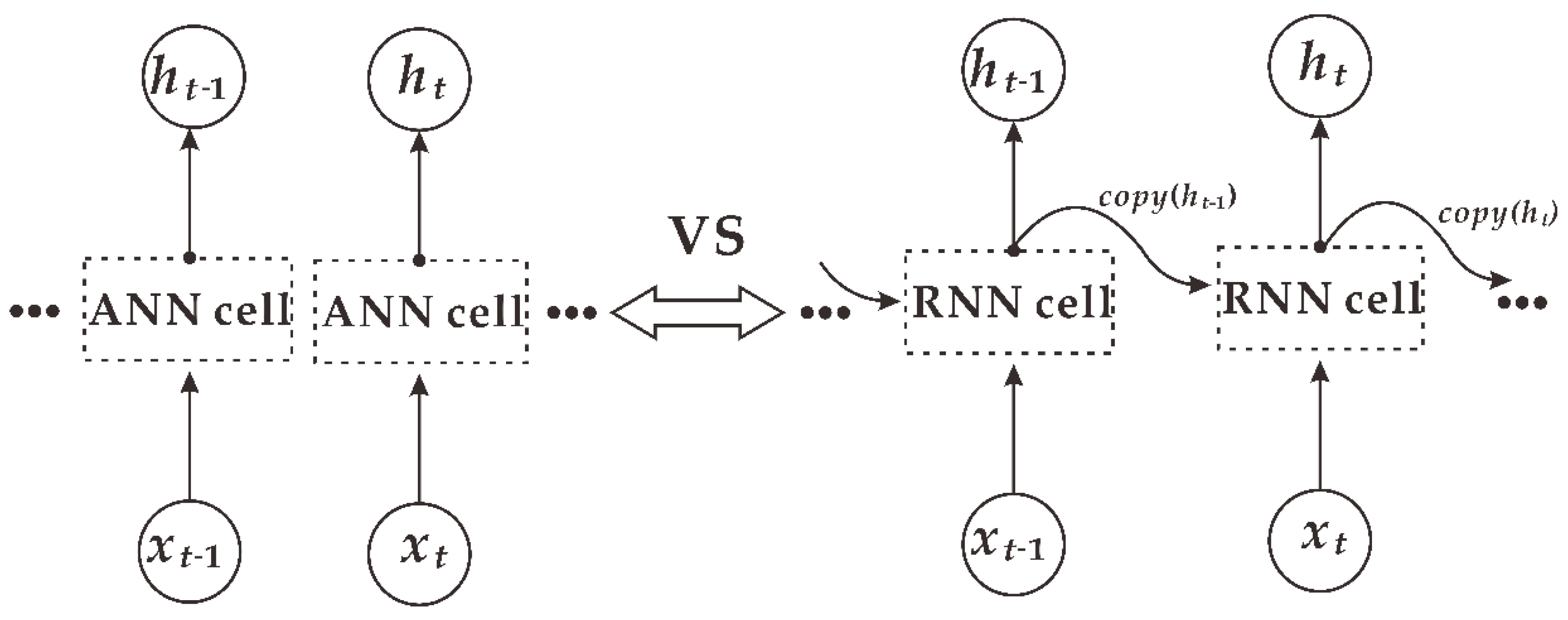
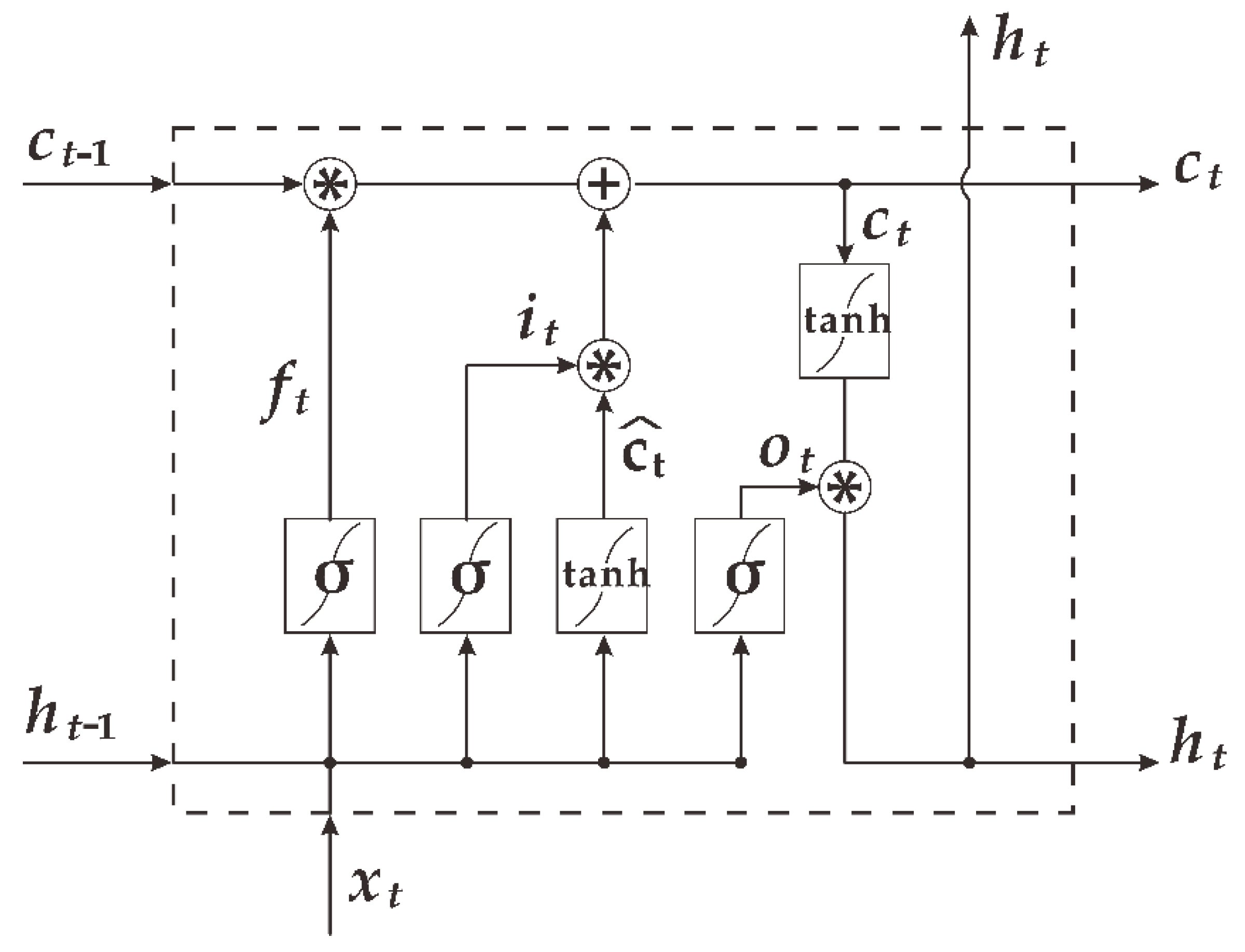
2.2. The Long Short-Term Memory Network
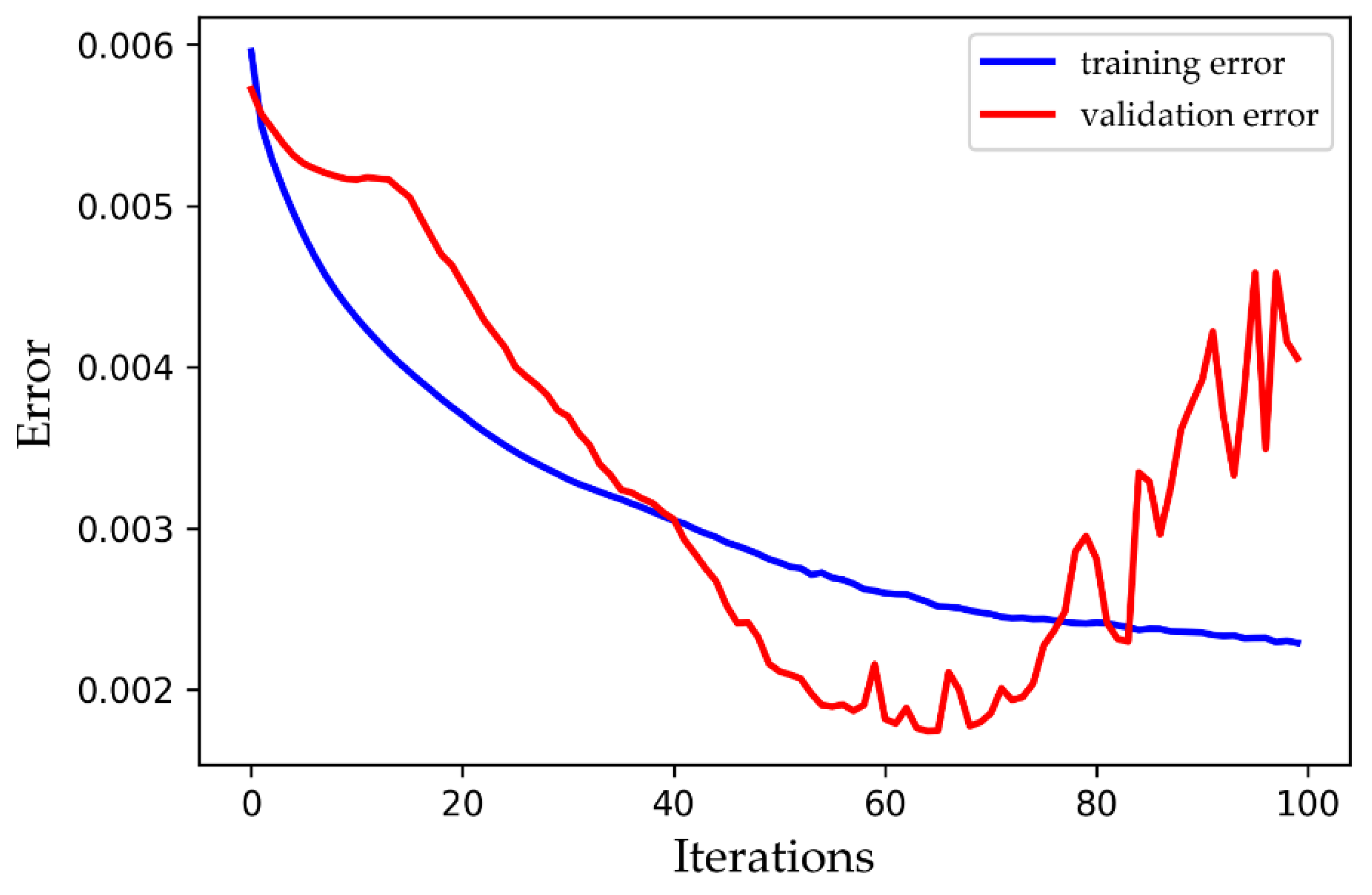
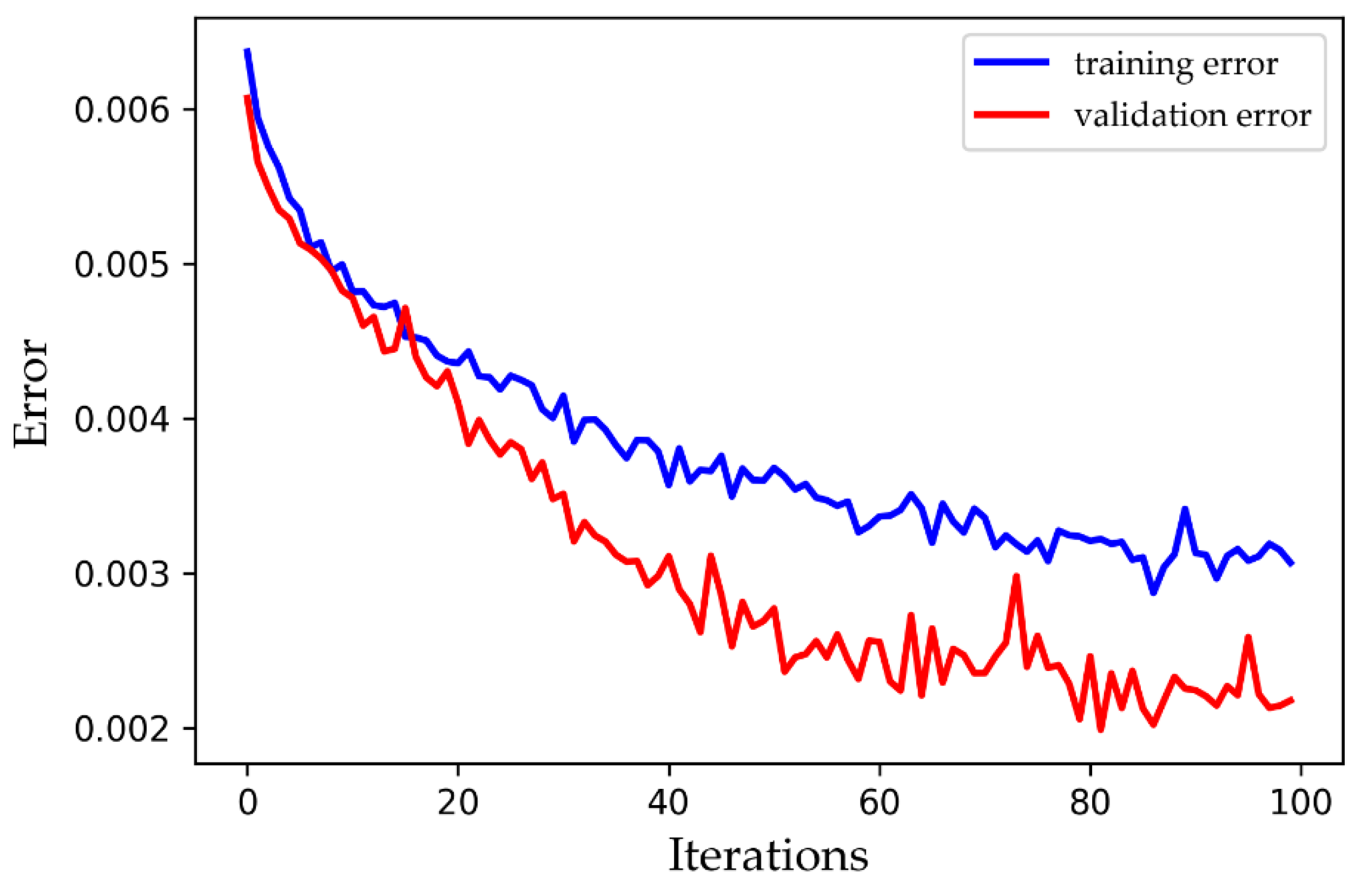
2.3. Overfitting
3. Methods
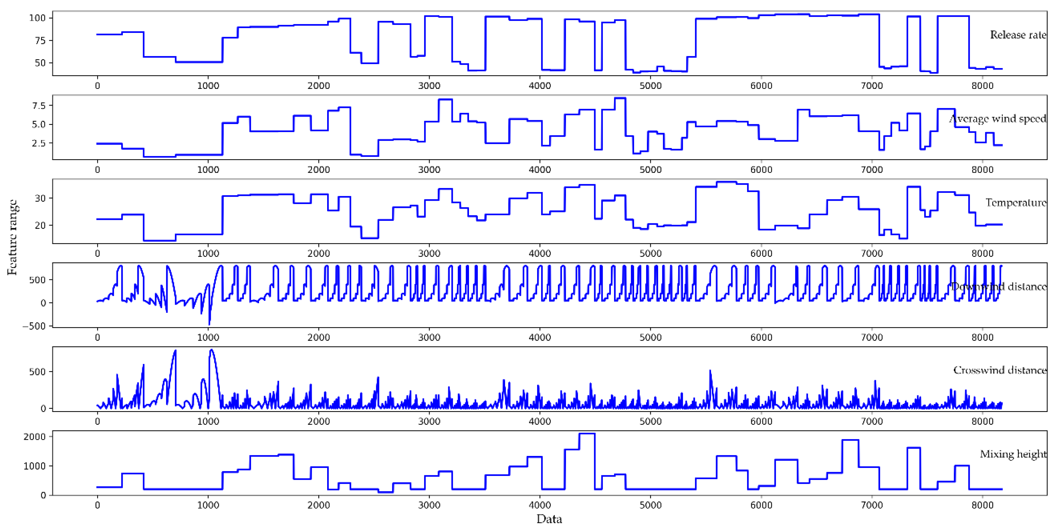
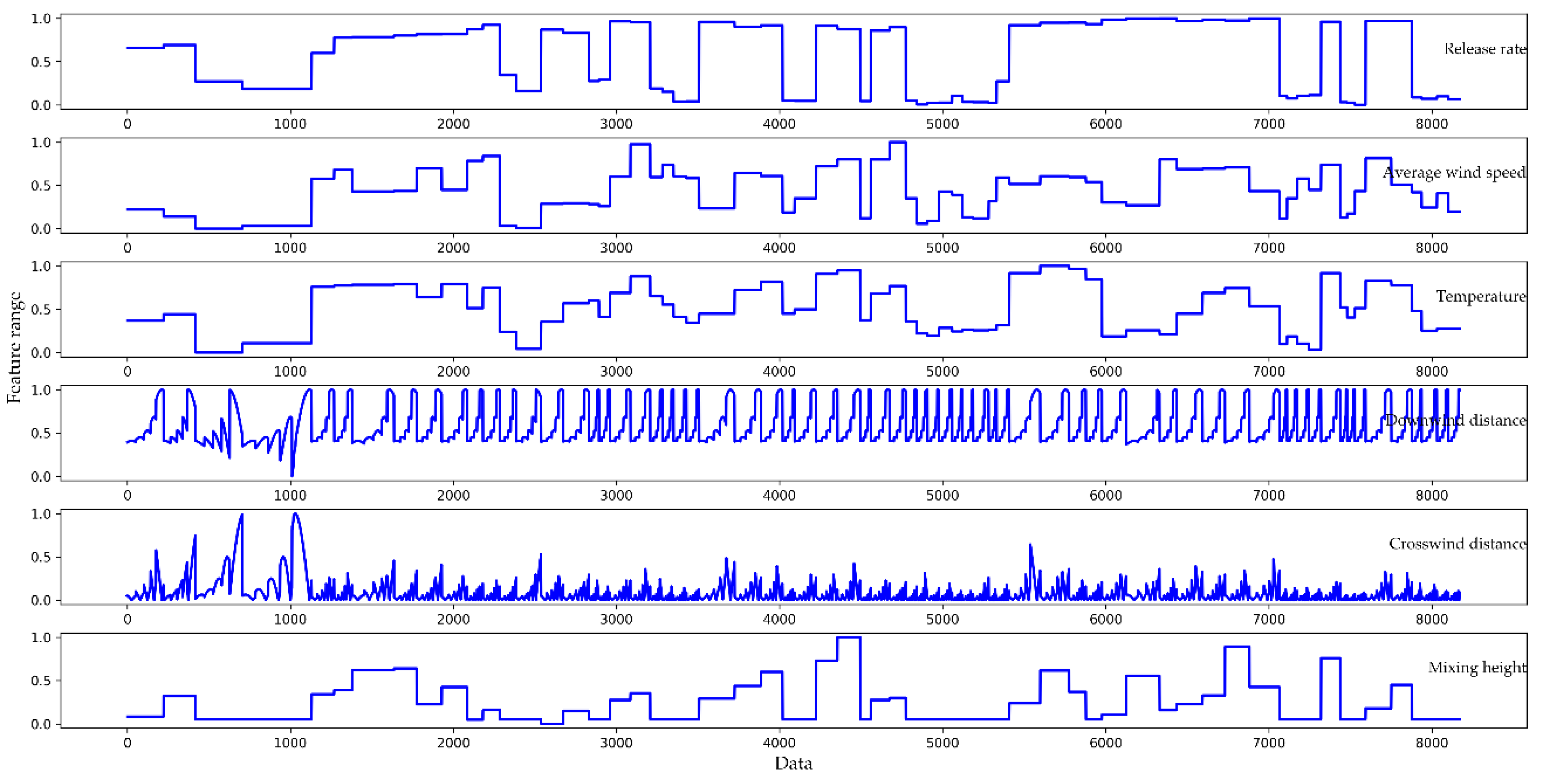
3.1. Data Preprocessing
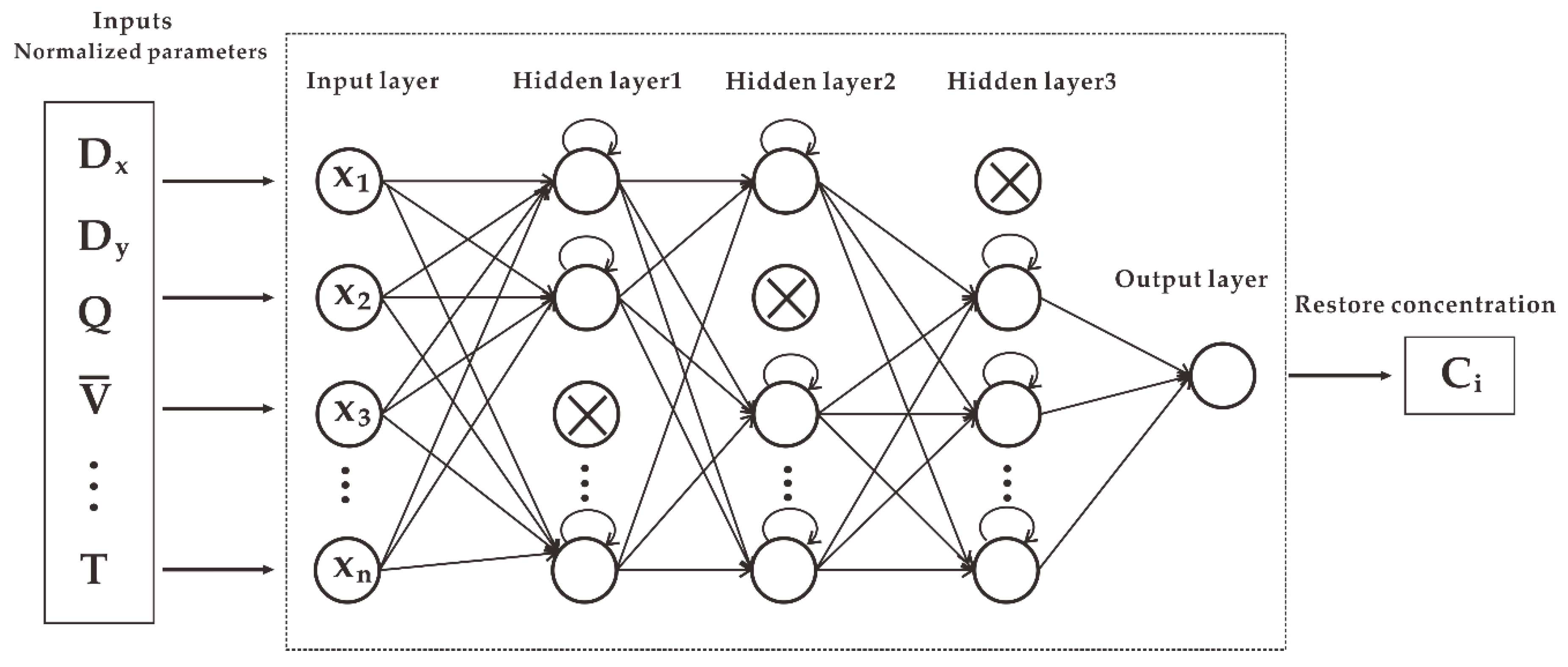
3.2. Model Design
3.3. Performance Criteria
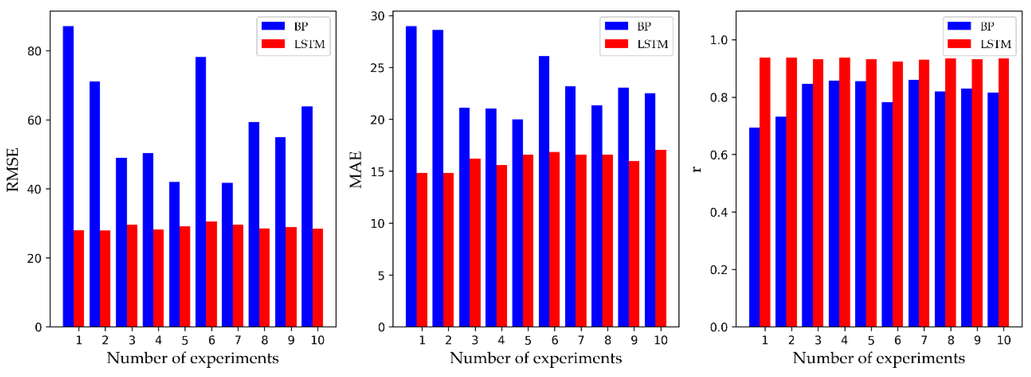
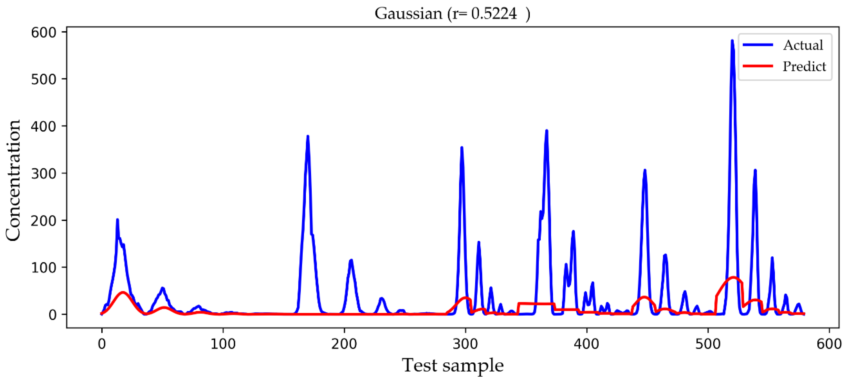
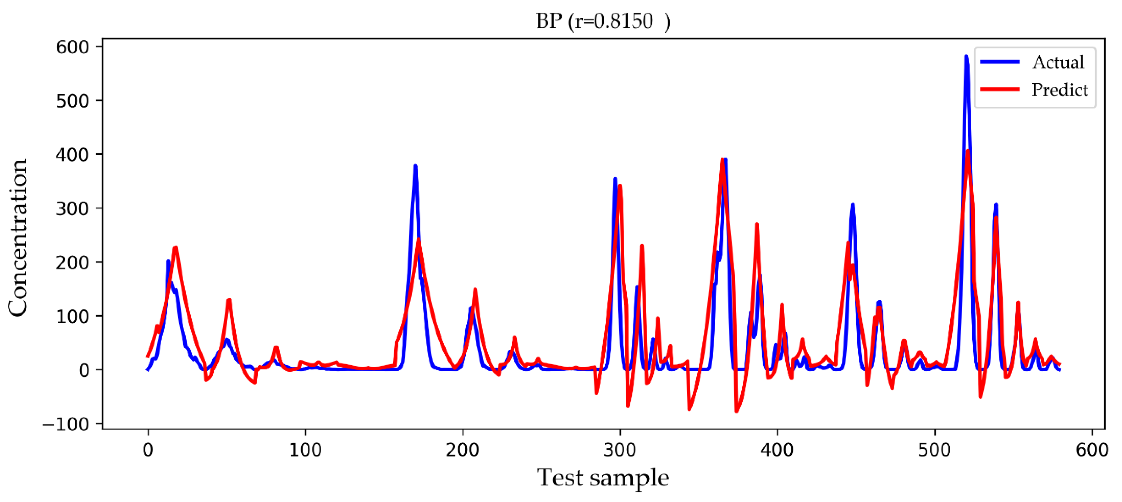
4. Results and Discussion
5. Conclusions
Author Contributions
Funding
Acknowledgments
Conflicts of Interest
References
- Qiu, S.H.; Chen, B.; Wang, R.X.; Zhu, Z.Q.; Wang, Y.; Qiu, X.G. Atmospheric Dispersion Prediction and Source Estimation of Hazardous Gas Using Artificial Neural Network, Particle Swarm Optimization and Expectation Maximization. Atmos. Environ. 2018, 178, 158–163. [Google Scholar] [CrossRef]
- Mazzoldi, A.; Hill, T.; Colls, J.J. Cfd and Gaussian Atmospheric Dispersion Models: A Comparison for Leak from Carbon Dioxide Transportation and Storage Facilities. Atmos. Environ. 2008, 42, 8046–8054. [Google Scholar] [CrossRef]
- Hanna, S.R.; Hansen, O.R.; Ichard, M.; Strimaitis, D. Cfd Model Simulation of Dispersion from Chlorine Railcar Releases in Industrial and Urban Areas. Atmos. Environ. 2009, 43, 262–270. [Google Scholar] [CrossRef]
- Pontiggia, M.; Derudi, M.; Alba, M.; Scaioni, M.; Rota, R. Hazardous Gas Releases in Urban Areas: Assessment of Consequences through Cfd Modelling. J. Hazard. Mater. 2010, 176, 589–596. [Google Scholar] [CrossRef] [PubMed]
- Riddle, A.; Carruthers, D.; Sharpe, A.; McHugh, C.; Stocker, J. Comparisons between Fluent and Adms for Atmospheric Dispersion Modelling. Atmos. Environ. 2004, 38, 1029–1038. [Google Scholar] [CrossRef]
- Wang, B.; Chen, B.Z.; Zhao, J.S. The Real-Time Estimation of Hazardous Gas Dispersion by the Integration of Gas Detectors, Neural Network and Gas Dispersion Models. J. Hazard. Mater. 2015, 300, 433–442. [Google Scholar] [CrossRef]
- Ma, D.L.; Zhang, Z.X. Contaminant Dispersion Prediction and Source Estimation with Integrated Gaussian-Machine Learning Network Model for Point Source Emission in Atmosphere. J. Hazard. Mater. 2016, 311, 237–245. [Google Scholar] [CrossRef] [PubMed]
- Lauret, P.; Heymes, F.; Aprin, L.; Johannet, A. Atmospheric Dispersion Modeling Using Artificial Neural Network Based Cellular Automata. Environ. Model. Softw. 2016, 85, 56–69. [Google Scholar] [CrossRef]
- Na, J.; Jeon, K.; Lee, W.B. Toxic Gas Release Modeling for Real-Time Analysis Using Variational Autoencoder with Convolutional Neural Networks. Chem. Eng. Sci. 2018, 181, 68–78. [Google Scholar] [CrossRef]
- Ni, J.; Yang, H.; Yao, J.; Li, Z.; Qin, P. Toxic Gas Dispersion Prediction for Point Source Emission Using Deep Learning Method. Hum. Ecol. Risk Assess. Int. J. 2019, 1–14. [Google Scholar] [CrossRef]
- Hochreiter, S.; Schmidhuber, J. Long Short-Term Memory. Neural Comput. 1997, 9, 1735–1780. [Google Scholar] [CrossRef] [PubMed]
- Graves, A.; Mohamed, A.R.; Hinton, G. Speech Recognition with Deep Recurrent Neural Networks. In Proceedings of the 2013 IEEE International Conference on Acoustics, Speech and Signal Processing (ICASSP), Vancouver, BC, Canada, 26–31 May 2013; pp. 6645–6649. [Google Scholar]
- Graves, A.; Schmidhuber, J. Framewise Phoneme Classification with Bidirectional Lstm and Other Neural Network Architectures. Neural Netw. 2005, 18, 602–610. [Google Scholar] [CrossRef] [PubMed]
- Sak, H.; Senior, A.; Beaufays, F. Long Short-Term Memory Recurrent Neural Network Architectures for Large Scale Acoustic Modeling. In Proceedings of the 15th Annual Conference of the International Speech Communication Association (INTERSPEECH 2014), Singapore, 14–18 September 2014; pp. 338–342. [Google Scholar]
- Zhao, Z.Y.; Rao, R.N.; Tu, S.X.; Shi, J. Time-Weighted Lstm Model with Redefined Labeling for Stock Trend Prediction. In Proceedings of the 2017 IEEE 29th International Conference on Tools with Artificial Intelligence (Ictai 2017), Boston, MA, USA, 6–8 November 2017; pp. 1210–1217. [Google Scholar]
- Liu, H.; Mi, X.W.; Li, Y.F. Smart Multi-Step Deep Learning Model for Wind Speed Forecasting Based on Variational Mode Decomposition, Singular Spectrum Analysis, Lstm Network and Elm. Energy Convers. Manag. 2018, 159, 54–64. [Google Scholar] [CrossRef]
- Qing, X.Y.; Niu, Y.G. Hourly Day-Ahead Solar Irradiance Prediction Using Weather Forecasts by Lstm. Energy 2018, 148, 461–468. [Google Scholar] [CrossRef]
- Besnard, S.; Carvalhais, N.; Arain, M.A.; Black, A.; Brede, B.; Buchmann, N.; Chen, J.Q.; Clevers, J.G.P.W.; Dutrieux, L.P.; Gans, F.; et al. Memory Effects of Climate and Vegetation Affecting Net Ecosystem CO2 Fluxes in Global Forests. PLoS ONE 2019, 14, e0213467. [Google Scholar] [CrossRef] [PubMed]
- Zhang, T.J.; Song, S.; Li, S.G.; Ma, L.; Pan, S.B.; Han, L.Y. Research on Gas Concentration Prediction Models Based on Lstm Multidimensional Time Series. Energies 2019, 12, 161. [Google Scholar] [CrossRef]
- Huang, C.J.; Kuo, P.H. A Deep Cnn-Lstm Model for Particulate Matter (PM2.5) Forecasting in Smart Cities. Sensors 2018, 18, 2220. [Google Scholar] [CrossRef]
- Zhao, J.C.; Deng, F.; Cai, Y.Y.; Chen, J. Long Short-Term Memory–Fully Connected (Lstm-Fc) Neural Network for PM2.5 Concentration Prediction. Chemosphere 2019, 220, 486–492. [Google Scholar] [CrossRef]
- Hyunseung, K.; Park, M.; Kim, C.W.; Shin, D. Source Localization for Hazardous Material Release in an Outdoor Chemical Plant Via a Combination of Lstm-Rnn and Cfd Simulation. Comput. Chem. Eng. 2019, 125, 476–489. [Google Scholar]
- Barad, M.L. Project Prairie Grass, a Field Program in Diffusion I; Air Force Cambridge Research Center: Cambridge, MA, USA, 1958. [Google Scholar]
- Barad, M.L. Project Prairie Grass, a Field Program in Diffusion II; Air Force Cambridge Research Center: Cambridge, MA, USA, 1958. [Google Scholar]
- Sawford, B.L. Project Prairie Grass—A Classic Atmospheric Dispersion Experiment Revisited. In Proceedings of the 14th Australasian Fluid Mechanics Conference, Adelaide, Australia, 10–14 December 2001; pp. 175–178. [Google Scholar]
- Razvan, P.; Mikolov, T.; Bengio, Y. On the Difficulty of Training Recurrent Neural Networks. In Proceedings of the 30th International Conference on Machine Learning, Atlanta, GA, USA, 16–21 June 2013; Volume 28, pp. 1310–1318. [Google Scholar]
- Bengio, Y.; Simard, P.; Frasconi, P. Learning Long-Term Dependencies with Gradient Descent Is Difficult. IEEE Trans. Neural Netw. 1994, 5, 157–166. [Google Scholar] [CrossRef]
- Hawkins, D.M. The Problem of Overfitting. J. Chem. Inf. Comput. Sci. 2004, 44, 1–12. [Google Scholar] [CrossRef] [PubMed]
- Srivastava, N.; Hinton, G.; Krizhevsky, A.; Sutskever, I.; Salakhutdinov, R. Dropout: A Simple Way to Prevent Neural Networks from Overfitting. J. Mach. Learn. Res. 2014, 15, 1929–1958. [Google Scholar]
- Tangadpalliwar, S.R.; Vishwakarma, S.; Nimbalkar, R.; Garg, P. Chemsuite: A Package for Chemoinformatics Calculations and Machine Learning. Chem. Biol. Drug Des. 2019, 93, 960–964. [Google Scholar] [CrossRef] [PubMed]
- Cao, X.H.; Stojkovic, I.; Obradovic, Z. A Robust Data Scaling Algorithm to Improve Classification Accuracies in Biomedical Data. BMC Bioinf. 2016, 17, 359. [Google Scholar] [CrossRef] [PubMed]
- Xu, L.; Choy, C.S.; Li, Y.W. Deep Sparse Rectifier Neural Networks for Speech Denoising. In Proceedings of the 2016 IEEE International Workshop on Acoustic Signal Enhancement (Iwaenc), Xi’an, China, 13–16 September 2016. [Google Scholar]
- Chai, T.; Draxler, R.R. Root Mean Square Error (Rmse) or Mean Absolute Error (Mae)?—Arguments against Avoiding Rmse in the Literature. Geosci. Model Dev. 2014, 7, 1247–1250. [Google Scholar] [CrossRef]
- Willmott, C.J.; Matsuura, K. Advantages of the Mean Absolute Error (Mae) over the Root Mean Square Error (Rmse) in Assessing Average Model Performance. Clim. Res. 2005, 30, 79–82. [Google Scholar] [CrossRef]
- Xin, G.; Li, X.; Zhao, B.; Ji, W.; Jing, X.; He, Y. Short-Term Electricity Load Forecasting Model Based on Emd-Gru with Feature Selection. Energies 2019, 12, 1140. [Google Scholar]
- Joseph, L.R.; Nicewander, W.A. Thirteen Ways to Look at the Correlation Coefficient. Am. Stat. 1988, 42, 59–66. [Google Scholar]
- Wang, R.X.; Chen, B.; Qiu, S.H.; Zhu, Z.Q.; Wang, Y.D.; Wang, Y.P.; Qiu, X.G. Comparison of Machine Learning Models for Hazardous Gas Dispersion Prediction in Field Cases. Int. J. Environ. Res. Public Health 2018, 15, 1450. [Google Scholar] [CrossRef]


| Parameters | Symbol | Unit |
|---|---|---|
| Downwind distance | Dx | m |
| Crosswind distance | Dy | m |
| Wind direction | θ | ° |
| Average wind speed | m/s | |
| Version number | No | / |
| Release rate | Q | g/s |
| Height of source | H | m |
| Temperature | T | °C |
| Height of interest point | Zo | m |
| Mixing height | Zm | m |
| Heat flux | Hf | W/m2 |
| Atmosphere stability length | L | m |
| Models | RMSE | MAE | r |
|---|---|---|---|
| Gaussian | 78.6877 | 34.5548 | 0.5224 |
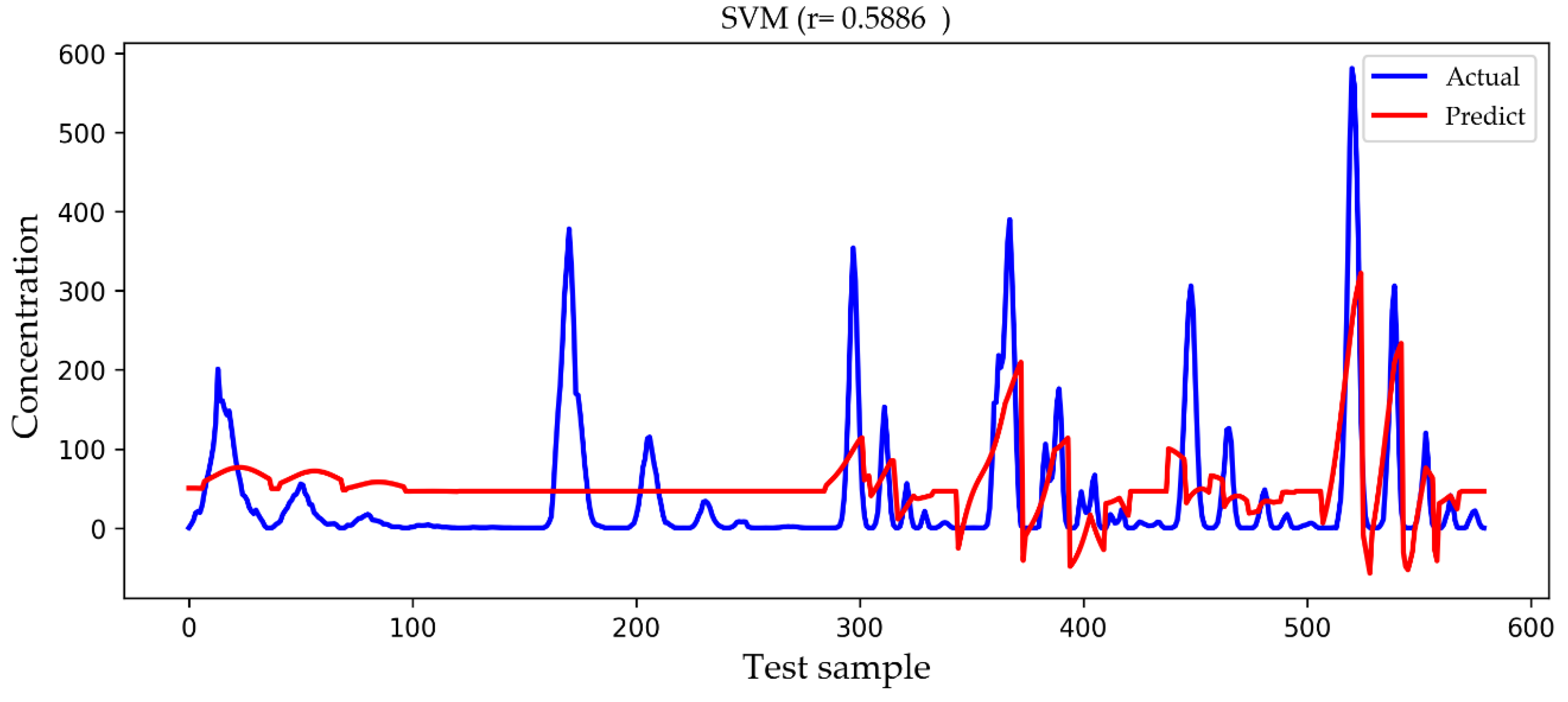
| SVM | 50.9144 | 67.0491 | 0.5886 |
| BP | 59.7562 | 23.5882 | 0.8093 |
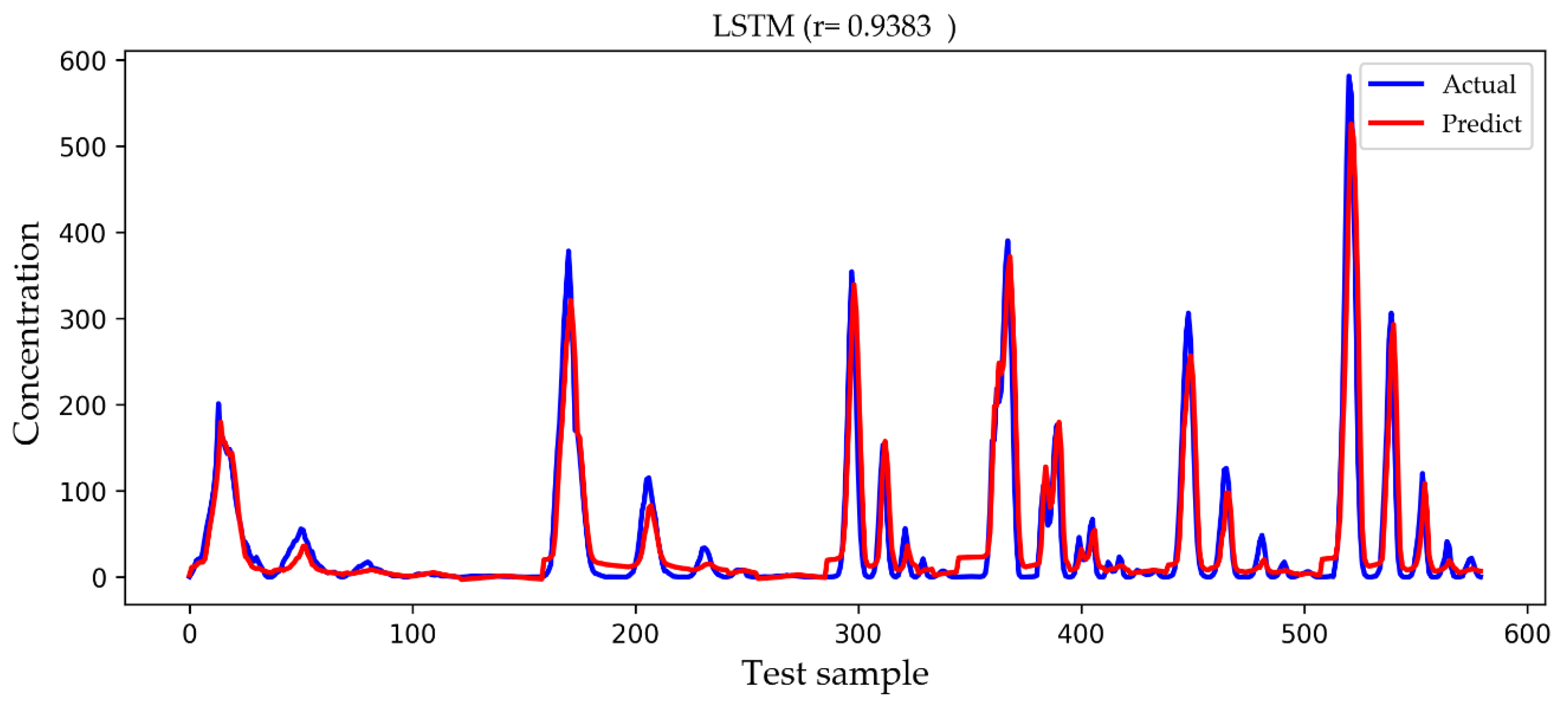
| LSTM | 28.9063 | 16.1069 | 0.9338 |
© 2019 by the authors. Licensee MDPI, Basel, Switzerland. This article is an open access article distributed under the terms and conditions of the Creative Commons Attribution (CC BY) license (http://creativecommons.org/licenses/by/4.0/).
Share and Cite
Qian, F.; Chen, L.; Li, J.; Ding, C.; Chen, X.; Wang, J. Direct Prediction of the Toxic Gas Diffusion Rule in a Real Environment Based on LSTM. Int. J. Environ. Res. Public Health 2019, 16, 2133. https://doi.org/10.3390/ijerph16122133
Qian F, Chen L, Li J, Ding C, Chen X, Wang J. Direct Prediction of the Toxic Gas Diffusion Rule in a Real Environment Based on LSTM. International Journal of Environmental Research and Public Health. 2019; 16(12):2133. https://doi.org/10.3390/ijerph16122133
Chicago/Turabian StyleQian, Fei, Li Chen, Jun Li, Chao Ding, Xianfu Chen, and Jian Wang. 2019. "Direct Prediction of the Toxic Gas Diffusion Rule in a Real Environment Based on LSTM" International Journal of Environmental Research and Public Health 16, no. 12: 2133. https://doi.org/10.3390/ijerph16122133
APA StyleQian, F., Chen, L., Li, J., Ding, C., Chen, X., & Wang, J. (2019). Direct Prediction of the Toxic Gas Diffusion Rule in a Real Environment Based on LSTM. International Journal of Environmental Research and Public Health, 16(12), 2133. https://doi.org/10.3390/ijerph16122133