Machine Learning-Based Integration of High-Resolution Wildfire Smoke Simulations and Observations for Regional Health Impact Assessment

 , ,
, ,  , and
, and
Abstract
1. Introduction
2. Data Materials and Modeling Methods
- (1)
- Step 1: Gap filling for spatiotemporal missing values in the Multi-Angle Implementation of Atmospheric Correction (MAIAC) satellite AOD retrievals [34]. This was based on (1) three hourly meteorological variables including total cloud fraction, cloud liquid water content, and surface water vapor mixing ratio from the WRF outputs, (2) two geographical variables including terrain elevation and vegetation coverage, and (3) the simulated hourly AOD from the WRF-CMAQ SENS experiment;
- (2)
- Step 2: Data fusion for optimizing daily surface PM2.5 concentrations from the WRF-CMAQ SENS experiment, based on (1) daily averages of observational AirNow surface PM2.5 measurements, (2) gap-filled AOD from Step 1, and (3) six meteorological variables, including surface wind speed and directions at 10 m, surface air temperature at 2 m, relative humidity at 2 m, precipitation rates at surface on a log scale, and planetary boundary layer heights from the North American Regional Reanalysis (NARR) data [35] produced by the National Centers for Environmental Prediction.
3. Observational and Modeling Results
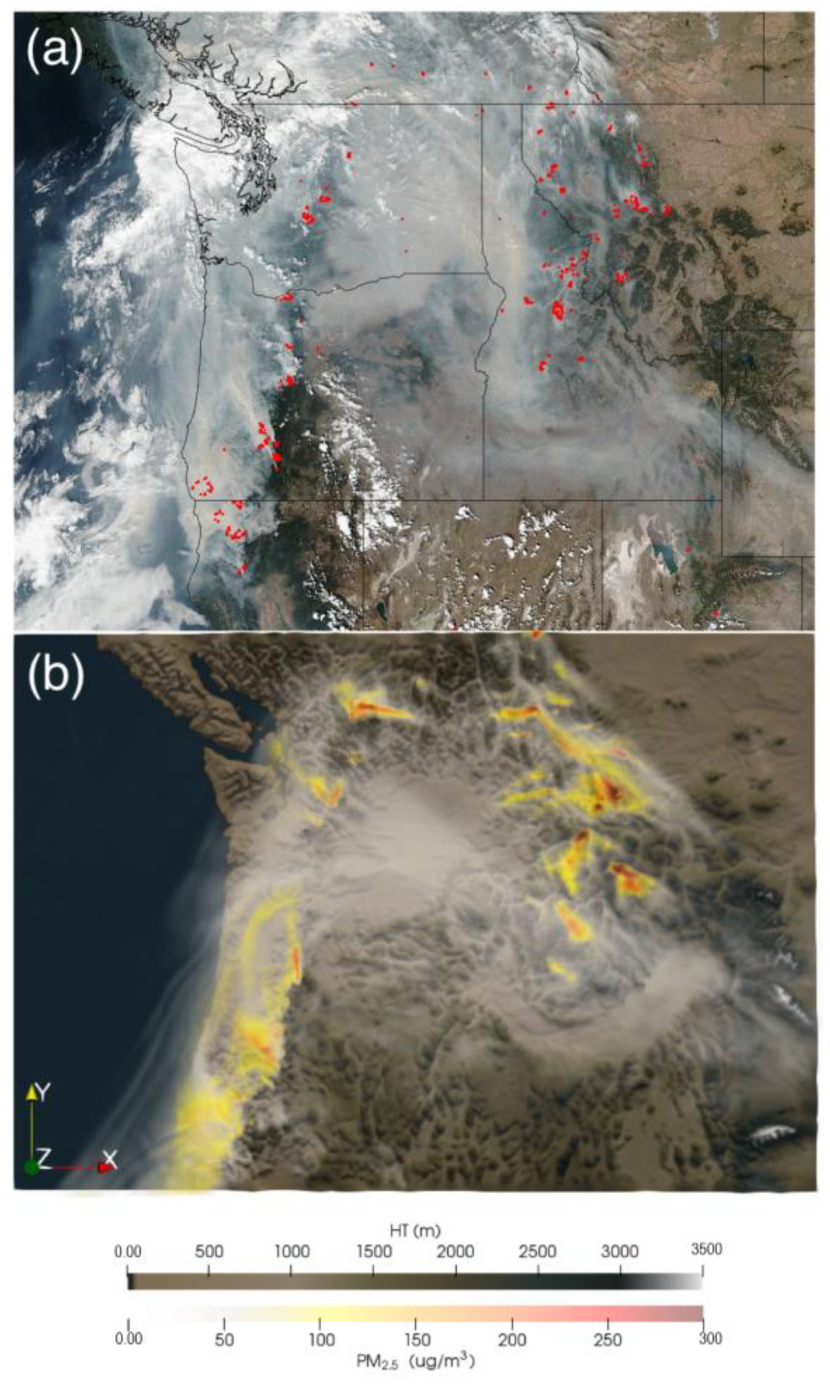
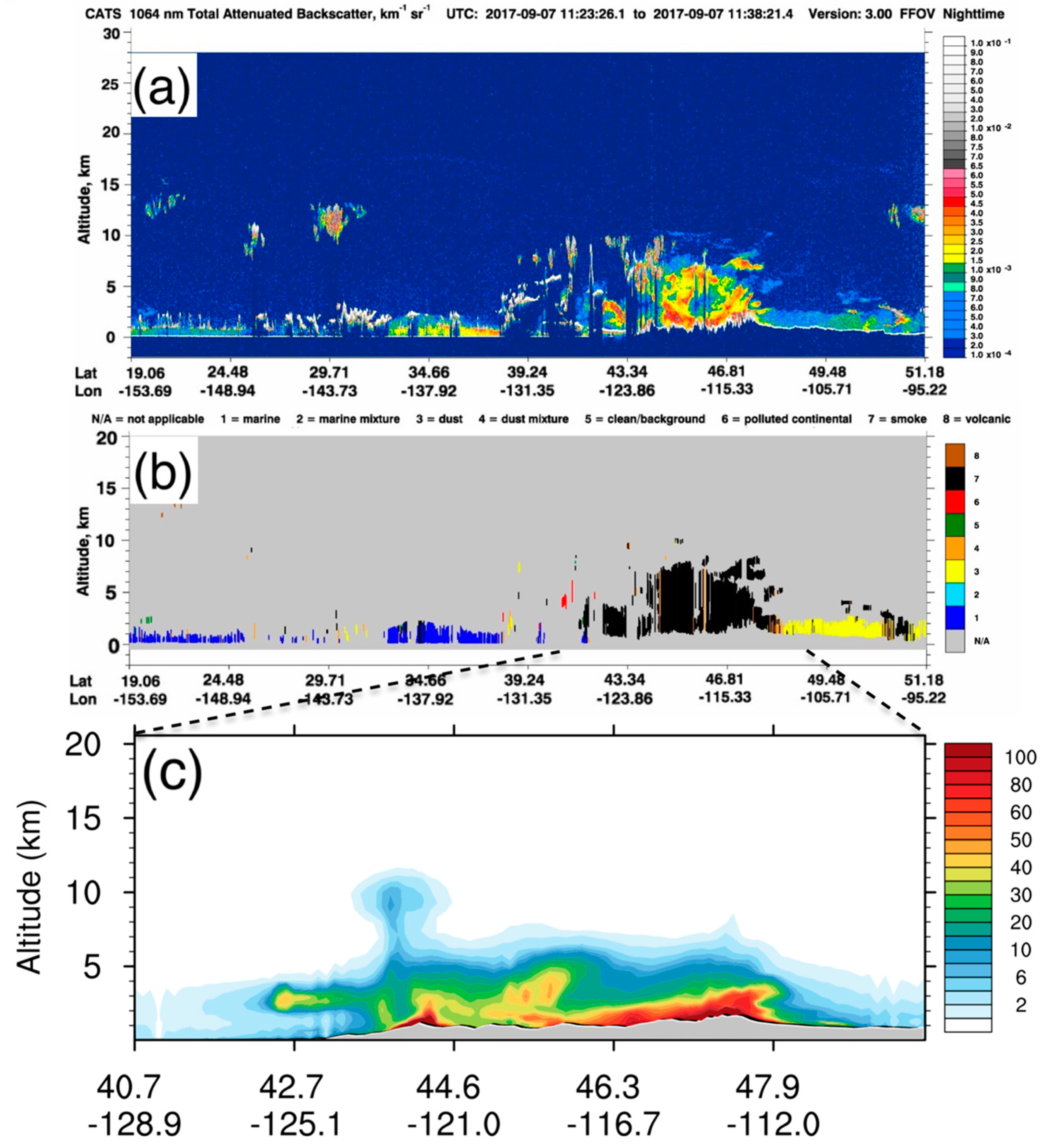
3.1. The 2017 PNW Fire Smoke Pollution Episode
3.2. Model Simulation and Evalution Results
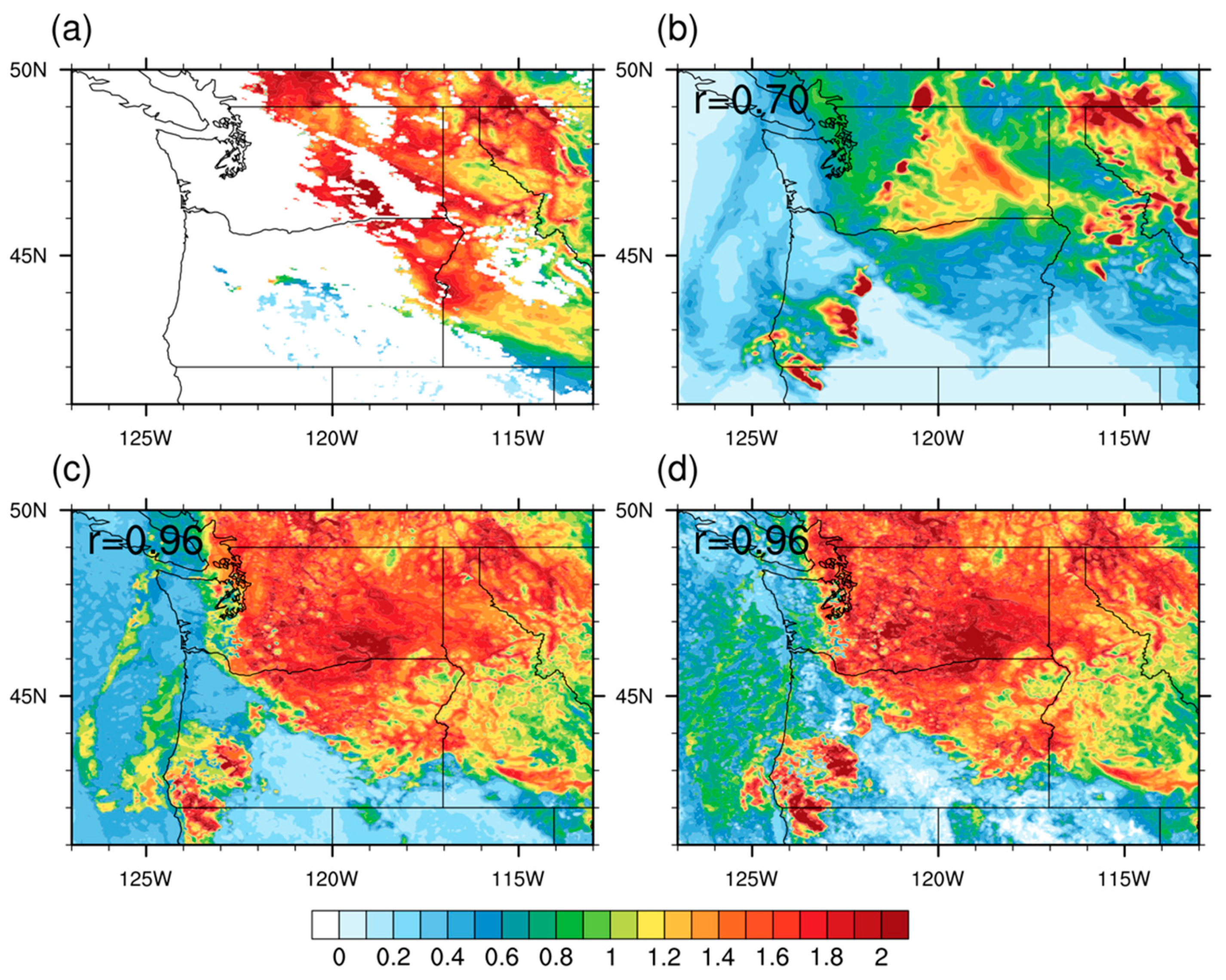
3.2.1. Gap-Filling for MAIAC AOD
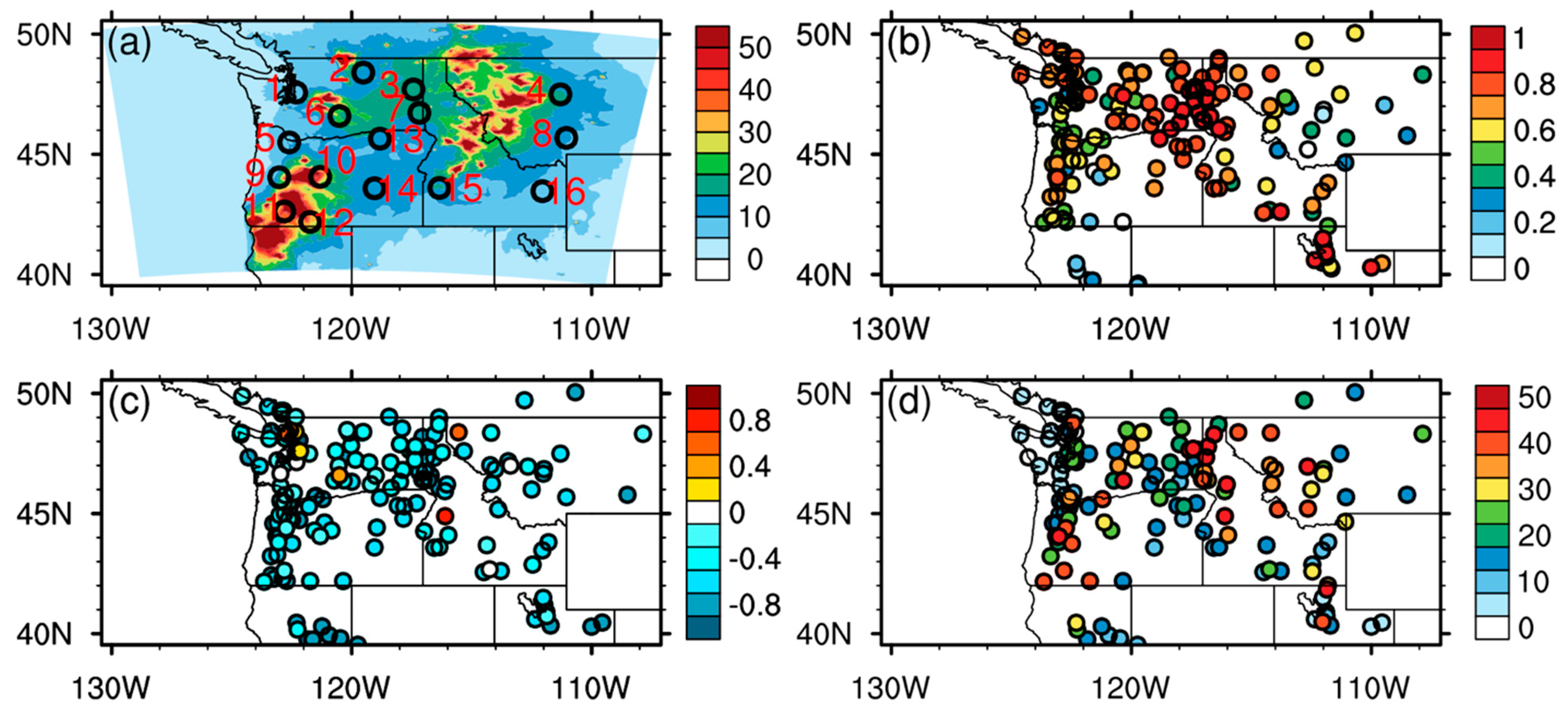
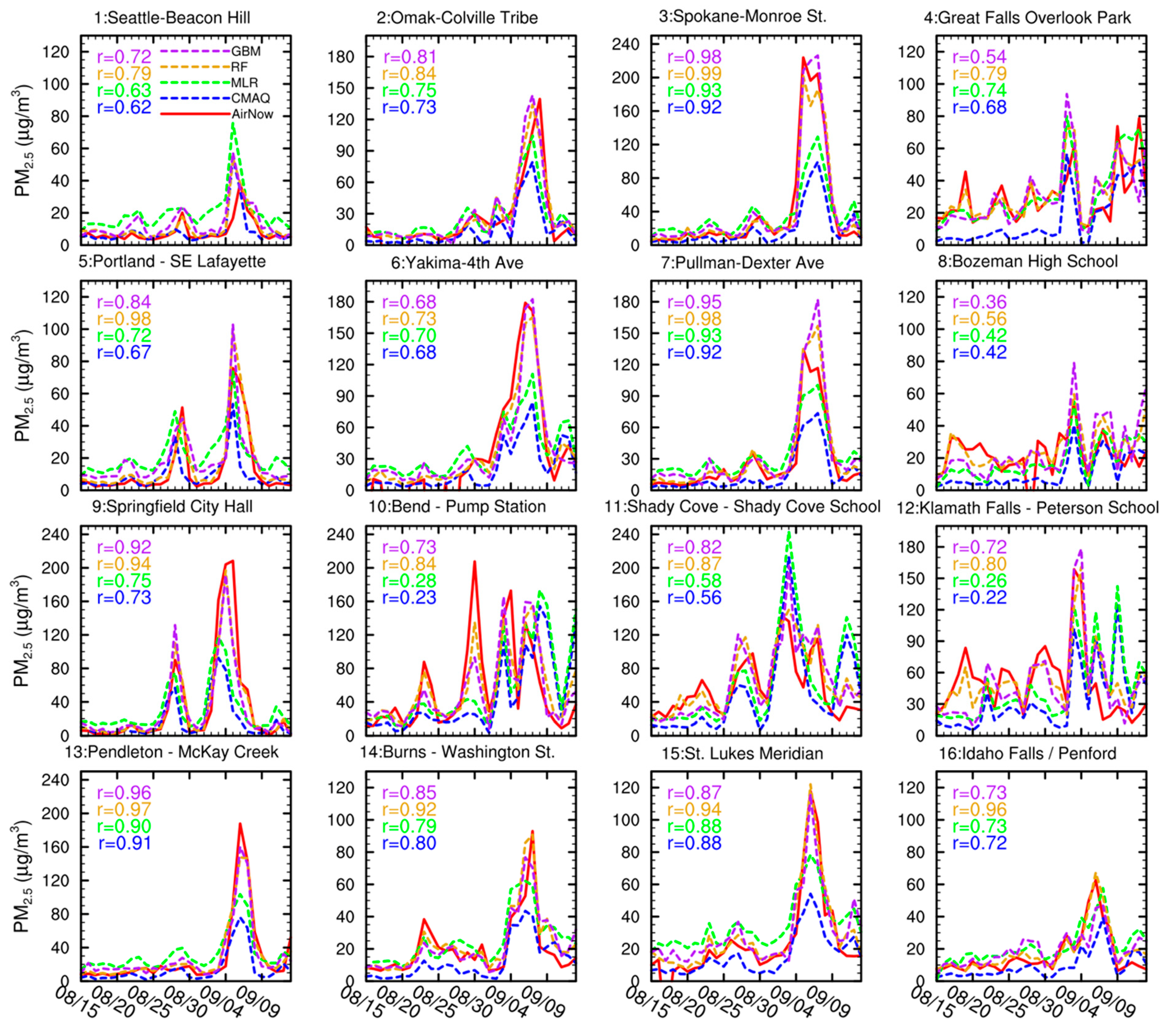
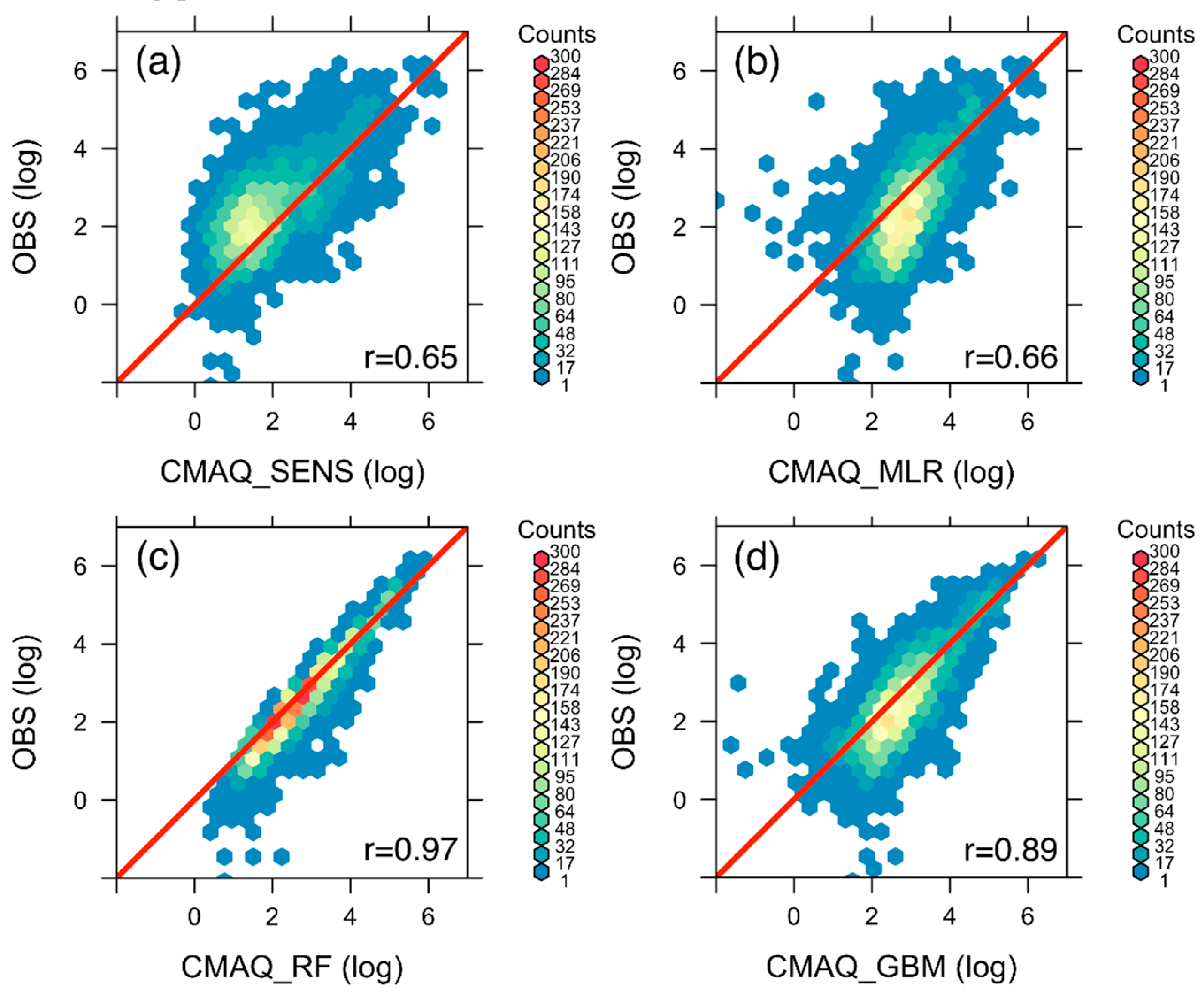
3.2.2. Data Fusion for Surface PM2.5 Concentrations
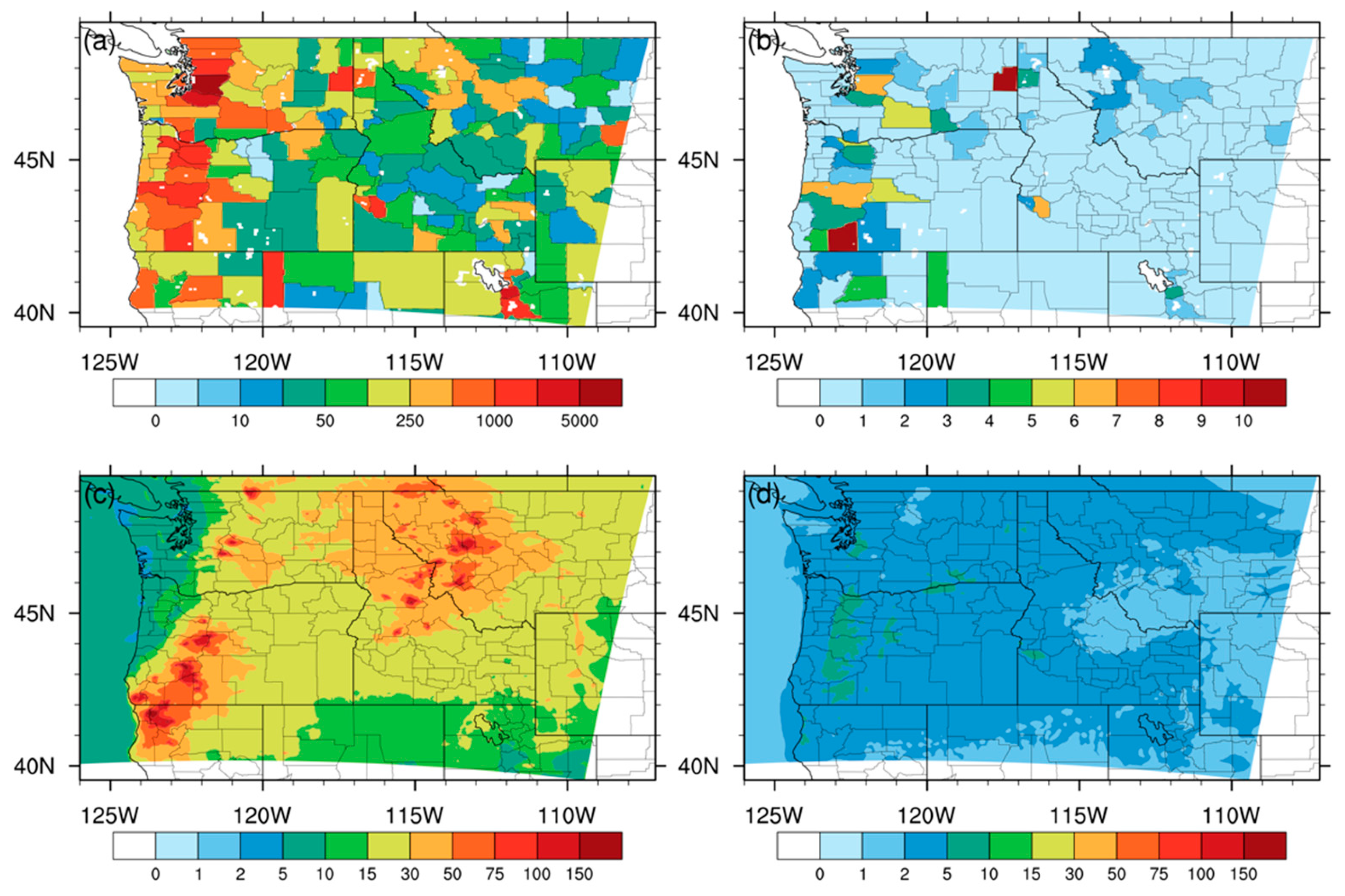
3.3. Regional Health Impact Assessment
4. Discussion
5. Conclusions
Supplementary Materials
Author Contributions
Funding
Acknowledgments
Conflicts of Interest
References
- Johnston, F.H.; Henderson, S.B.; Chen, Y.; Randerson, J.T.; Marlier, M.; DeFries, R.S.; Kinney, P.; Bowman, D.M.J.S.; Brauer, M. Estimated global mortality attributable to smoke from landscape fires. Environ. Health Persp. 2012, 120, 695–701. [Google Scholar] [CrossRef] [PubMed]
- Fann, N.; Alman, B.; Broome, R.A.; Morgan, G.G.; Johnston, F.H.; Pouliot, G.; Rappold, A.G. The health impacts and economic value of wildland fire episodes in the U.S.: 2008–2012. Sci. Total Environ. 2018, 610–611, 802–809. [Google Scholar] [CrossRef] [PubMed]
- Liu, Y.Q. Variability of wildland fire emissions across the contiguous United States. Atmos. Environ. 2004, 38, 3489–3499. [Google Scholar] [CrossRef]
- Reid, C.E.; Brauer, M.; Johnston, F.H.; Jerrett, M.; Balmes, J.R.; Elliott, C.T. Critical review of health impacts of wildfire smoke exposure. Environ. Health Persp. 2016, 124, 1334–1343. [Google Scholar] [CrossRef] [PubMed]
- Kondo, M.C.; De Roos, A.J.; White, L.S.; Heilman, W.E.; Mockrin, M.H.; Gross-Davis, C.A.; Burstyn, I. Meta-analysis of heterogeneity in the effects of wildfire smoke exposure on respiratory health in North America. Int. J. Environ. Res. Public Health 2019, 16, 960. [Google Scholar] [CrossRef] [PubMed]
- Navarro, K.M.; Schweizer, D.; Balmes, J.R.; Cisneros, R. A review of community smoke exposure from wildfire compared to prescribed fire in the United States. Atmosphere 2018, 9, 185. [Google Scholar] [CrossRef]
- Cascio, W.E. Wildland fire smoke and human health. Sci. Total Environ. 2018, 624, 586–595. [Google Scholar] [CrossRef] [PubMed]
- Rappold, A.G.; Reyes, J.; Pouliot, G.; Cascio, W.E.; Diaz-Sanchez, D. Community vulnerability to health impacts of wildland fire smoke exposure. Environ. Sci. Technol. 2017, 51, 6674–6682. [Google Scholar] [CrossRef]
- 2017 Pacific Northwest Fire Narrative. 2018; p. 128. Available online: https://www.fs.usda.gov/Internet/FSE_DOCUMENTS/fseprd572804.pdf (accessed on 26 March 2019).
- McClure, C.D.; Jaffe, D.A. US particulate matter air quality improves except in wildfire-prone areas. Proc. Natl. Acad. Sci. USA 2018, 115, 7901–7906. [Google Scholar] [CrossRef]
- Strand, T.; Larkin, N.; Rorig, M.; Krull, C.; Moore, M. PM2.5 measurements in wildfire smoke plumes from fire seasons 2005–2008 in the Northwestern United States. J. Aerosol Sci. 2011, 42, 143–155. [Google Scholar] [CrossRef]
- Larkin, N.K.; O’Neill, S.M.; Solomon, R.; Raffuse, S.; Strand, T.; Sullivan, D.C.; Krull, C.; Rorig, M.; Peterson, J.L.; Ferguson, S.A. The BlueSky smoke modeling framework. Int. J. Wildland Fire 2009, 18, 906–920. [Google Scholar] [CrossRef]
- Herron-Thorpe, F.L.; Lamb, B.K.; Mount, G.H.; Vaughan, J.K. Evaluation of a regional air quality forecast model for tropospheric NO2 columns using the OMI/Aura satellite tropospheric NO2 product. Atmos. Chem. Phys. 2010, 10, 8839–8854. [Google Scholar] [CrossRef]
- Chen, J.; Vaughan, J.; Avise, J.; O’Neill, S.; Lamb, B. Enhancement and evaluation of the AIRPACT ozone and PM2.5 forecast system for the Pacific Northwest. J. Geophys. Res.-Atmos. 2008, 113. [Google Scholar] [CrossRef]
- Pillar, E.A.; Camm, R.C.; Guzman, M.I. Catechol oxidation by ozone and hydroxyl radicals at the air-water interface. Environ. Sci. Technol. 2014, 48, 14352–14360. [Google Scholar] [CrossRef] [PubMed]
- Pillar, E.A.; Guzman, M.I. Oxidation of substituted catechols at the air-water interface: Production of carboxylic acids, quinones, and polyphenols. Environ. Sci. Technol. 2017, 51, 4951–4959. [Google Scholar] [CrossRef] [PubMed]
- Magalhaes, A.C.O.; da Silva, J.C.G.E.; da Silva, L.P. Density functional theory calculation of the absorption properties of brown carbon chromophores generated by catechol heterogeneous ozonolysis. Acs. Earth Space Chem. 2017, 1, 353–360. [Google Scholar] [CrossRef]
- Yu, L.; Smith, J.; Laskin, A.; George, K.M.; Anastasio, C.; Laskin, J.; Dillner, A.M.; Zhang, Q. Molecular transformations of phenolic SOA during photochemical aging in the aqueous phase: competition among oligomerization, functionalization, and fragmentation. Atmos. Chem. Phys. 2016, 16, 4511–4527. [Google Scholar] [CrossRef]
- Lavi, A.; Lin, P.; Bhaduri, B.; Carmieli, R.; Laskin, A.; Rudich, Y. Characterization of light-absorbing oligomers from phenolic compounds and Fe(III). Acs. Earth Space Chem. 2017, 1, 637–646. [Google Scholar] [CrossRef]
- Smith, J.D.; Kinney, H.; Anastasio, C. Phenolic carbonyls undergo rapid aqueous photodegradation to form low-volatility, light-absorbing products. Atmos. Environ. 2016, 126, 36–44. [Google Scholar] [CrossRef]
- Sun, J.; Mei, Q.; Wei, B.; Huan, L.; Xie, J.; He, M. Mechanisms for ozone-initiated removal of biomass burning products from the atmosphere. Environ. Chem. 2018, 15, 83–91. [Google Scholar] [CrossRef]
- Koo, B.; Knipping, E.; Yarwood, G. 1.5-Dimensional volatility basis set approach for modeling organic aerosol in CAMx and CMAQ. Atmos. Environ. 2014, 95, 158–164. [Google Scholar] [CrossRef]
- Woody, M.C.; Baker, K.R.; Hayes, P.L.; Jimenez, J.L.; Koo, B.; Pye, H.O.T. Understanding sources of organic aerosol during CalNex-2010 using the CMAQ-VBS. Atmos. Chem. Phys. 2016, 16, 4081–4100. [Google Scholar] [CrossRef]
- Black, C.; Tesfaigzi, Y.; Bassein, J.A.; Miller, L.A. Wildfire smoke exposure and human health: Significant gaps in research for a growing public health issue. Environ. Toxicol. Phar. 2017, 55, 186–195. [Google Scholar] [CrossRef] [PubMed]
- Liu, J.C.; Pereira, G.; Uhl, S.A.; Bravo, M.A.; Bell, M.L. A systematic review of the physical health impacts from non-occupational exposure to wildfire smoke. Environ. Res. 2015, 136, 120–132. [Google Scholar] [CrossRef] [PubMed]
- Youssouf, H.; Liousse, C.; Roblou, L.; Assamoi, E.M.; Salonen, R.O.; Maesano, C.; Banerjee, S.; Annesi-Maesano, I.; Study, P. Quantifying wildfires exposure for investigating health-related effects. Atmos. Environ. 2014, 97, 239–251. [Google Scholar] [CrossRef]
- Skamarock, W.C.; Klemp, J.B.; Dudhia, J.; Gill, D.O.; Barker, D.M.; Duda, M.G.; Huang, X.-Y.; Wang, W.; Powers, J.G. A Description of the Advanced Research WRF Version 3; NCAR: Boulder, CO, USA, 2008; p. 113. [Google Scholar]
- CMASwiki Contributors, CMAQ Version 5.2 (June 2017 Release) Technical Documentation. Available online: https://www.airqualitymodeling.org/index.php/CMAQ_version_5.2_(June_2017_release)_Technical_Documentation (accessed on 26 March 2019).
- Wong, D.C.; Pleim, J.; Mathur, R.; Binkowski, F.; Otte, T.; Gilliam, R.; Pouliot, G.; Xiu, A.; Young, J.O.; Kang, D. WRF-CMAQ two-way coupled system with aerosol feedback: Software development and preliminary results. Geosci. Model. Dev. 2012, 5, 299–312. [Google Scholar] [CrossRef]
- Goodrick, S.L.; Achtemeier, G.L.; Larkin, N.K.; Liu, Y.Q.; Strand, T.M. Modelling smoke transport from wildland fires: A review. Int. J. Wildland Fire 2013, 22, 83–94. [Google Scholar] [CrossRef]
- Baek, B.H. Sparse Matrix Operator Kerner Emissions (SMOKE) Modeling System, the Community Modeling and Analysis System Center: The Center for Environmental Modeling for Policy Development (CEMPD) at the University of North Carolina at Chapel Hill. 2018. Available online: https://www.cmascenter.org/smoke/ (accessed on 26 March 2019). [CrossRef]
- The U.S. Environmental Protection Agency. 2014 National Emissions Inventory (NEI) Data; The U.S. EPA, Ed.; The U.S. Environmental Protection Agency: Washington, WA, USA, 2015.
- Reid, C.E.; Jerrett, M.; Petersen, M.L.; Pfister, G.G.; Morefield, P.E.; Tager, I.B.; Raffuse, S.M.; Balmes, J.R. Spatiotemporal prediction of fine particulate matter during the 2008 Northern California wildfires using machine learning. Environ. Sci. Technol. 2015, 49, 3887–3896. [Google Scholar] [CrossRef]
- Lyapustin, A.; Wang, Y. MCD19A2 MODIS/Terra+Aqua Land Aerosol Optical Depth Daily L2G Global 1km SIN Grid V006 DAAC. NASA EOSDIS Land Processes DAAC. Available online: https://lpdaac.usgs.gov/products/mcd19a2v006/ (accessed on 26 March 2019). [CrossRef]
- NCEP North American Regional Reanalysis (NARR). Research Data Archive at the National Center for Atmospheric Research; Computational and Information Systems Laboratory: Boulder, CO, USA, 2005. [Google Scholar]
- Everitt, B.S.; Hothorn, T. Multiple linear regression: Cloud seeding, A Handbook of Statistical Analyses Using R. Available online: http://www.ecostat.unical.it/tarsitano/Didattica/LabStat2/Everitt.pdf, 2006 (accessed on 26 March 2019).
- Greenwell, B.; Boehmke, B.; Cunningham, J.; Developers, G. Generalized Boosted Regression Models. Available online: https://cran.r-project.org/web/packages/gbm/index.html (accessed on 26 March 2019).
- Liaw, A.; Wiener, M. Classification and regression by randomForest. R. News 2002, 2, 18–22. [Google Scholar]
- Hanson, H.; McGill, M.; Yorks, J. CATS: Measuring Clouds and Aerosols from the International Space Station; National Aeronautics and Space Administration: Washington, WA, USA, 2014; p. 16.
- Xiao, Q.; Wang, Y.; Chang, H.H.; Meng, X.; Geng, G.; Lyapustin, A.; Liu, Y. Full-coverage high-resolution daily PM2.5 estimation using MAIAC AOD in the Yangtze River Delta of China. Remote Sens. Environ. 2017, 199, 437–446. [Google Scholar] [CrossRef]
- Fann, N.; Lamson, A.D.; Anenberg, S.C.; Wesson, K.; Risley, D.; Hubbell, B.J. Estimating the national public health burden associated with exposure to ambient PM2.5 and ozone. Risk Anal. 2012, 32, 81–95. [Google Scholar] [CrossRef] [PubMed]
- Pope III, C.A.; Burnett, R.T.; Turner, M.C.; Cohen, A.; Krewski, D.; Jerrett, M.; Gapstur, S.M.; Thun, M.J. Lung Cancer and Cardiovascular Disease mortality associated with ambient air pollution and cigarette smoke: Shape of the exposure—Response relationships. Environ. Health Persp. 2011, 119, 1616–1621. [Google Scholar] [CrossRef] [PubMed]
- Center for International Earth Science Information Network—CIESIN—Columbia University. U.S. Census Grids (Summary File 1), 2010; NASA Socioeconomic Data and Applications Center (SEDAC): Palisades, NY, USA, 2017.
- Selimovic, V.; Yokelson, R.J.; McMeeking, G.R.; Coefield, S. In situ measurements of trace gases, PM, and aerosol optical properties during the 2017 NW US wildfire smoke event. Atmos. Chem. Phys. 2019, 19, 3905–3926. [Google Scholar] [CrossRef]
- Bi, J.; Belle, J.H.; Wang, Y.; Lyapustin, A.I.; Wildani, A.; Liu, Y. Impacts of snow and cloud covers on satellite-derived PM2.5 levels. Remote Sens. Environ. 2019, 221, 665–674. [Google Scholar] [CrossRef]
- Briggs, G.A. A plume rise model compared with observations. J. Air Pollut. Cont. Assoc. 1965, 15, 433–438. [Google Scholar] [CrossRef]
- Paugam, R.; Wooster, M.; Freitas, S.; Martin, M.V. A review of approaches to estimate wildfire plume injection height within large-scale atmospheric chemical transport models. Atmos. Chem. Phys. 2016, 16, 907–925. [Google Scholar] [CrossRef]
- Timonen, H.; Wigder, N.; Jaffe, D. Influence of background particulate matter (PM) on urban air quality in the Pacific Northwest. J. Environ. Manage. 2013, 129, 333–340. [Google Scholar] [CrossRef]
- Henderson, S.B.; Brauer, M.; MacNab, Y.C.; Kennedy, S.M. Three measures of forest fire smoke exposure and their associations with respiratory and cardiovascular health outcomes in a population-based cohort. Environ. Health Persp. 2011, 119, 1266–1271. [Google Scholar] [CrossRef]
- Haikerwal, A.; Akram, M.; Del Monaco, A.; Smith, K.; Sim, M.R.; Meyer, M.; Tonkin, A.M.; Abramson, M.J.; Dennekamp, M. Impact of fine particulate matter (PM2.5) exposure during wildfires on cardiovascular health outcomes. J. Am. Heart Assoc. 2015, 4. [Google Scholar] [CrossRef]
- Jaffe, D.A.; Wigder, N.L. Ozone production from wildfires: A critical review. Atmos. Environ. 2012, 51, 1–10. [Google Scholar] [CrossRef]
- Yuchi, W.; Yao, J.Y.; McLean, K.E.; Stull, R.; Paviovic, R.; Davignon, D.; Moran, M.D.; Henderson, S.B. Blending forest fire smoke forecasts with observed data can improve their utility for public health applications. Atmos. Environ. 2016, 145, 308–317. [Google Scholar] [CrossRef]
- Rappold, A.G.; Fann, N.L.; Crooks, J.; Huang, J.; Cascio, W.E.; Devlin, R.B.; Diaz-Sanchez, D. Forecast-based interventions can reduce the health and economic burden of wildfires. Environ. Sci. Technol. 2014, 48, 10571–10579. [Google Scholar] [CrossRef] [PubMed]
- Mandel, J.; Beezley, J.D.; Kochanski, A.K. Coupled atmosphere-wildland fire modeling with WRF 3.3 and SFIRE 2011. Geosci. Model Dev. 2011, 4, 591–610. [Google Scholar] [CrossRef]
- Coen, J.L.; Cameron, M.; Michalakes, J.; Patton, E.G.; Riggan, P.J.; Yedinak, K.M. WRF-Fire: Coupled weather-wildland fire modeling with the weather research and forecasting model. J. Appl. Meteorol. Clim. 2013, 52, 16–38. [Google Scholar] [CrossRef]
- van der Werf, G.R.; Randerson, J.T.; Giglio, L.; van Leeuwen, T.T.; Chen, Y.; Rogers, B.M.; Mu, M.Q.; van Marle, M.J.E.; Morton, D.C.; Collatz, G.J.; et al. Global fire emissions estimates during 1997–2016. Earth Syst. Sci. Data 2017, 9, 697–720. [Google Scholar] [CrossRef]
- Zou, Y.F.; Wang, Y.H.; Ke, Z.M.; Tian, H.Q.; Yang, J.; Liu, Y.Q. Development of a REgion-Specific Ecosystem Feedback Fire (RESFire) Modelin the Community Earth System Model. J. Adv. Model. Earth Syst. 2019, 11, 417–445. [Google Scholar] [CrossRef]
- Bates, J.T.; Fang, T.; Verma, V.; Zeng, L.; Weber, R.J.; Tolbert, P.E.; Abrams, J.; Sarnat, S.E.; Klein, M.; Mulholland, J.A.; et al. Review of acellular assays of ambient particulate matter oxidative potential: Methods and relationships with composition, sources, and health effects. Environ. Sci. Technol. 2019. [Google Scholar] [CrossRef]
- Kim, Y.H.; Warren, S.H.; Krantz, Q.T.; King, C.; Jaskot, R.; Preston, W.T.; George, B.J.; Hays, M.D.; Landis, M.S.; Higuchi, M.; et al. Mutagenicity and lung toxicity of smoldering vs. flaming emissions from various biomass fuels: Implications for health effects from wildland fires. Environ. Health Persp. 2018, 126. [Google Scholar] [CrossRef]


| Settings | CTRL | SENS |
|---|---|---|
| Period | 08/13-09/14/2017 1 | 08/13-09/14/2017 1 |
| Resolution | Horizontal: 4 km Vertical: 37 layers | Horizontal: 4 km Vertical: 37 layers |
| Meteorology | WRFv3.7 [27] | WRFv3.7 [27] |
| Chemistry | CMAQv5.2 [28] with cb05e51_ae6_aq | CMAQv5.2 [28] with cb05e51_ae6_aq |
| Fire emission | None | BlueSky [12] |
| Non-fire emissions 2 | NEI2014 [32] | NEI2014 [32] |
| Initial/Boundary conditions | Prescribed concentrations | Prescribed concentrations |
| Metrics | Data | Resolution | Source |
|---|---|---|---|
| Horizontal distribution | MCD19A2 Version 6 MAIAC AOD [34] | Daily/1 km pixel size | NASA LP DAAC 1 |
| Vertical distribution | CATS L1B v3.00 aerosol cross section [39] | Several times per day; Vertical: 60 m; Horizontal: 350 m | NASA GSFC 2 |
| Temporal variation | AirNow PM2.5 surface concentrations | Hourly/in situ | The USA EPA 3 |
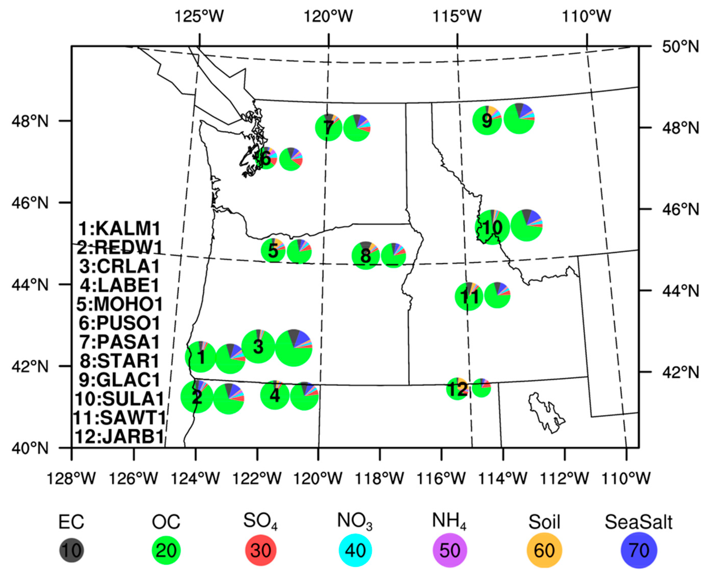
| Chemical composition | IMPROVE aerosol speciation | Hourly/in situ | Inter-agencies 4 |
| Data | Description | Source |
|---|---|---|
| Population | The USA Census Grids, 2010 [43] | NASA SEDAC 1 |
| Mortality | Multiple cause of deaths in August–December of 2017 | CDC WONDER 2 |
| Relative risk function for multiple-cause mortality | 0.11% (95% CI: 0, 0.26%) per 1 μg m−3 increase of surface PM2.5 concentration | Johnston et al. [1] |
| Metrics | CMAQ_SENS | CMAQ_MLR | CMAQ_RF | CMAQ_GBM |
|---|---|---|---|---|
| Area-weighted regional average (μg m−3) | 11.9 | 23.4 | 22.9 | 21.4 |
| Population-weighted regional average (μg m−3) | 4.5 | 15.9 | 12.8 | 10.9 |
| MAE (μg m−3) | 17.0 | 17.4 | 13.7 | 15.0 |
| FB (%) | −44% | −1% | 1% | −1% |
| R2 (unitless) | 0.42 | 0.45 | 0.59 | 0.54 |
| RMSE (μg m−3) | 36.1 | 33.8 | 28.8 | 30.3 |
© 2019 by the authors. Licensee MDPI, Basel, Switzerland. This article is an open access article distributed under the terms and conditions of the Creative Commons Attribution (CC BY) license (http://creativecommons.org/licenses/by/4.0/).
Share and Cite
Zou, Y.; O’Neill, S.M.; Larkin, N.K.; Alvarado, E.C.; Solomon, R.; Mass, C.; Liu, Y.; Odman, M.T.; Shen, H. Machine Learning-Based Integration of High-Resolution Wildfire Smoke Simulations and Observations for Regional Health Impact Assessment. Int. J. Environ. Res. Public Health 2019, 16, 2137. https://doi.org/10.3390/ijerph16122137
Zou Y, O’Neill SM, Larkin NK, Alvarado EC, Solomon R, Mass C, Liu Y, Odman MT, Shen H. Machine Learning-Based Integration of High-Resolution Wildfire Smoke Simulations and Observations for Regional Health Impact Assessment. International Journal of Environmental Research and Public Health. 2019; 16(12):2137. https://doi.org/10.3390/ijerph16122137
Chicago/Turabian StyleZou, Yufei, Susan M. O’Neill, Narasimhan K. Larkin, Ernesto C. Alvarado, Robert Solomon, Clifford Mass, Yang Liu, M. Talat Odman, and Huizhong Shen. 2019. "Machine Learning-Based Integration of High-Resolution Wildfire Smoke Simulations and Observations for Regional Health Impact Assessment" International Journal of Environmental Research and Public Health 16, no. 12: 2137. https://doi.org/10.3390/ijerph16122137
APA StyleZou, Y., O’Neill, S. M., Larkin, N. K., Alvarado, E. C., Solomon, R., Mass, C., Liu, Y., Odman, M. T., & Shen, H. (2019). Machine Learning-Based Integration of High-Resolution Wildfire Smoke Simulations and Observations for Regional Health Impact Assessment. International Journal of Environmental Research and Public Health, 16(12), 2137. https://doi.org/10.3390/ijerph16122137