
Evaluating Leaf and Canopy Reflectance of Stressed Rice Plants to Monitor Arsenic Contamination

Abstract
:
1. Introduction
2. Materials and Methods
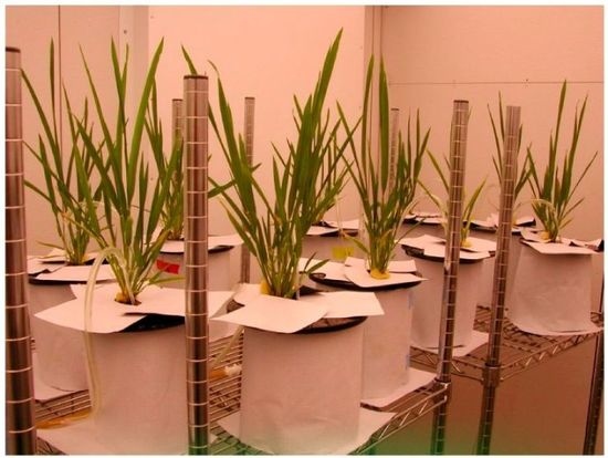
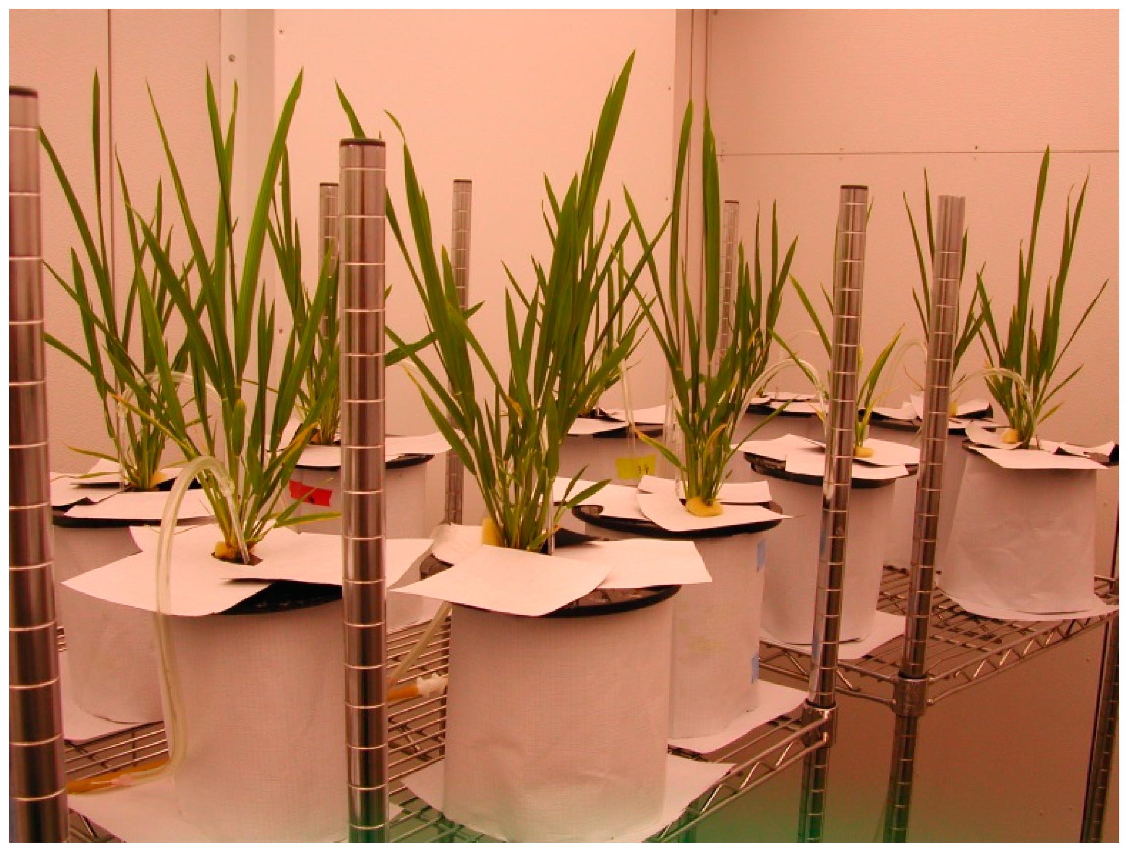
2.1. Hydroponic Growth Chamber Experiment
2.2. Measurement Procedures
2.2.1. Leaf Spectral Measurements
2.2.2. Bio-Physicochemical Measurements
2.2.3. Soil Reflectance Measurements
2.3. Simulated Canopy Reflectance
2.4. Vegetative Indices
2.5. Data Analyses
3. Results and Discussion
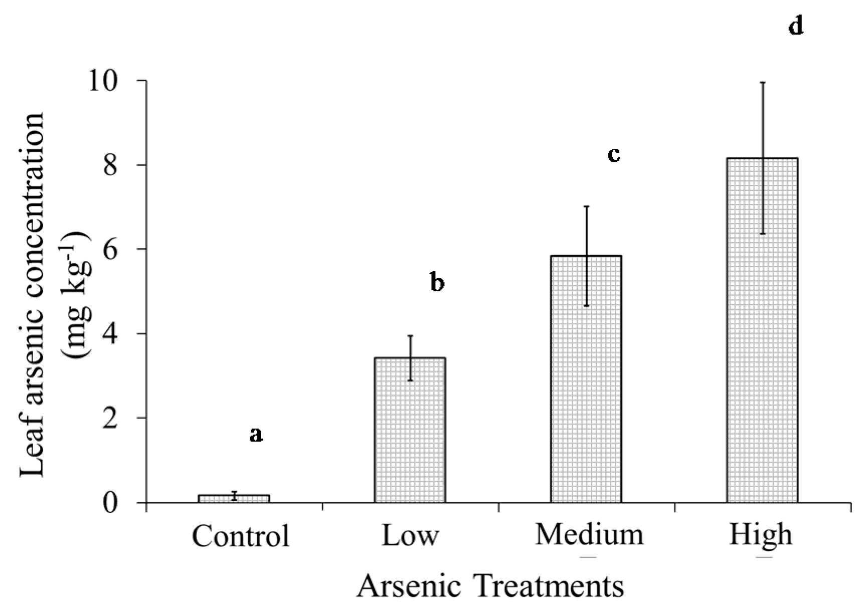
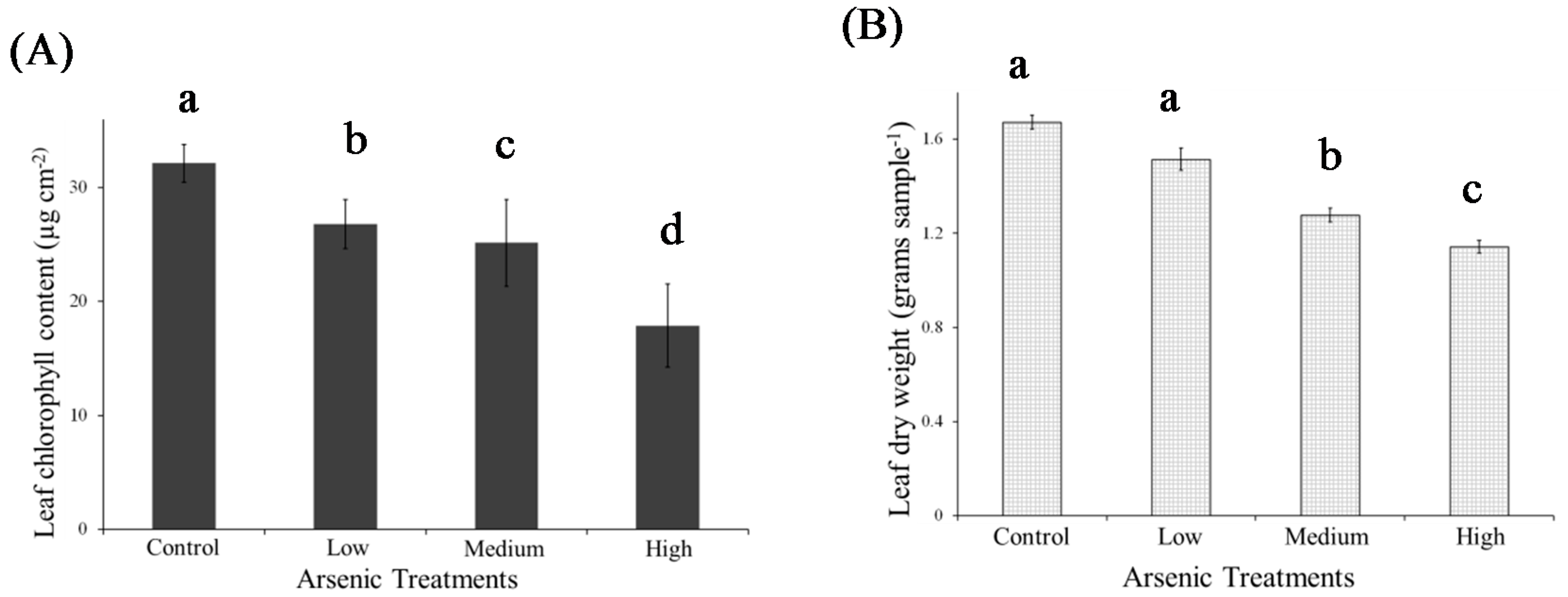
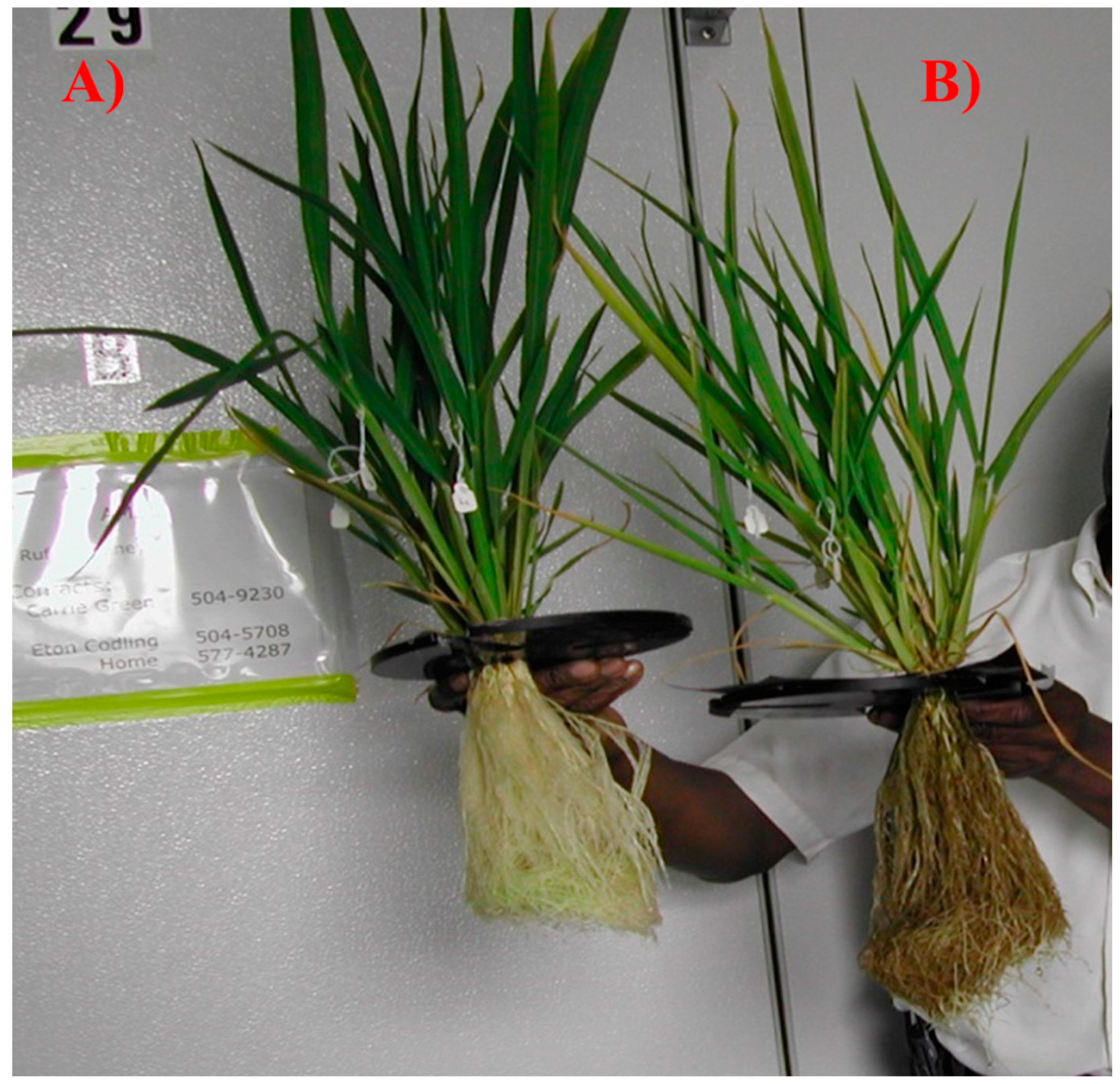
3.1. Plant as Uptake and Plant Stress
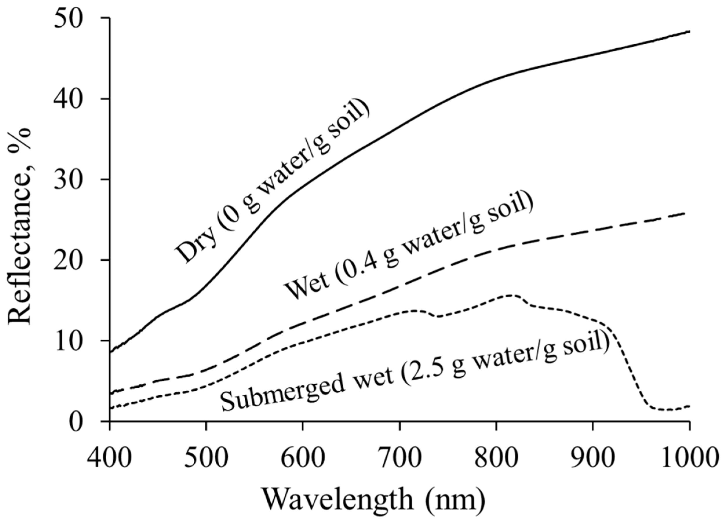
3.2. Soil Background Reflectance
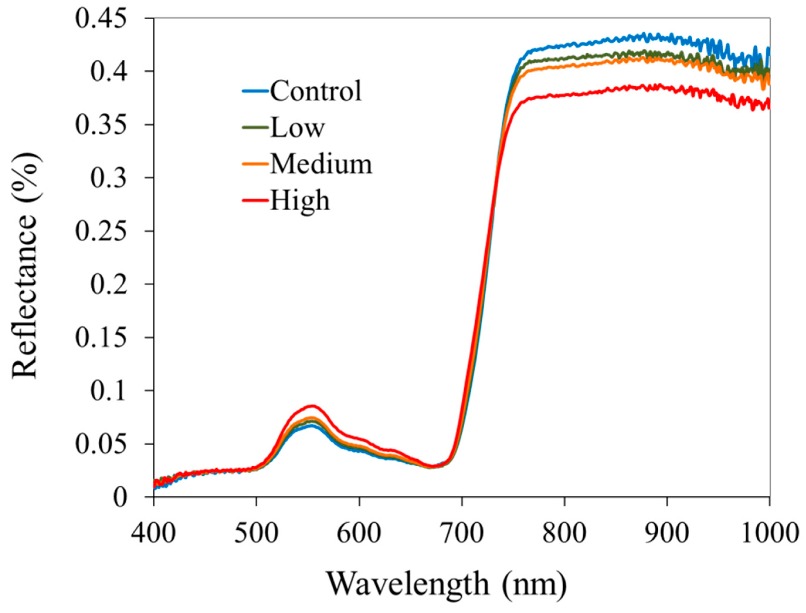
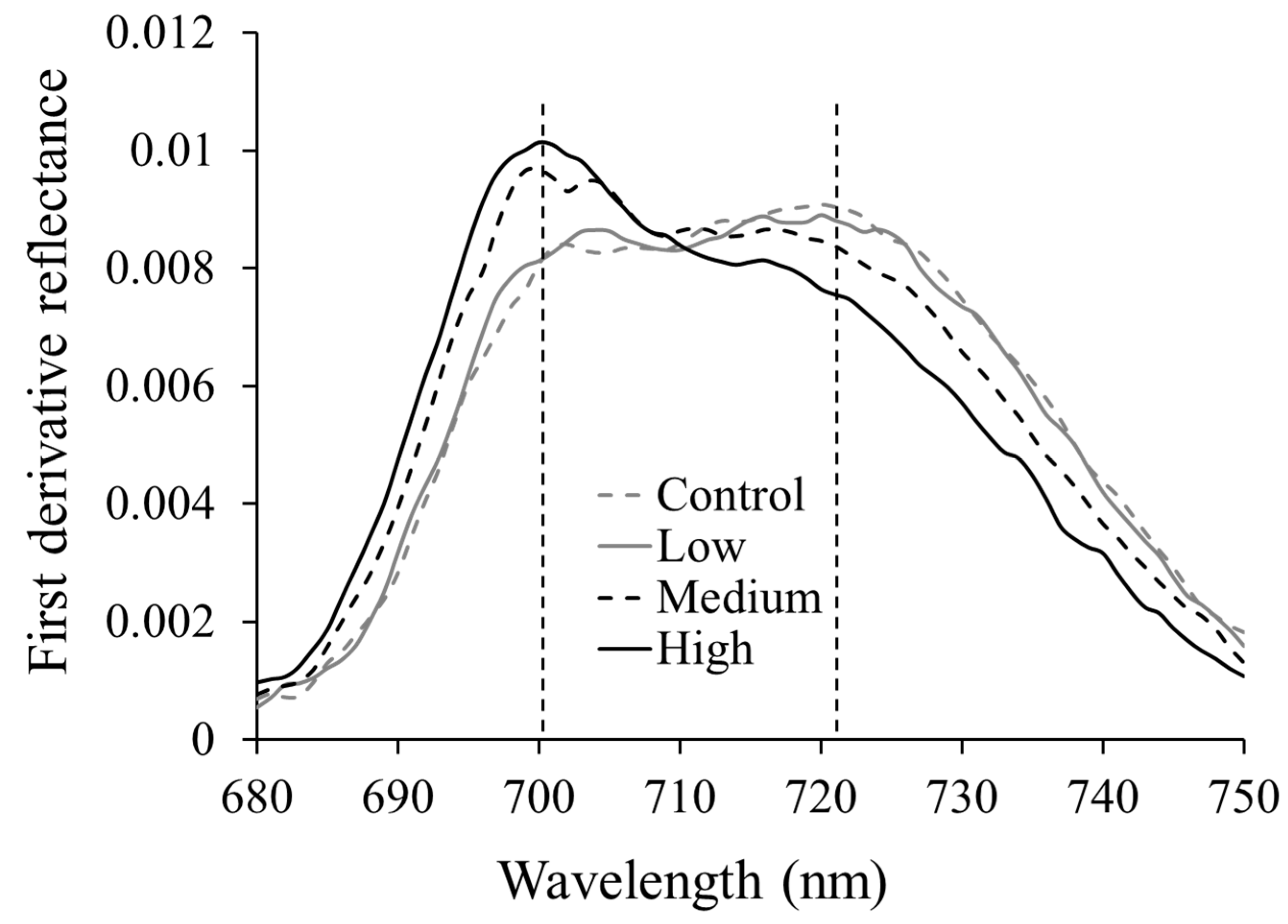
3.3. Leaf Reflectance and Derivative Reflectance
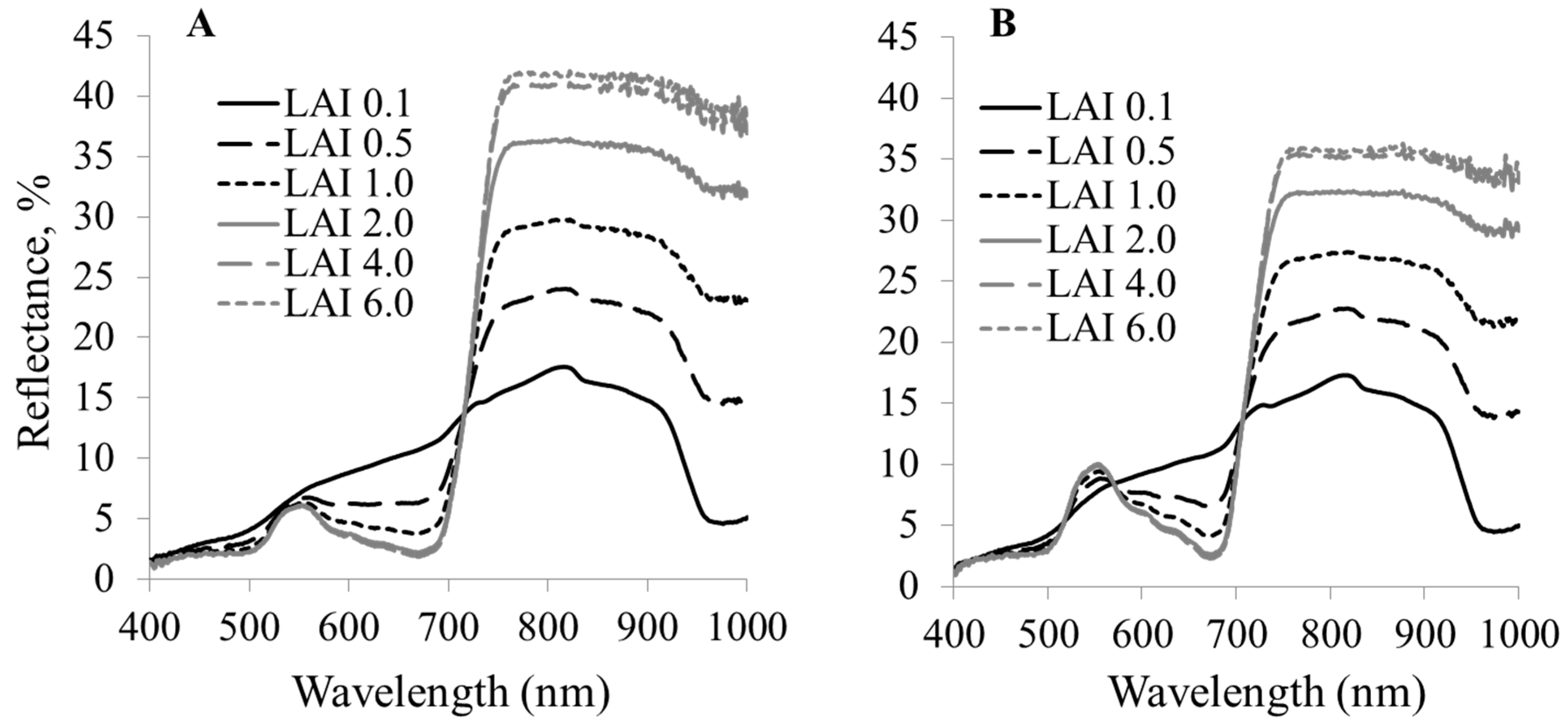
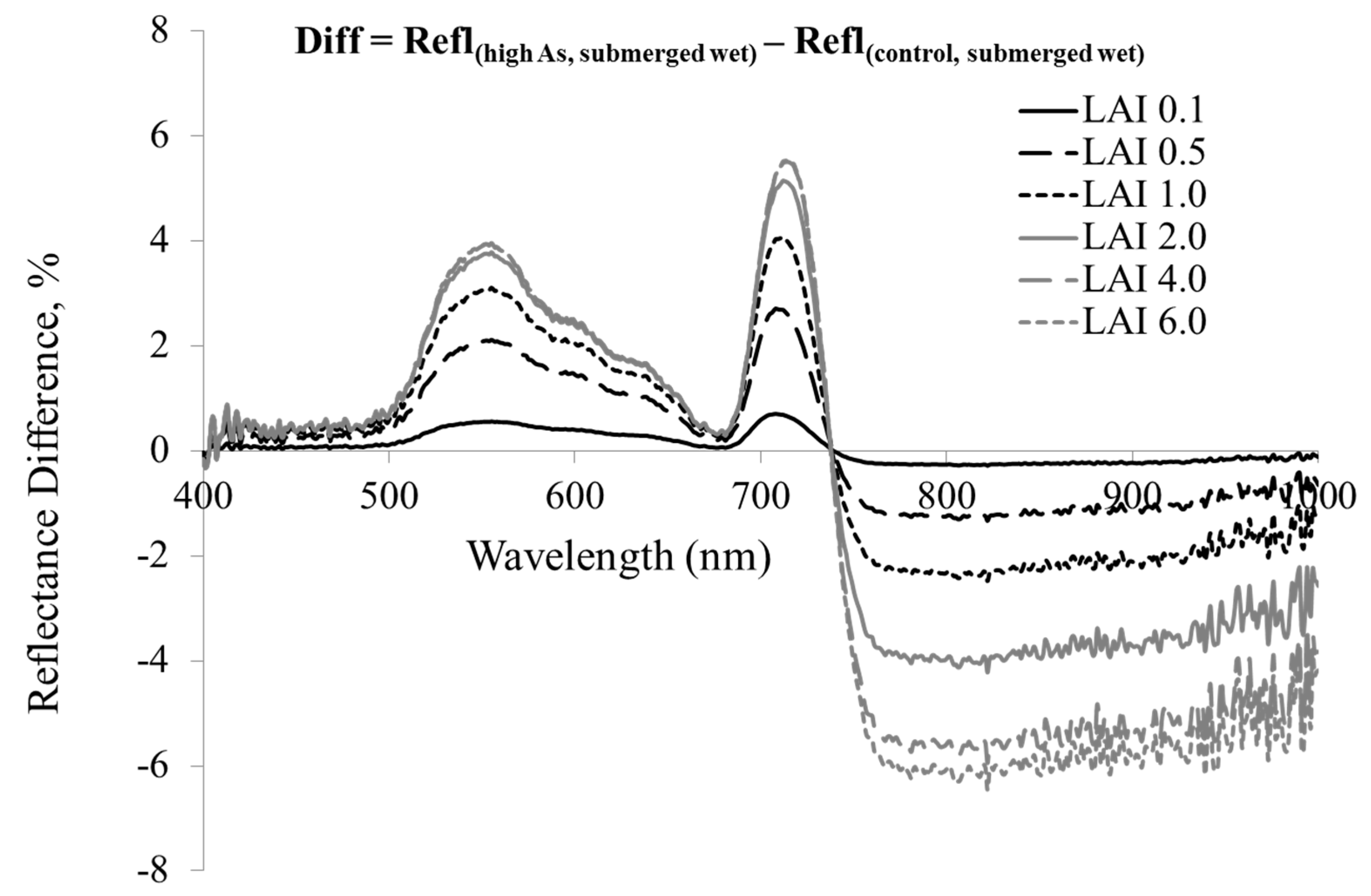
3.4. Canopy Reflectance
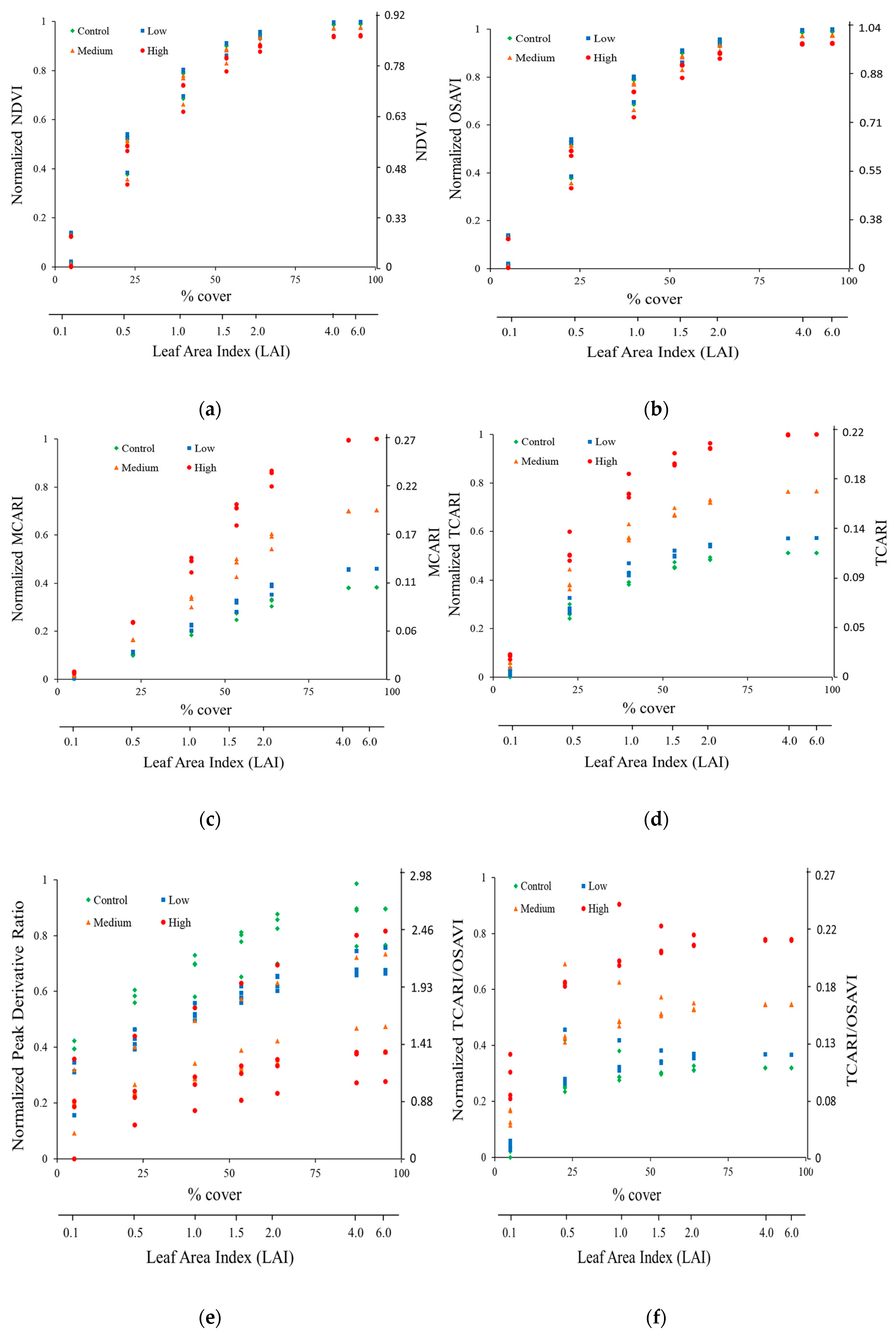
3.5. Relationship between Vegetative Indices and Plant as Levels at Leaf and Canopy Scale
3.5.1. Leaf Scale
3.5.2. Canopy Scale
4. Conclusions
Acknowledgments
Author Contributions
Conflicts of Interest
Abbreviations
| ARS | Agricultural Research Service |
| As | Arsenic |
| ICP-AES | Inductively Coupled Plasma Atomic Emission Spectrometry |
| LAI | Leaf Area Index |
| MCARI | Modified Chlorophyll Absorption Reflectance Index |
| NDVI | Normalized Difference Vegetative Index |
| NIR | Near Infrared |
| NIST | National Institute of Standards and Technology |
| OSAVI | Optimized soil adjusted vegetation index |
| PPFD | Photosynthetic Photon Flux Density |
| SAIL | Scattering by Arbitrarily Inclined Leaves |
| TCARI | Transformed chlorophyll absorption reflectance index |
| Vis | Vegetative Indices |
References
- Meharg, A.; Williams, P.; Adomako, E.; Lawgali, Y.; Deacon, C.; Villada, A.; Cambell, R.; Sun, G.; Zhu, Y.; Feldmann, J.; et al. Geographical variation in total and inorganic arsenic content of polished (white) rice. Environ. Sci. Technol. 2009, 43, 1612–1617. [Google Scholar] [CrossRef] [PubMed]
- Meharg, A.; Zhao, F.-J. Sources and losses of arsenic to paddy fields. In Arsenic & Rice; Springer: Dordrecht, The Netherlands, 2012; pp. 51–69. [Google Scholar]
- Syu, C.-H.; Huang, C.-C.; Jiang, P.-Y.; Lee, C.-H.; Lee, D.-Y. Arsenic accumulation and speciation in rice grains influenced by arsenic phytotoxicity and rice genotypes grown in arsenic-elevated paddy soils. J. Hazard. Mater. 2015, 286, 179–186. [Google Scholar] [CrossRef] [PubMed]
- Stoeva, N.; Bineva, T.Z. Oxidative changes and photosynthesis in oat plants grown in As-contaminated soil. Bulg. J. Plant Physiol. 2003, 29, 87–95. [Google Scholar]
- Ullrich-Eberius, C.; Sanz, A.; Novacky, A. Evaluation of arsenic and vandate–Associated changes of electrical membrane potential and phosphate transport in Lemna gibba. J. Exp. Bot. 1989, 40, 119–128. [Google Scholar] [CrossRef]
- Sohn, E. The toxic side of rice. Nature 2014, 514, S62–S63. [Google Scholar] [CrossRef] [PubMed]
- Meharg, A.A.; Rahman, M. Arsenic contamination of Bangladesh paddy field soils: Implications for rice contribution to arsenic consumption. Environ. Sci. Technol. 2003, 37, 229–234. [Google Scholar] [CrossRef] [PubMed]
- Abedin, M.J.; Feldmann, J.; Meharg, A.A. Uptake kinetics of arsenic species in rice plants. Plant Physiol. 2002, 128, 1120–1128. [Google Scholar] [CrossRef] [PubMed]
- Lin, S.C.; Chang, T.K.; Huang, W.D.; Lur, H.S.; Shyu, G.S. Accumulation of arsenic in rice plant: A study of an arsenic-contaminated site in Taiwan. Paddy Water Environ. 2015, 13, 11–18. [Google Scholar] [CrossRef]
- Roberts, L.C.; Hug, S.J.; Dittmar, J.; Voegelin, A.; Kretzschmar, R.; Wehrli, B.; Cirpka, O.A.; Saha, G.C.; Ashraf Ali, M.; Badruzzaman, A.B.M. Arsenic release from paddy soils during monsoon flooding. Nature Geosci. 2010, 3, 53–59. [Google Scholar] [CrossRef]
- Hossain, M.F. Arsenic contamination in Bangladesh—An overview. Agric. Ecosyst. Environ. 2006, 113, 1–16. [Google Scholar] [CrossRef]
- Abedin, M.J.; Cotter-Howells, J.; Meharg, A. Arsenic uptake and accumulation in rice (Oryza sativa L.) irrigated with contaminated water. Plant Soil 2002, 240, 311–319. [Google Scholar] [CrossRef]
- Brammer, H. Mitigation of arsenic contamination in irrigated paddy soils in south and South-East Asia. Environ. Int. 2009, 35, 856–863. [Google Scholar] [CrossRef] [PubMed]
- Li, R.Y.; Stroud, J.L.; Ma, J.F.; McGrath, S.P.; Zhao, F.J. Mitigation of arsenic accumulation in rice with water management and silicon fertilization. Environ. Sci. Technol. 2009, 43, 3778–3783. [Google Scholar] [CrossRef] [PubMed]
- Liu, W.; Zhu, Y.; Hu, Y.; Williams, P.; Gault, A.; Meharg, A.; Charnock, J.; Smith, F. Arsenic sequestration in iron plaque, its accumulation and speciation in mature rice plants (oryza sativa l.). Environ. Sci. Technol. 2006, 40, 5730–5736. [Google Scholar] [CrossRef] [PubMed]
- Xie, Z.; Huang, C. Control of arsenic toxicity in rice plants grown on an arsenic-polluted paddy soil. Commun. Soil Sci. Plant Anal. 1998, 29, 2471–2477. [Google Scholar] [CrossRef]
- Srivastava, P.; Singh, M.; Gupta, M.; Singh, N.; Kharwar, R.; Tripathi, R.; Nautiyal, C. Mapping of arsenic pollution with reference to paddy cultivation in the middle Indo-Gangetic plains. Environ. Monit. Assess. 2015, 187, 1–14. [Google Scholar] [CrossRef] [PubMed]
- Dittmar, J.; Voegelin, A.; Roberts, L.C.; Hug, S.J.; Saha, G.C.; Ali, M.A.; Badruzzaman, A.B.M.; Kretzschmar, R. Spatial distribution and temporal variability of arsenic in irrigated rice fields in Bangladesh. 2. Paddy soil. Environ. Sci. Technol. 2007, 41, 5967–5972. [Google Scholar] [CrossRef] [PubMed]
- Dat, J.; Vandenabeele, S.; Iranova, E.; Montagu, M.V.; Inze, D.; Breusegem, F.V. Dual action of the active oxygen species during plant stress responses. Cell. Mol. Life Sci. 2000, 57, 779–795. [Google Scholar] [CrossRef] [PubMed]
- Hartley-Whitaker, J.; Ainsworth, G.; Meharg, A. Copper and arsenic induced oxidative stress in Holcus lanatus L. clones with differential sensitivity. Plant Cell Environ. 2001, 24, 713–722. [Google Scholar] [CrossRef]
- Flora, S. Arsenic-induced oxidative stress and its reversibility following combined administration of N-acetylcysteine and meso 2, 3- dimercaptosuccinic acid in rats. Clin. Exp. Pharm. Physiol. 1999, 26, 865–869. [Google Scholar] [CrossRef]
- Choudhury, B.; Chowdhury, S.; Biswas, A. Regulation of growth and metabolism in rice (Oryza sativa L.) by arsenic and its possible reversal by phosphate. J. Plant Interact. 2011, 6, 15–24. [Google Scholar] [CrossRef]
- Rahman, M.; Hasegawa, H.; Rahman, M.; Islam, M.; Miah, M.; Tasmen, A. Effect of arsenic on photosynthesis, growth and yield of five widely cultivated rice (Oryza sativa L.) varieties in Bangladesh. Chemosphere 2007, 67, 1072–1079. [Google Scholar] [CrossRef] [PubMed]
- Shaibur, M.R.; Kitajima, N.; Sugawara, R.; Kondo, T.; Huq, S.M.I.; Kawai, S. Physiological and mineralogical properties of arsenic-induced chlorosis in rice seedlings grown hydroponically. Soil Sci. Plant Nutr. 2006, 52, 691–700. [Google Scholar] [CrossRef]
- Liu, M.; Liu, X.; Ding, W.; Wu, L. Monitoring stress levels on rice with heavy metal pollution from hyperspectral reflectance data using wavelet-fractal analysis. Int. J. Appl. Earth Obs. Geoinform. 2011, 13, 246–255. [Google Scholar] [CrossRef]
- Meggio, F.; Zarco-Tejada, P.; Nunez, L.; Sepulcre-Canto, G.; Gonzalez, M.; Martin, P. Grape quality assessment in vineyards affected by iron deficiency chlorosis using narrow-band physiological remote sensing indices. Remote Sens. Environ. 2010, 114, 1968–1986. [Google Scholar] [CrossRef]
- Bandaru, V.; Hansen, D.J.; Codling, E.E.; Daughtry, C.S.; White-Hansen, S.; Green, C.E. Quantifying arsenic-induced morphological changes in spinach leaves: Implications for remote sensing. Int. J. Remote Sens. 2010, 31, 4163–4177. [Google Scholar] [CrossRef]
- Yang, C.-M.; Cheng, C.-H.; Chen, R.-K. Changes in spectral characteristics of rice canopy infested with brown planthopper and leaffolder. Crop Sci. 2007. [Google Scholar] [CrossRef]
- Carter, G.A.; Knapp, A.K. Leaf optical properties in higher plants: Linking spectral characteristics to stress and chlorophyll concentration. Am. J. Bot. 2001, 88, 677–684. [Google Scholar] [CrossRef] [PubMed]
- Shi, T.; Liu, H.; Wang, J.; Chen, Y.; Fei, T.; Wu, G. Monitoring arsenic contamination in agricultural soils with reflectance spectroscopy of rice plants. Environ. Sci. Technol. 2014, 48, 6264–6272. [Google Scholar] [CrossRef] [PubMed]
- Daughtry, C.S.T.; Walthall, C.L.; Kim, M.S.; de Colstoun, E.B.; McMurtrey, J.E., III. Estimating corn leaf chlorophyll concentration from leaf and canopy reflectance. Remote Sens. Environ. 2000, 74, 229–239. [Google Scholar] [CrossRef]
- Eitel, J.; Long, D.; Gessler, P.; Hunt, E. Combined spectral index to improve ground-based estimates of nitrogen status in dryland wheat. Agron. J. 2008, 100, 1694–1702. [Google Scholar] [CrossRef]
- Kukier, U.; Chaney, R.L. Growing rice grain with controlled cadmium concentrations. J. Plant Nutr. 2002, 25, 1793–1820. [Google Scholar] [CrossRef]
- Analytical Spectral Devices. FieldSpec Users Guide; Analytical Spectral Devices: Boulder, CO, USA, 1997. [Google Scholar]
- Wellburn, A.R. The spectral determination of chlorophylls a and b, as well as total carotenoids, using various solvents with spectrophotometers of different resolution. J. Plant Physiol. 1994, 144, 307–313. [Google Scholar] [CrossRef]
- Codling, E.E.; Ritchie, J.C. Eastern gama grass uptake of lead and arsenic from lead arsenate contaminated soil amended with lime and phosphorus. Soil Sci. 2005, 170, 413–424. [Google Scholar] [CrossRef]
- Walter-Shea, E.A.; Biehl, L.L. Measuring vegetation spectral properties. Remote Sens. Rev. 1990, 5, 179–205. [Google Scholar] [CrossRef]
- Haboudane, D.; Miller, J.; Tremblay, N.; Zarco-Tejada, P.; Dextraze, L. Integrated narrow-band vegetation indices for prediction of crop chlorophyll content for application to precision agriculture. Remote Sens. Environ. 2002, 81, 416–426. [Google Scholar] [CrossRef]
- Hunt, E.; Doraiswamy, P.; McMurtrey, J.; Daughtry, C.; Perry, E.; Akhmedov, B. A visible band index for remote sensing leaf Chlorophyll content at the Canopy Scale. Int. J. Appl. Earth Obs. Geoinform. 2013, 21, 103–112. [Google Scholar] [CrossRef]
- Chen, P.; Haboudane, D.; Tremblay, N.; Wang, J.; Vigneault, P.; Li, B. New spectral indicator assessing the efficiency of crop nitrogen treatment in corn and wheat. Remote Sens. Environ. 2010, 114, 1987–1997. [Google Scholar] [CrossRef]
- Li, F.; Miao, Y.; Hennig, S.; Gnyp, M.; Chen, X.; Jia, L.; Bareth, G. Evaluating hyperspectral vegetation indices for estimating nitrogen concentration of winter wheat at different growth stages. Precis. Agric. 2010, 11, 335–357. [Google Scholar] [CrossRef]
- Hansen, P.; Schjoerring, J. Reflectance measurement of canopy biomass and nitrogen status in wheat crops using normalized difference vegetation indices and partial least squares regression. Remote Sens. Environ. 2003, 86, 542–553. [Google Scholar] [CrossRef]
- Penuelas, J.; Gamon, J.; Fredeen, A.; Merino, J.; Field, C. Reflectance indexes associated with physiological-changes in nitrogen-limited and water-limited sunflower leaves. Remote Sens. Environ. 1994, 48, 135–146. [Google Scholar] [CrossRef]
- Hunt, E.; Daughtry, C.; Eitel, J.; Long, D. Remote sensing leaf chlorophyll content using a visible band index. Agron. J. 2011, 103, 1090–1099. [Google Scholar] [CrossRef]
- Smith, K.L.; Steven, M.D.; Colls, J.J. Use of hyperspectral derivative ratios in the red-edge region to identify plant stress responses to gas leaks. Remote Sens. Environ. 2004, 92, 207–217. [Google Scholar] [CrossRef]
- Rouse, J.W.; Hass, R.H.; Schell, J.A.; Deering, D.W.; Harlan, J.C. Monitoring the Vernal Advancement and Retrogradation (Greenwave Effect) of Natural Vegetation NASA/GSFC Type III Final Report; GSFC: Greenbelt, MD, USA, 1974. [Google Scholar]
- Rondeaux, G.; Steven, M.; Baret, F. Optimization of soil-adjusted vegetation indices. Remote Sens. Environ. 1996, 55, 95–107. [Google Scholar] [CrossRef]
- SAS Institute Inc. SAS; SAS Institute Inc.: Cary, NC, USA, 2002. [Google Scholar]
- Lobell, D.B.; Asner, G.P. Moisture effects on soil reflectance. Soil Sci. Soc. Am. J. 2002, 66. [Google Scholar] [CrossRef]
- Horler, D.N.H.; Barber, J.; Baringer, A.R. Effects of heavy metals on the absorbance and reflectance spectra of plants. Int. J. Remote Sens. 1980, 1, 121–136. [Google Scholar] [CrossRef]
- Sridhar, B.B.M.; Han, F.X.; Diehl, S.V.; Monts, D.L.; Su, Y. Spectral reflectance and leaf internal structure changes of barley plants due to phytoextraction of zinc and cadmium. Int. J. Remote Sens. 2007, 28, 1041–1054. [Google Scholar] [CrossRef]
- Slonecker, T.; Haack, B.; Price, S. Spectroscopic analysis of arsenic uptake in Pteris ferns. Remote Sens. 2009, 1, 644–675. [Google Scholar] [CrossRef]
- Horler, D.N.H.; Dockray, M.; Barber, J.; Barringer, A.R. Red edge measurements for remote sensing plant chlorophyll content. Adv. Space Res. 1983, 3, 273–277. [Google Scholar] [CrossRef]
- Perry, E.M.; Roberts, D.A. Sensitivity of narrow-band and broad-band indices for assessing nitrogen availability and water stress in an annual crop. Agron. J. 2008, 100. [Google Scholar] [CrossRef]
- Tajeda, P.J.Z.; Berjon, A.; Miller, J.R. Stress detection in crops with hyperspectral remote sensing and physical simulation models. In Proceedings of the Airborne Imaging Spectroscopy Workshop, Bruges, Belgium, 8 October 2004.


| Compound | Concentration |
|---|---|
| (mM) | |
| CaCl2 | 0.5 |
| KNO3 | 2.0 |
| MgSO4 | 0.5 |
| (NH4)2SO4 | 0.5 |
| (µM) | |
| FeEDTA | 10.0 |
| Na2MoO4 | 0.1 |
| H3BO3 | 20.0 |
| MnCl2 | 1.0 |
| CuSO4 | 2.0 |
| ZnSO4 | 2.0 |
| Parameter | Values |
|---|---|
| Leaf reflectance and transmittance | Four arsenic levels (i.e., control, low, medium and high) |
| Soil reflectance | DeWitt silt loam soil (dry, wet, submerged) |
| Leaf area index (LAI) | 0.1, 0.5, 1.0, 1.5, 2.0, 4.0, 6.0 |
| Leaf angle distribution | Erectophile |
| View zenith angle | 0 degrees (nadir) |
| Sun zenith angle | 45 degrees |
| Fraction of direct incoming radiation | 1.0 |
| Type | Name | Abbrev. | Equation | Reference |
|---|---|---|---|---|
| Red-NIR † | Normalized difference vegetation index | NDVI | (Rn − Rr)/(Rn + Rr) | [46] |
| Red-NIR | Optimized soil adjusted vegetation index | OSAVI | (Rn − Rr)/Rn + Rr + 0.16) | [47] |
| Red-RE ‡ | Modified chlorophyll absorption reflectance index | MCARI | [(Re − Rr) − 0.2(Re − Rg)](Re/Rr) | [31] |
| Red-RE | Transformed chlorophyll absorption reflectance index | TCARI | 3[(Rre − Rr) − 0.2(Re − Rg)(Re/Rr)] | [48] |
| RE | Peaks derivative ratio | PDR | Der.720/Der.700 | [45] |
| Combined indices | TCARI/OSAVI | - | TCARI/OSAVI | [48] |
| Spectral Index | Slope | Intercept | r2 | RMSE |
|---|---|---|---|---|
| NDVI | −316.6 | 278.7 | 0.69 | 1.99 |
| OSAVI | −74.9 | 44.1 | 0.73 | 1.84 |
| MCARI | 143.3 | −8.6 | 0.85 | 1.23 |
| TCARI | 580.2 | −31.6 | 0.88 | 1.10 |
| PDR | −20.5 | 24.5 | 0.79 | 1.45 |
| TCARI/OSAVI | 163.2 | −14.8 | 0.89 | 1.11 |
| Source of Variation | ||||||
|---|---|---|---|---|---|---|
| Spectral Variable | Background | Arsenic Concentration | LAI | BGxLAI | BGxArsenic | LAIxArsenic |
| NDVI | 1.4 | 0.8 | 97.5 | 0.3 | − | − |
| OSAVI | 1.3 | 0.8 | 97.5 | 0.3 | − | − |
| GNDVI | 4.6 | 14.9 | 76.9 | 2.73 | 0.5 | 0.2 |
| MCARI | 0.1 | 45.4 | 51.9 | − | − | 2.5 |
| TCARI | 0.2 | 43.8 | 54.8 | − | − | 1.1 |
| Peak Derivative Ratio | 16.4 | 44.2 | 30.9 | 0.43 | 3.6 | 0.6 |
| TCARI/OSAVI | 2.6 | 74.1 | 22.2 | 0.63 | 0.2 | 0.3 |
| Degrees of freedom | 3 | 3 | 6 | 18 | 9 | 18 |
© 2016 by the authors; licensee MDPI, Basel, Switzerland. This article is an open access article distributed under the terms and conditions of the Creative Commons Attribution (CC-BY) license (http://creativecommons.org/licenses/by/4.0/).
Share and Cite
Bandaru, V.; Daughtry, C.S.; Codling, E.E.; Hansen, D.J.; White-Hansen, S.; Green, C.E. Evaluating Leaf and Canopy Reflectance of Stressed Rice Plants to Monitor Arsenic Contamination. Int. J. Environ. Res. Public Health 2016, 13, 606. https://doi.org/10.3390/ijerph13060606
Bandaru V, Daughtry CS, Codling EE, Hansen DJ, White-Hansen S, Green CE. Evaluating Leaf and Canopy Reflectance of Stressed Rice Plants to Monitor Arsenic Contamination. International Journal of Environmental Research and Public Health. 2016; 13(6):606. https://doi.org/10.3390/ijerph13060606
Chicago/Turabian StyleBandaru, Varaprasad, Craig S. Daughtry, Eton E. Codling, David J. Hansen, Susan White-Hansen, and Carrie E. Green. 2016. "Evaluating Leaf and Canopy Reflectance of Stressed Rice Plants to Monitor Arsenic Contamination" International Journal of Environmental Research and Public Health 13, no. 6: 606. https://doi.org/10.3390/ijerph13060606
APA StyleBandaru, V., Daughtry, C. S., Codling, E. E., Hansen, D. J., White-Hansen, S., & Green, C. E. (2016). Evaluating Leaf and Canopy Reflectance of Stressed Rice Plants to Monitor Arsenic Contamination. International Journal of Environmental Research and Public Health, 13(6), 606. https://doi.org/10.3390/ijerph13060606