
A Combination of Geographically Weighted Regression, Particle Swarm Optimization and Support Vector Machine for Landslide Susceptibility Mapping: A Case Study at Wanzhou in the Three Gorges Area, China


Abstract
:1. Introduction
2. Related Techniques
2.1. Geographically Weighted Regression
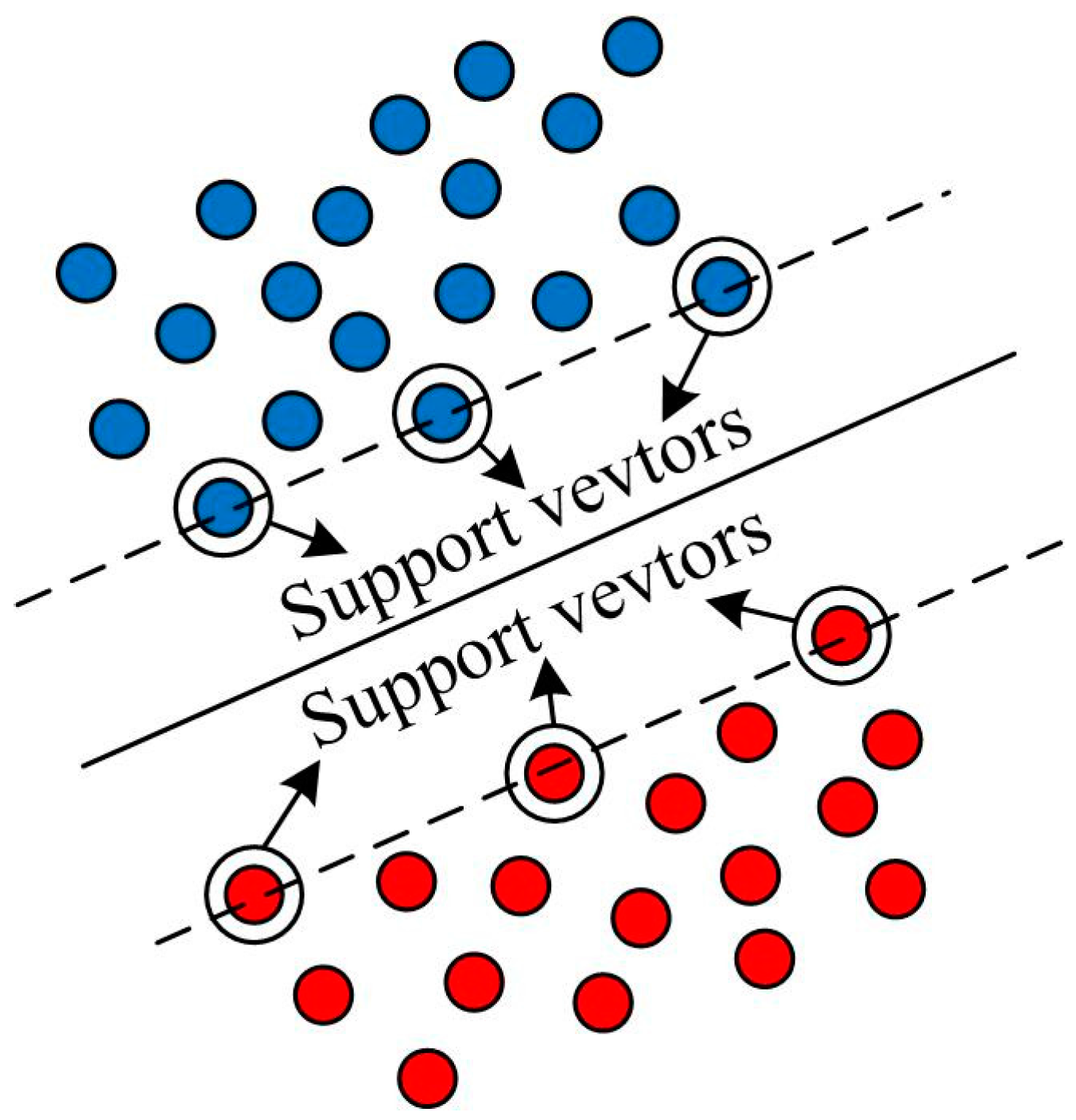
2.2. Support Vector Machine
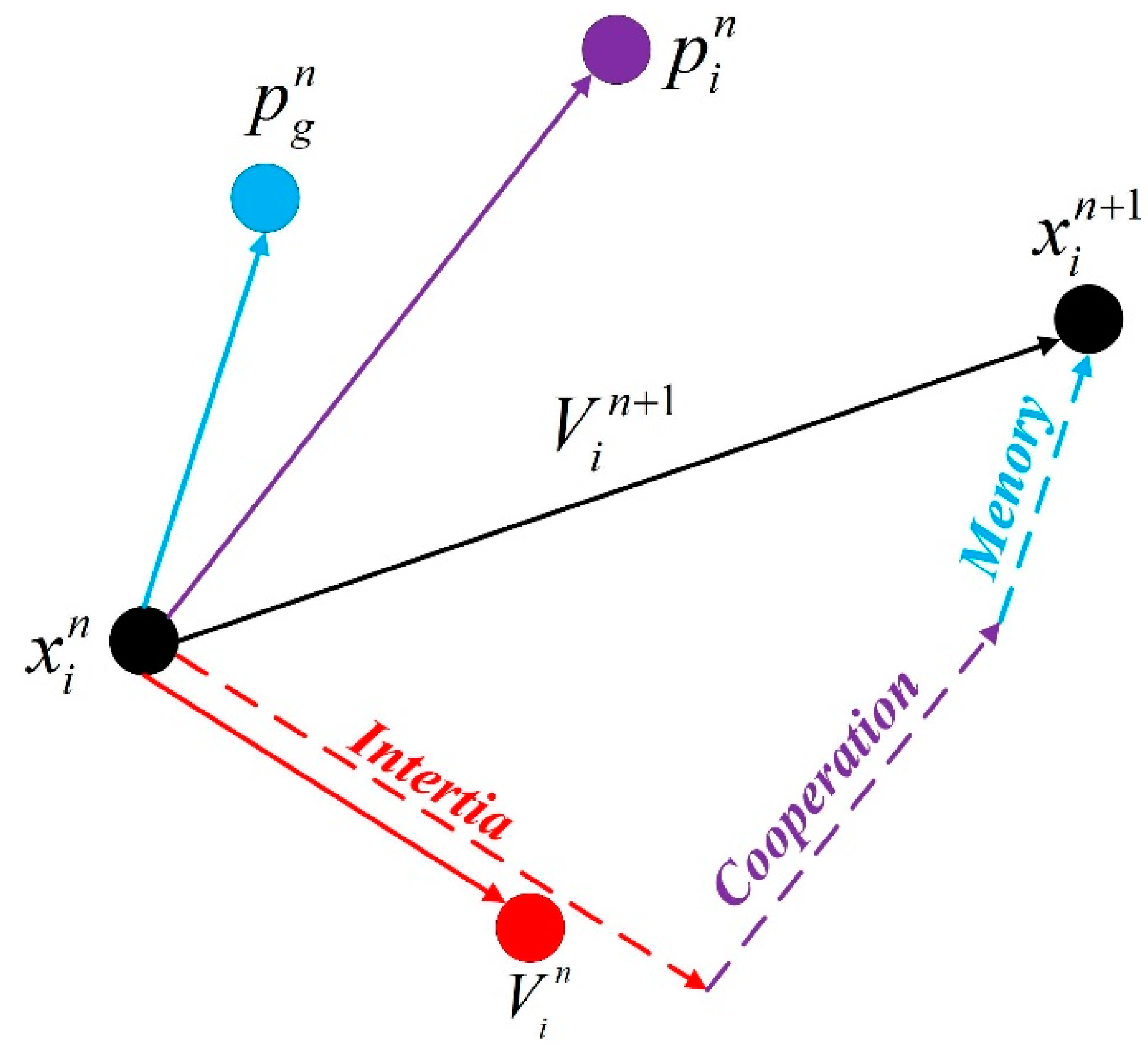
2.3. Particle Swarm Optimization
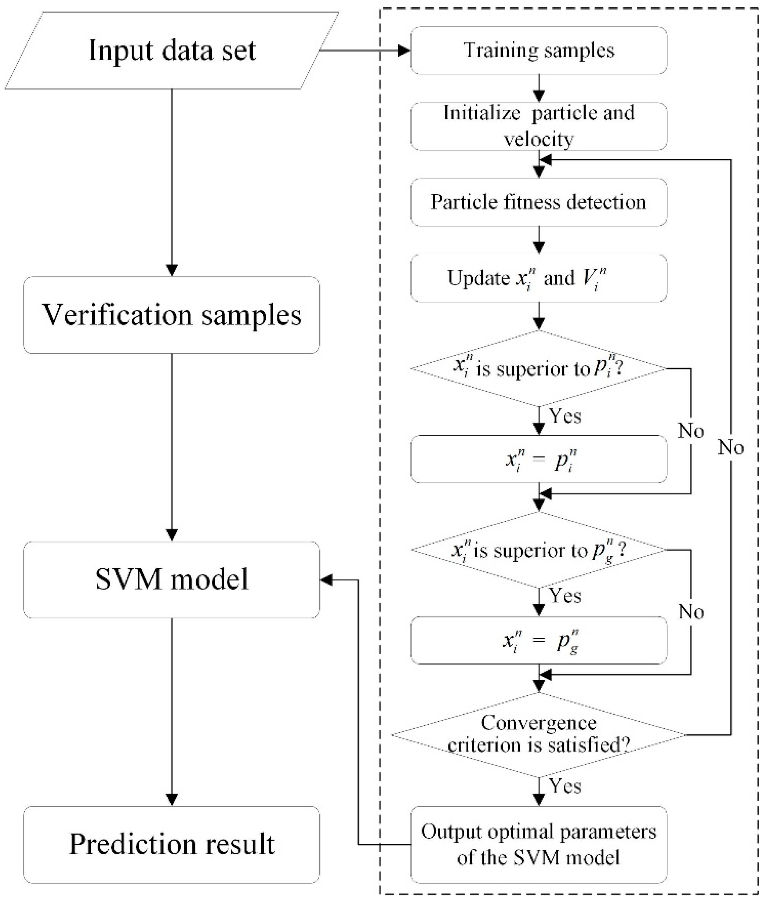
2.4. The PSO-SVM Model
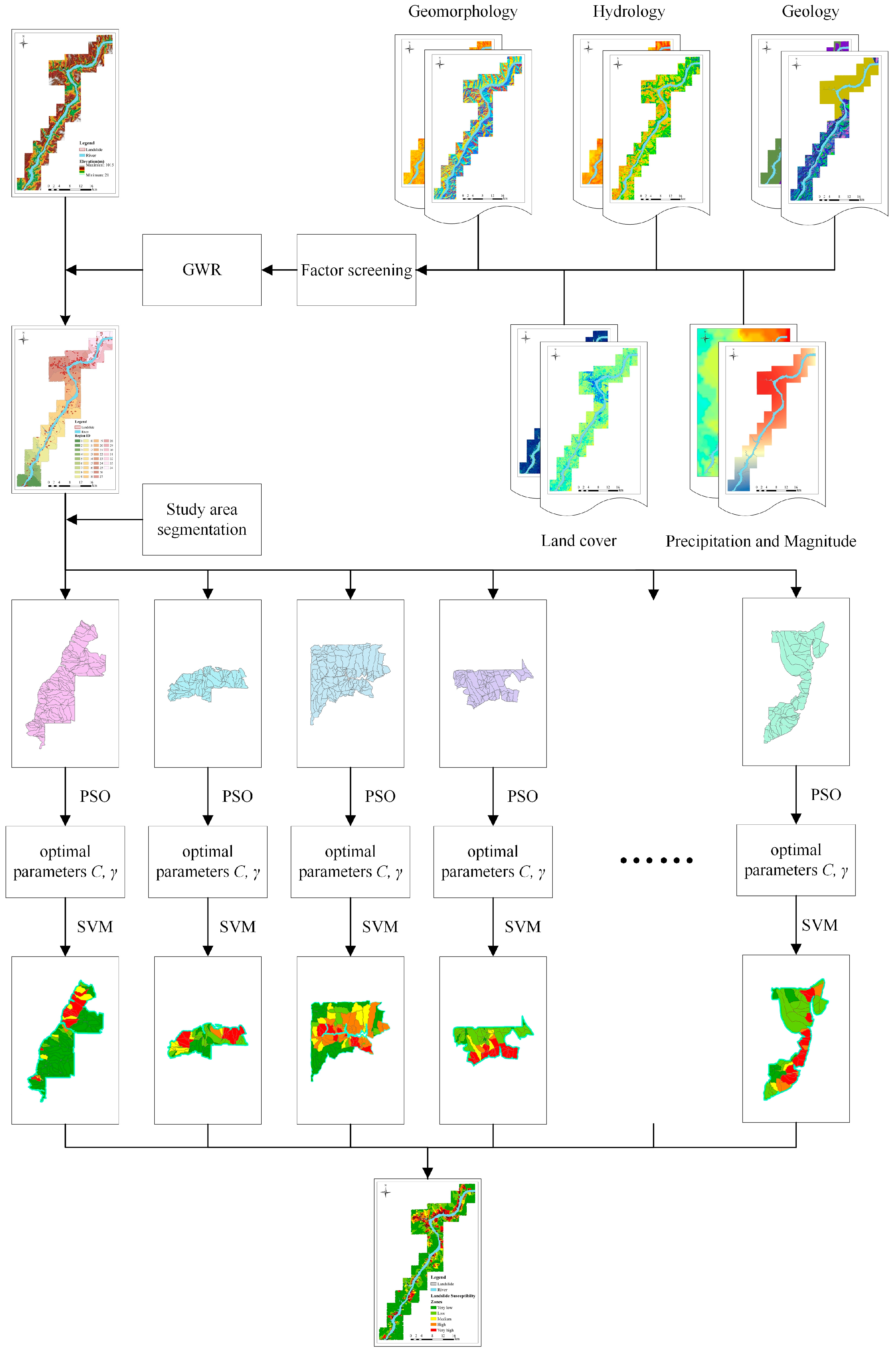
3. The Proposed GWR-PSO-SVM Model
3.1. Factor Screening
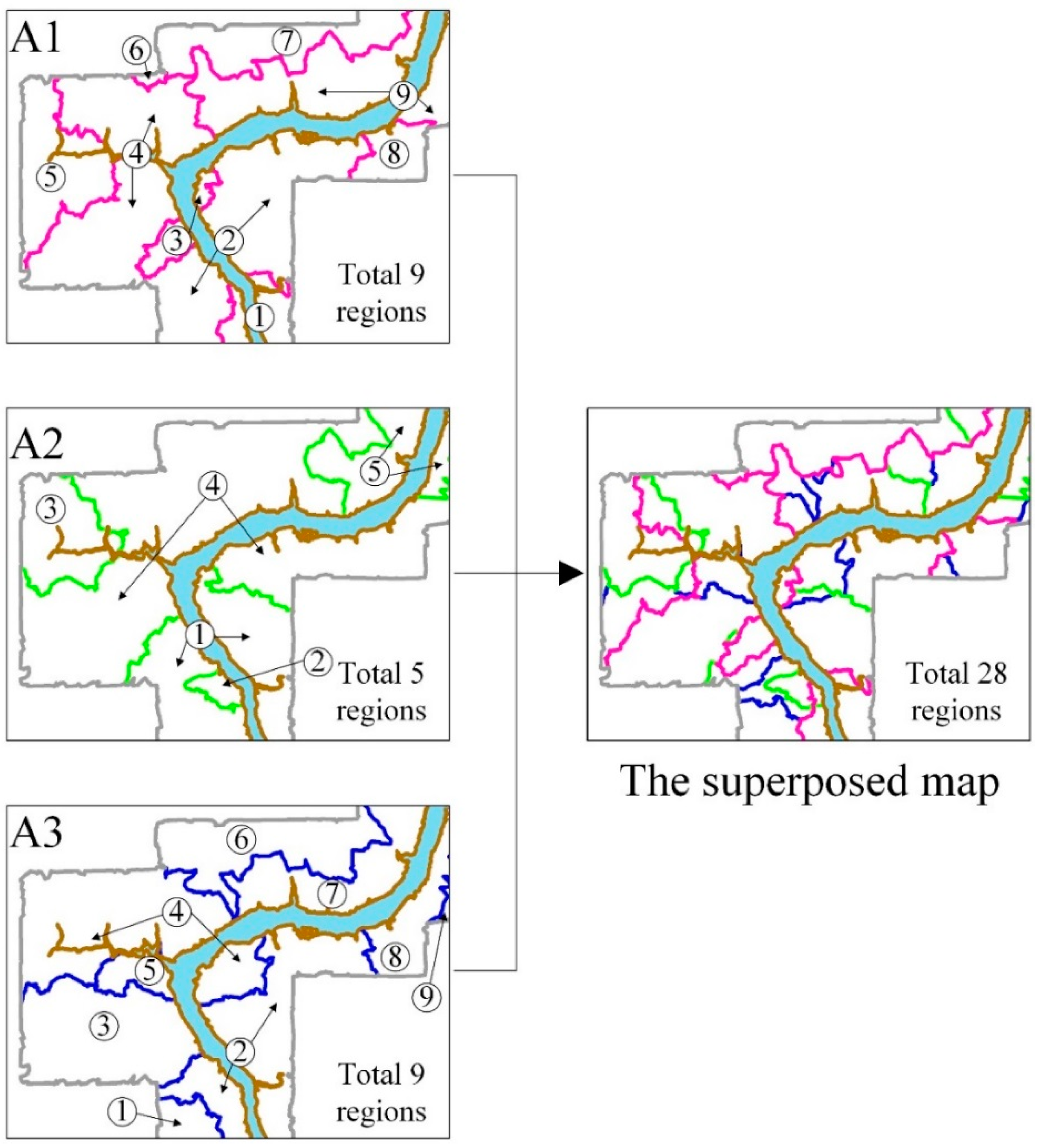
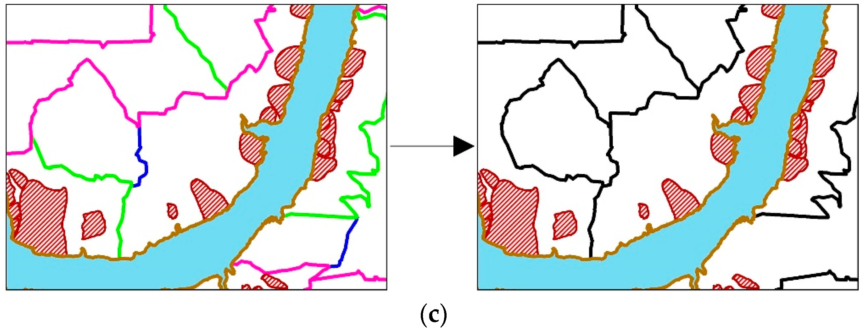
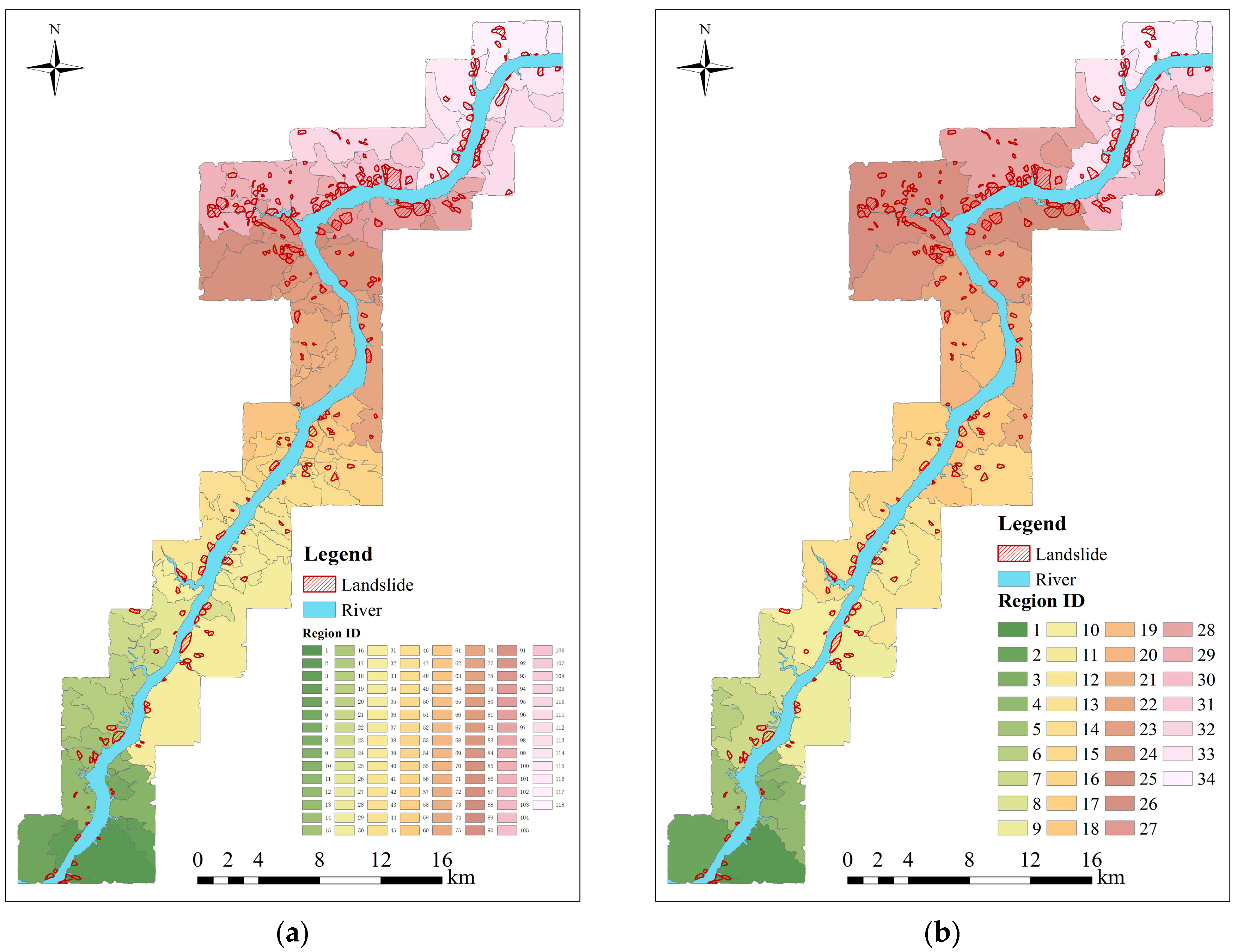
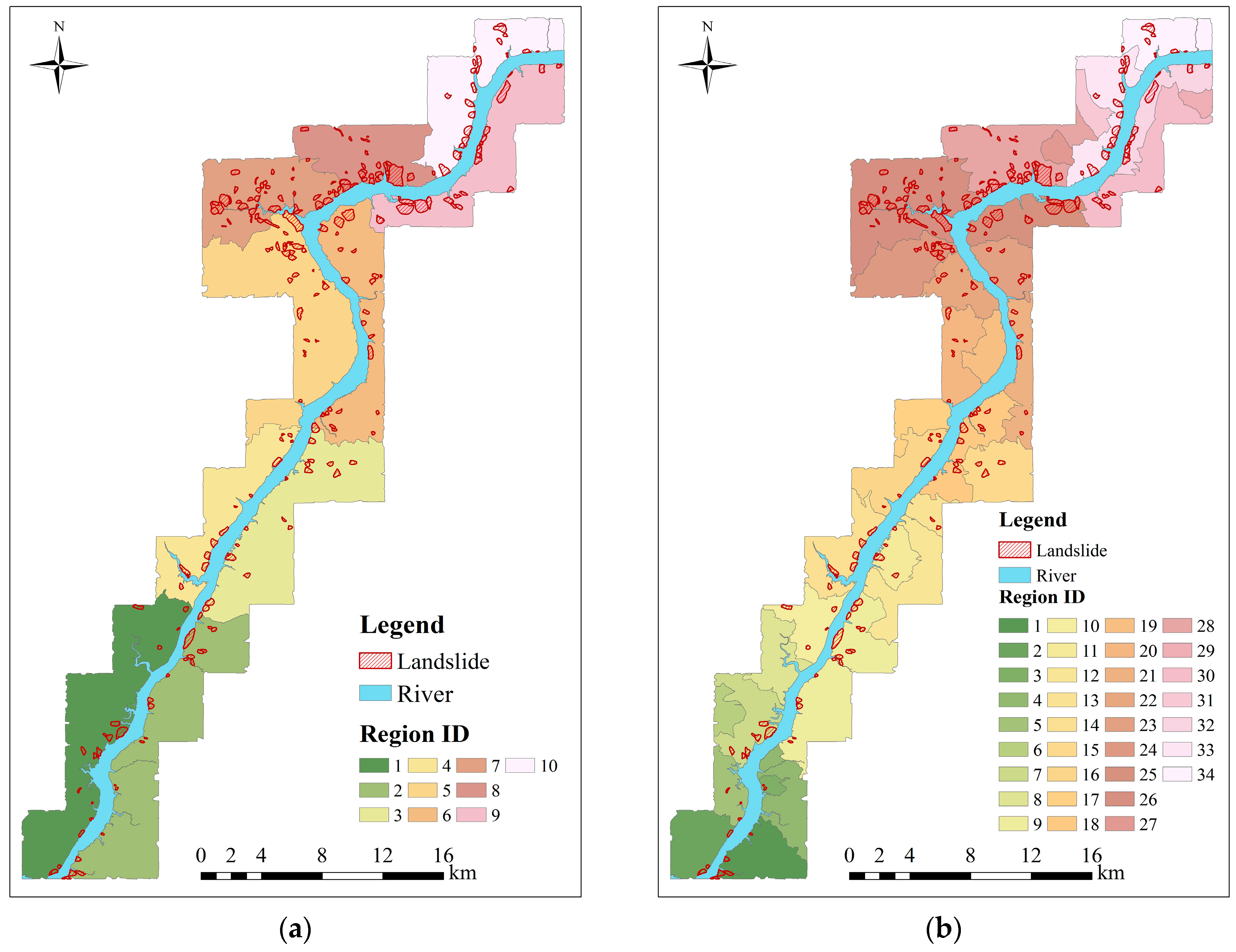
3.2. Study Area Segmentation
3.3. The GWR-PSO-SVM Model
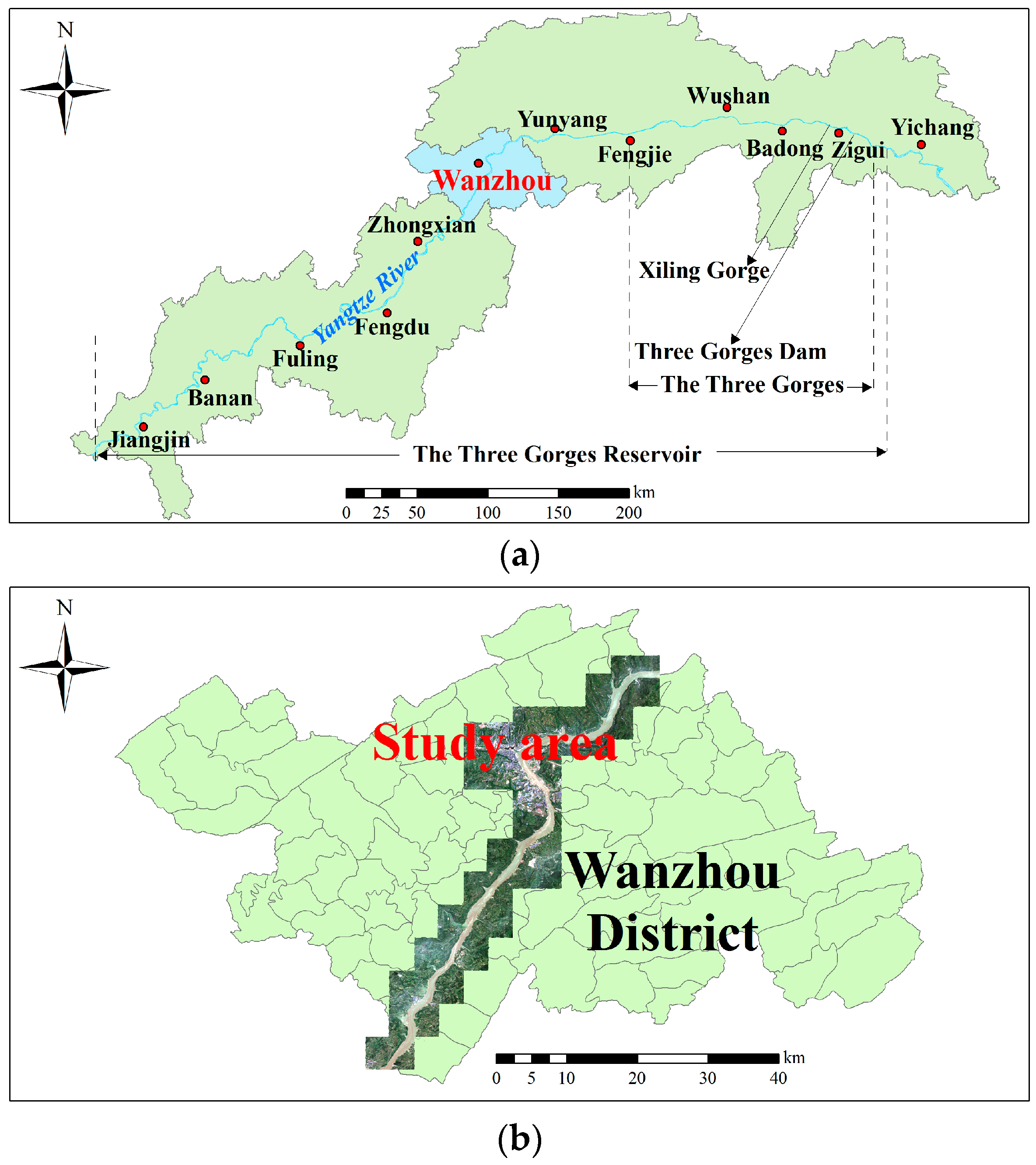
4. Study Area and Data
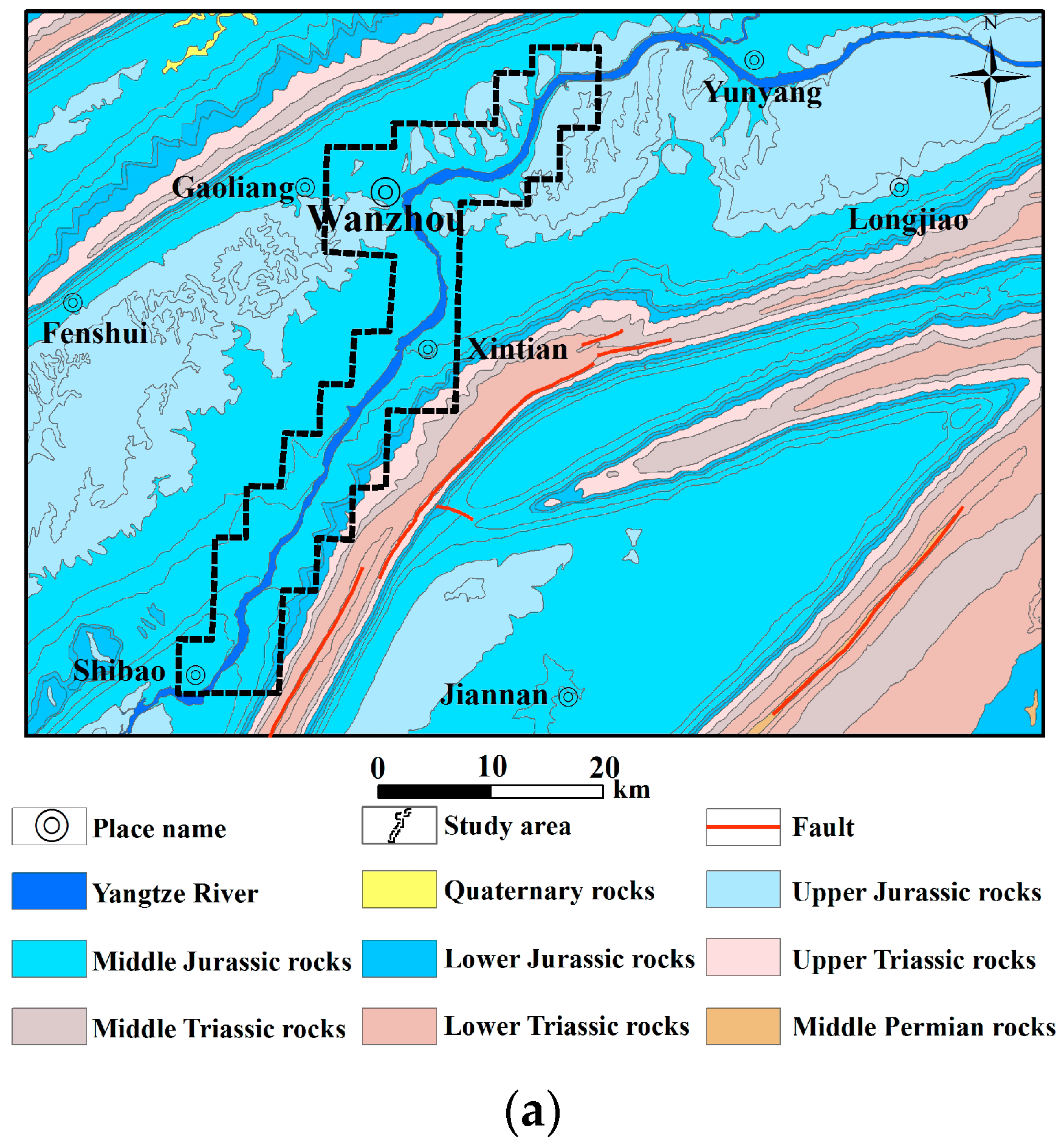
4.1. General Characteristics
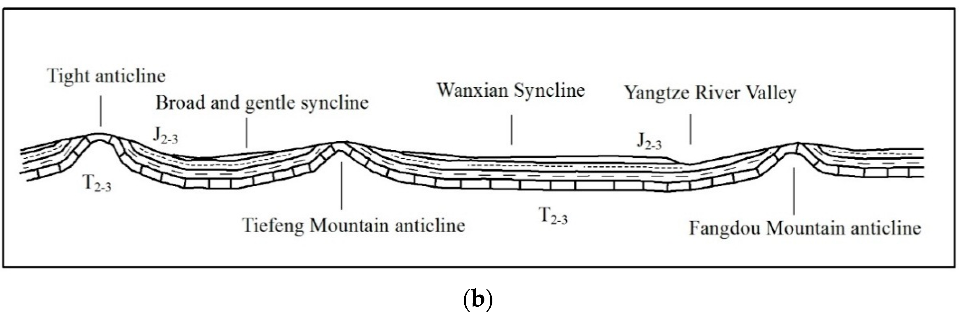
4.2. Geological Setting
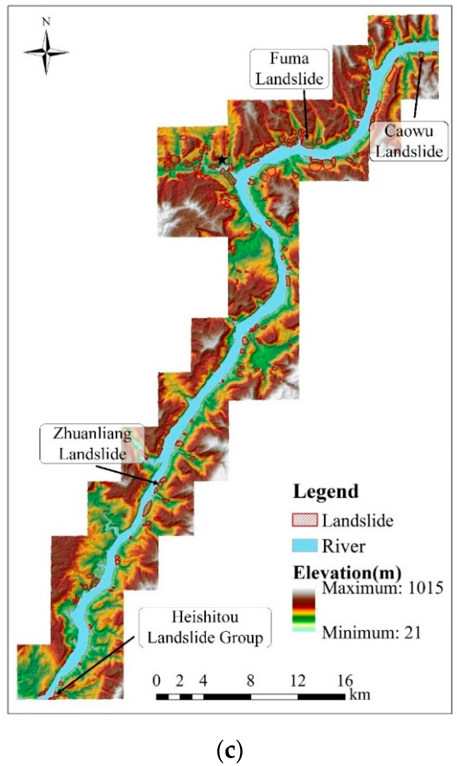
4.3. Description of Landslides
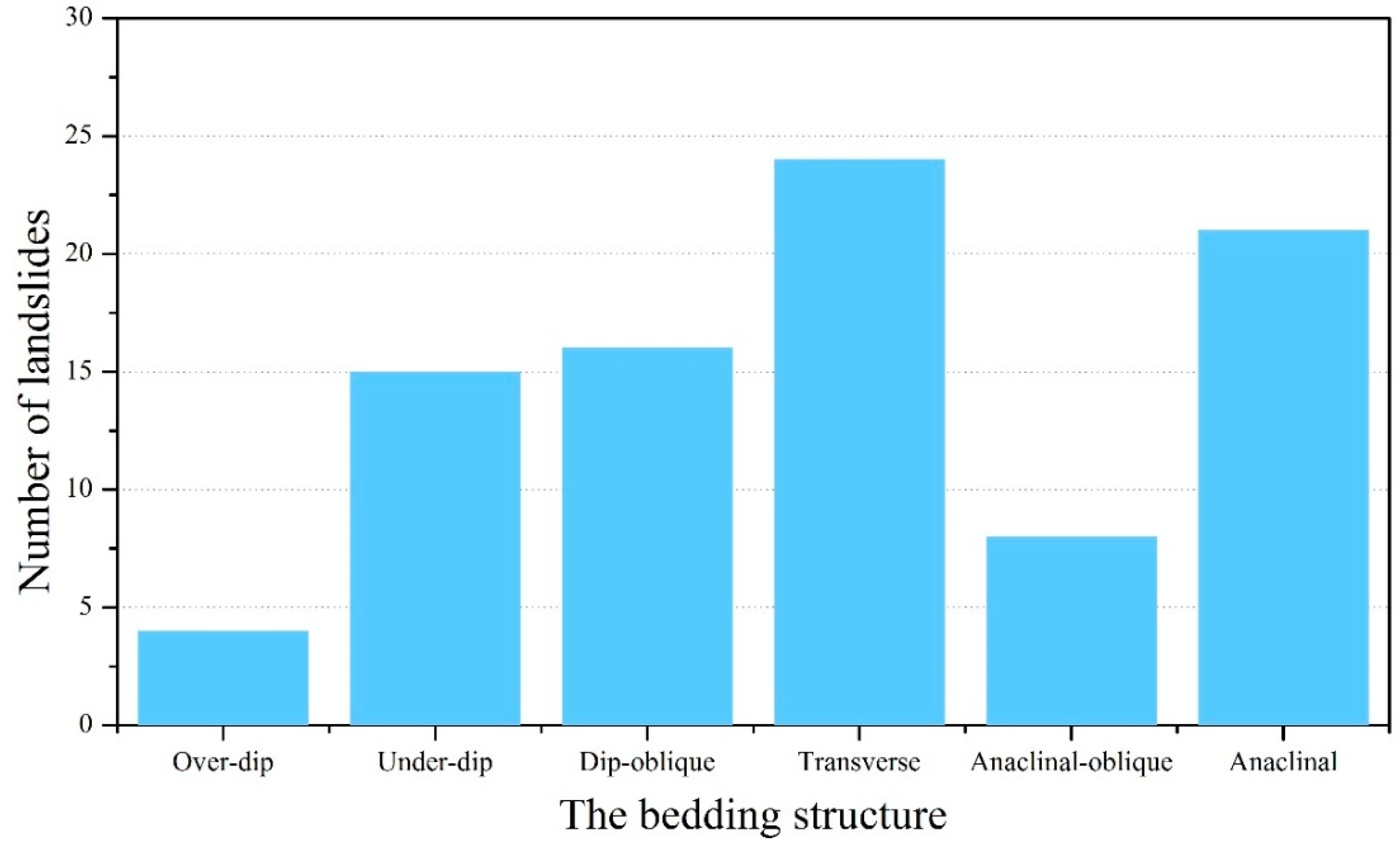
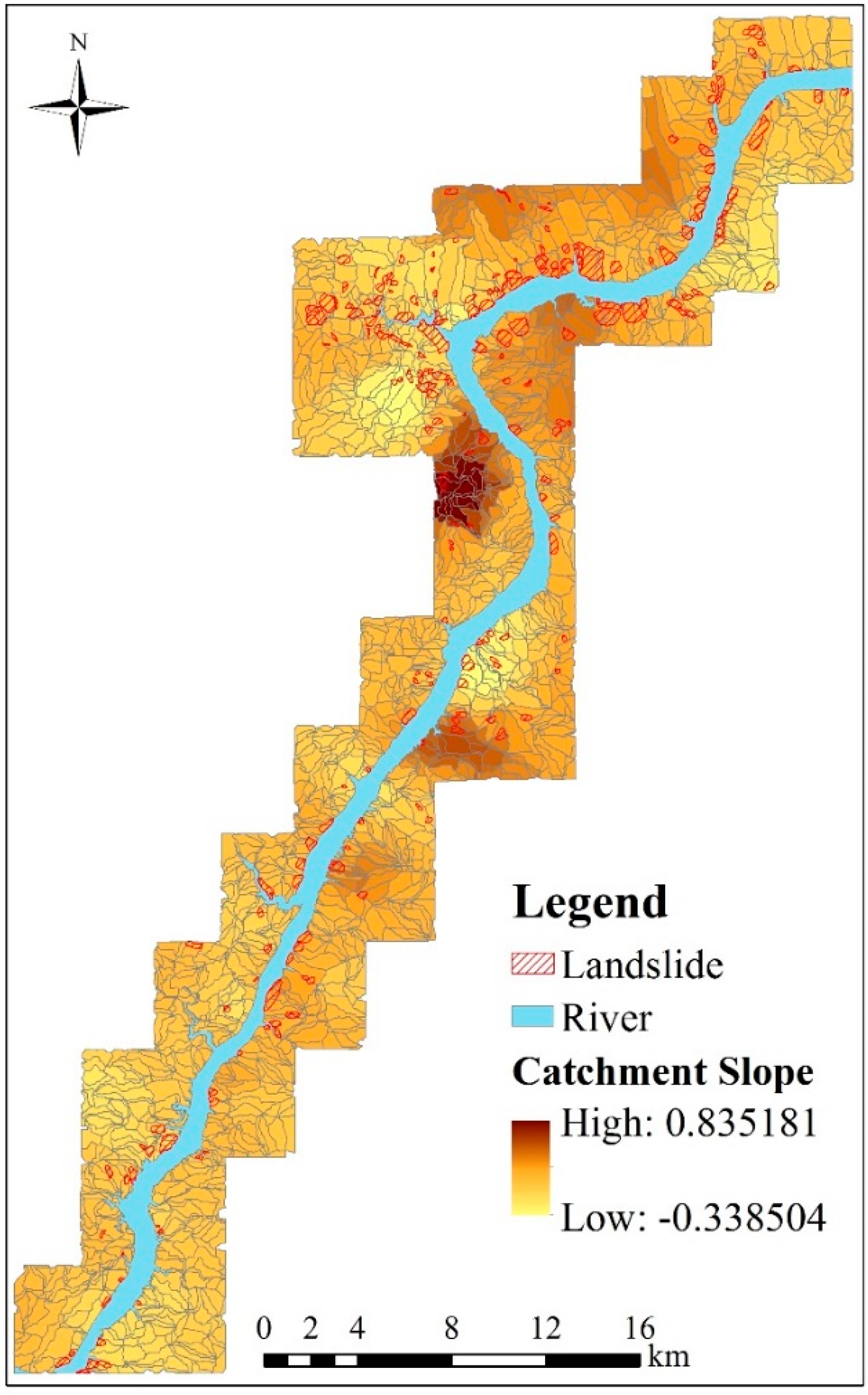
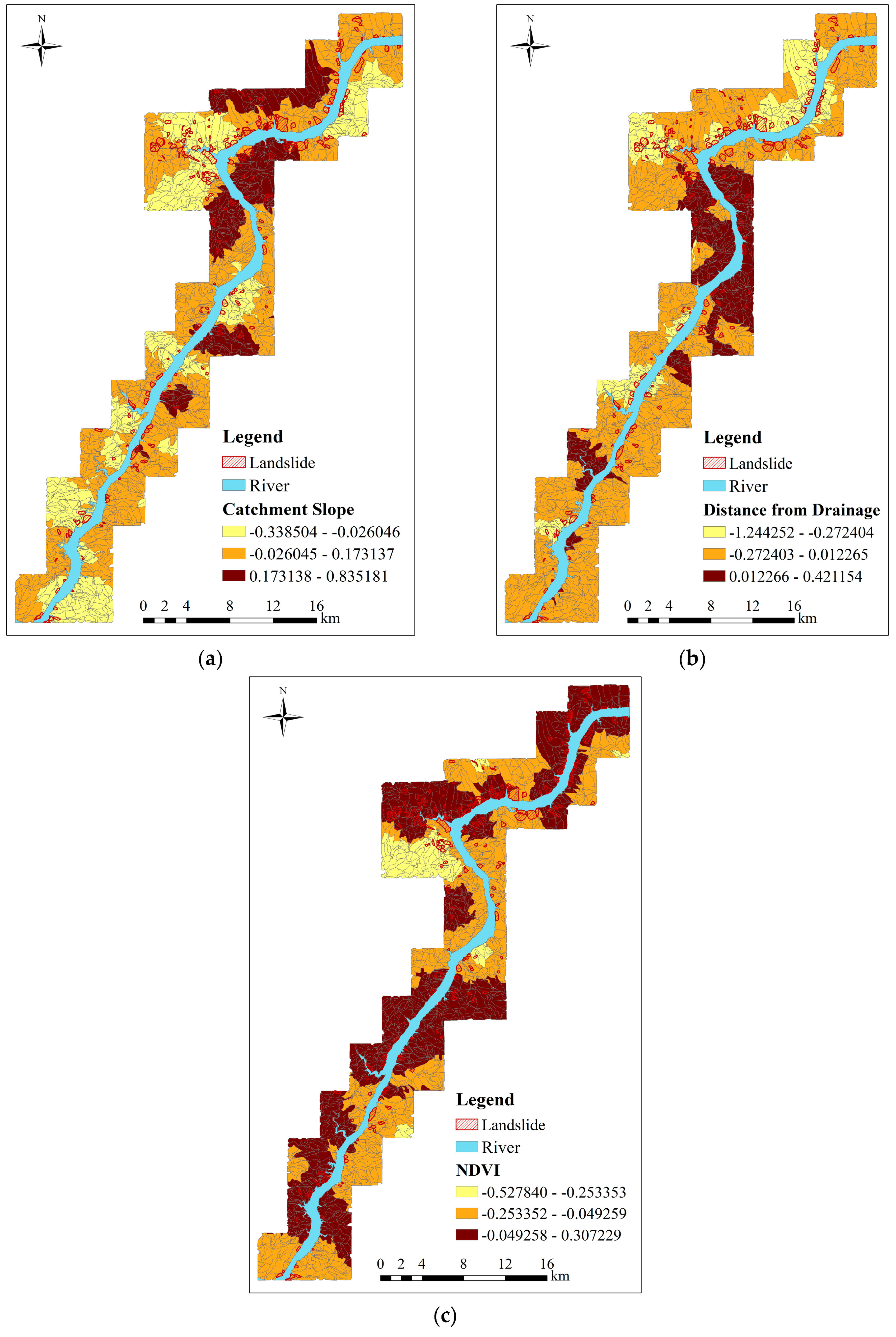
4.4. Environmental Factors of Landslides
- High-resolution aerial photographs;
- 1:50,000-Scale geological maps [55];
- ASTER G-DEM data with a spatial resolution of 30 m;
- Landsat-8 OLI+ sensor data, acquired on 24 February 2013, with the Path/Row number of 127/39 and its spatial resolution of 30 m for the extraction of land-use and calculation of Normalized Difference Vegetable Index (NDVI) and Normalized Difference Water Index (NDWI);
- Precipitation and seismic data from the China Meteorological Administration and the China Earthquake Administration for obtaining the precipitation and seismic factors.
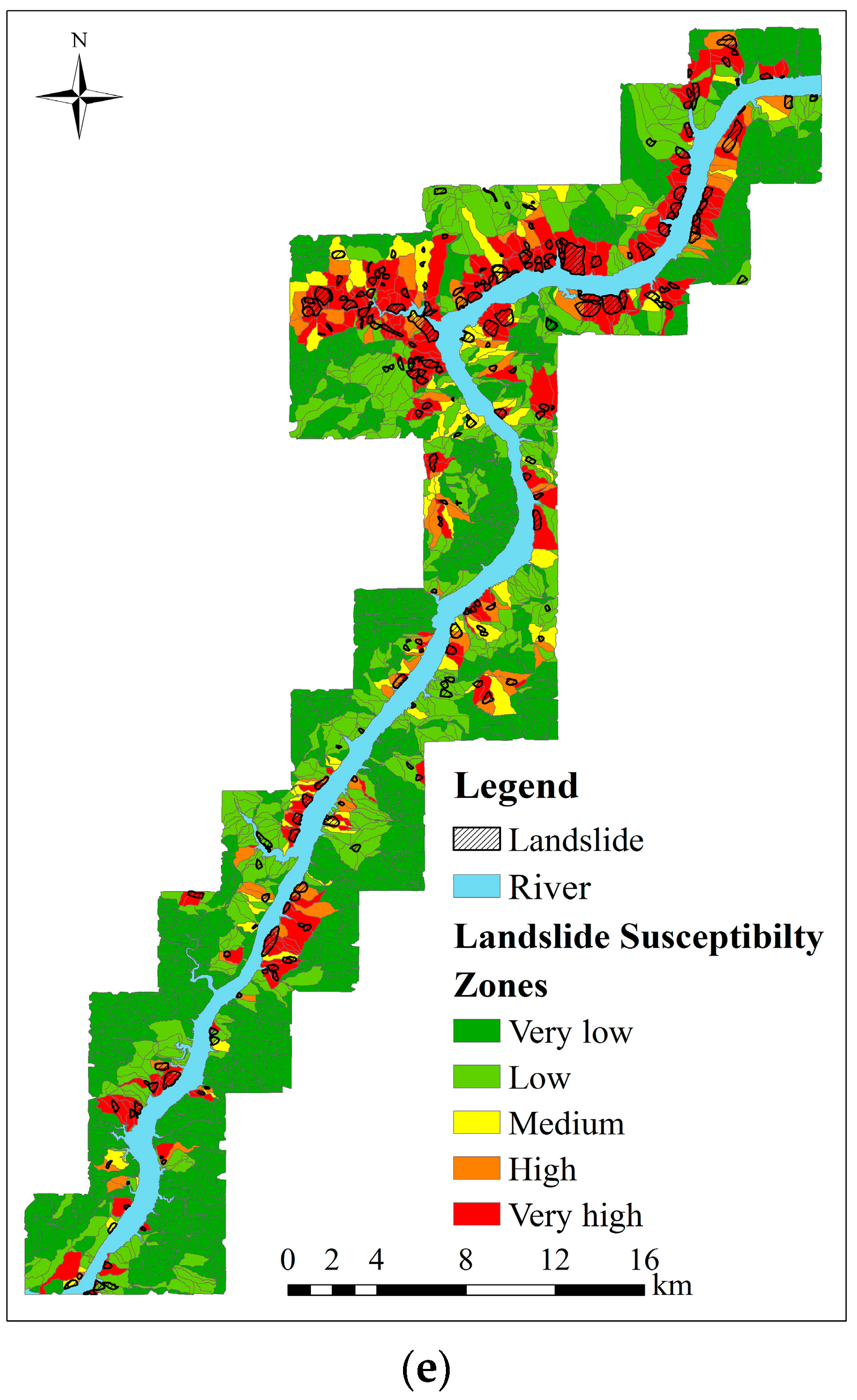
5. Results
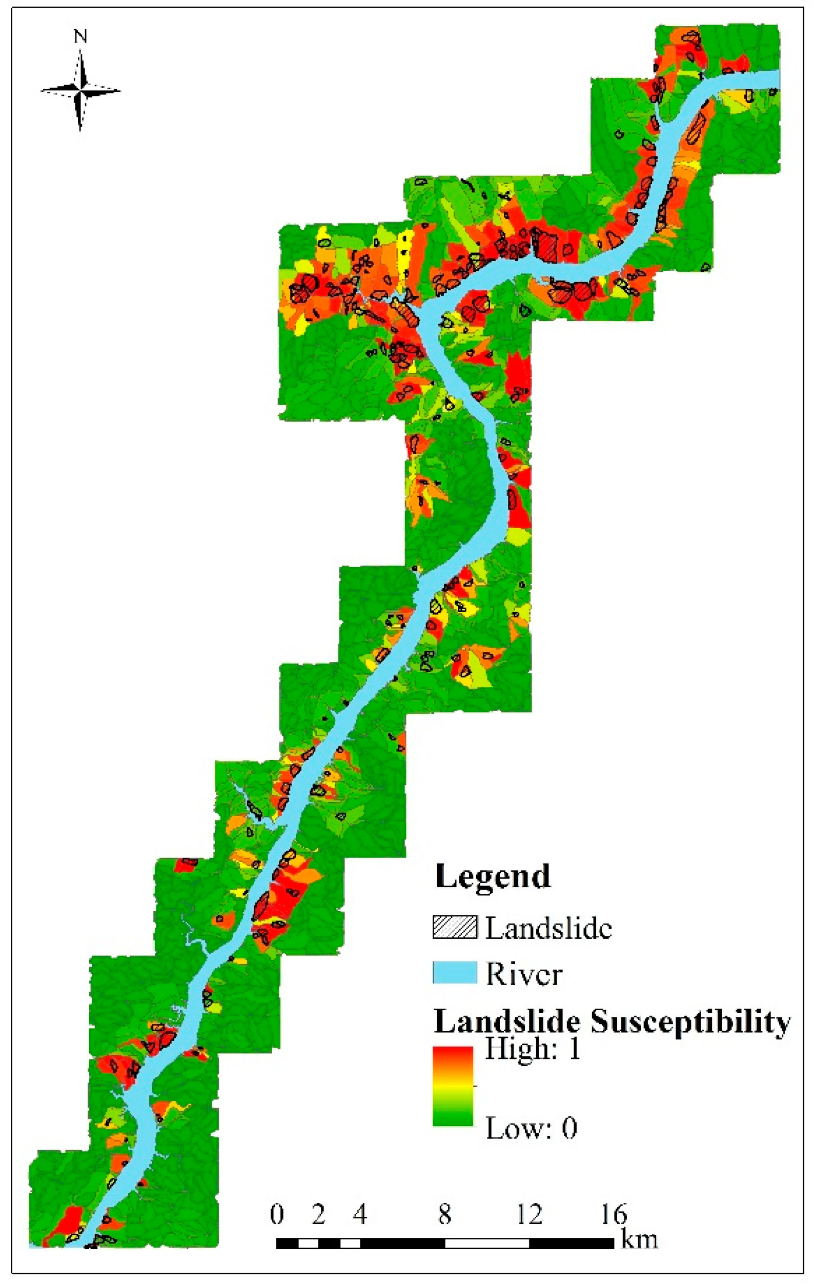
5.1. Experimental Results of The GWR-PSO-SVM Model
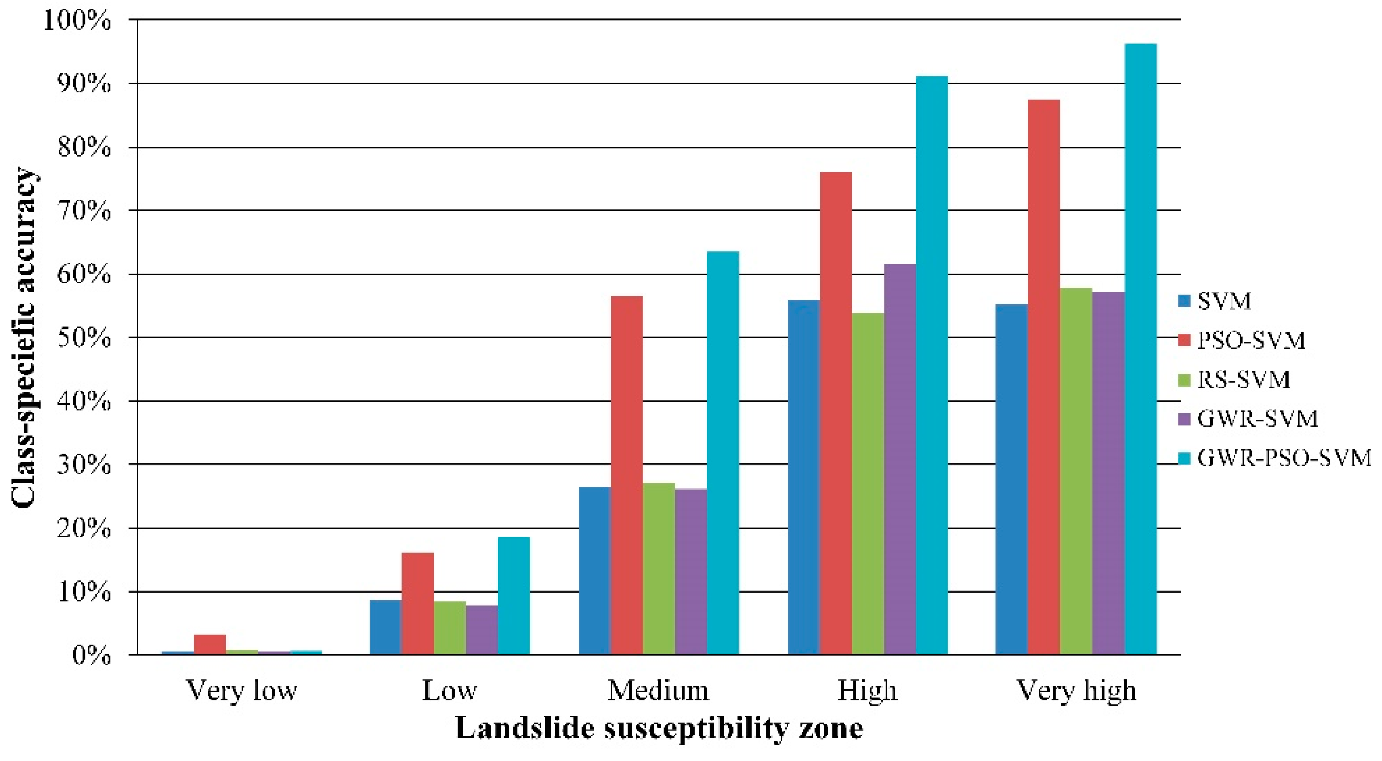
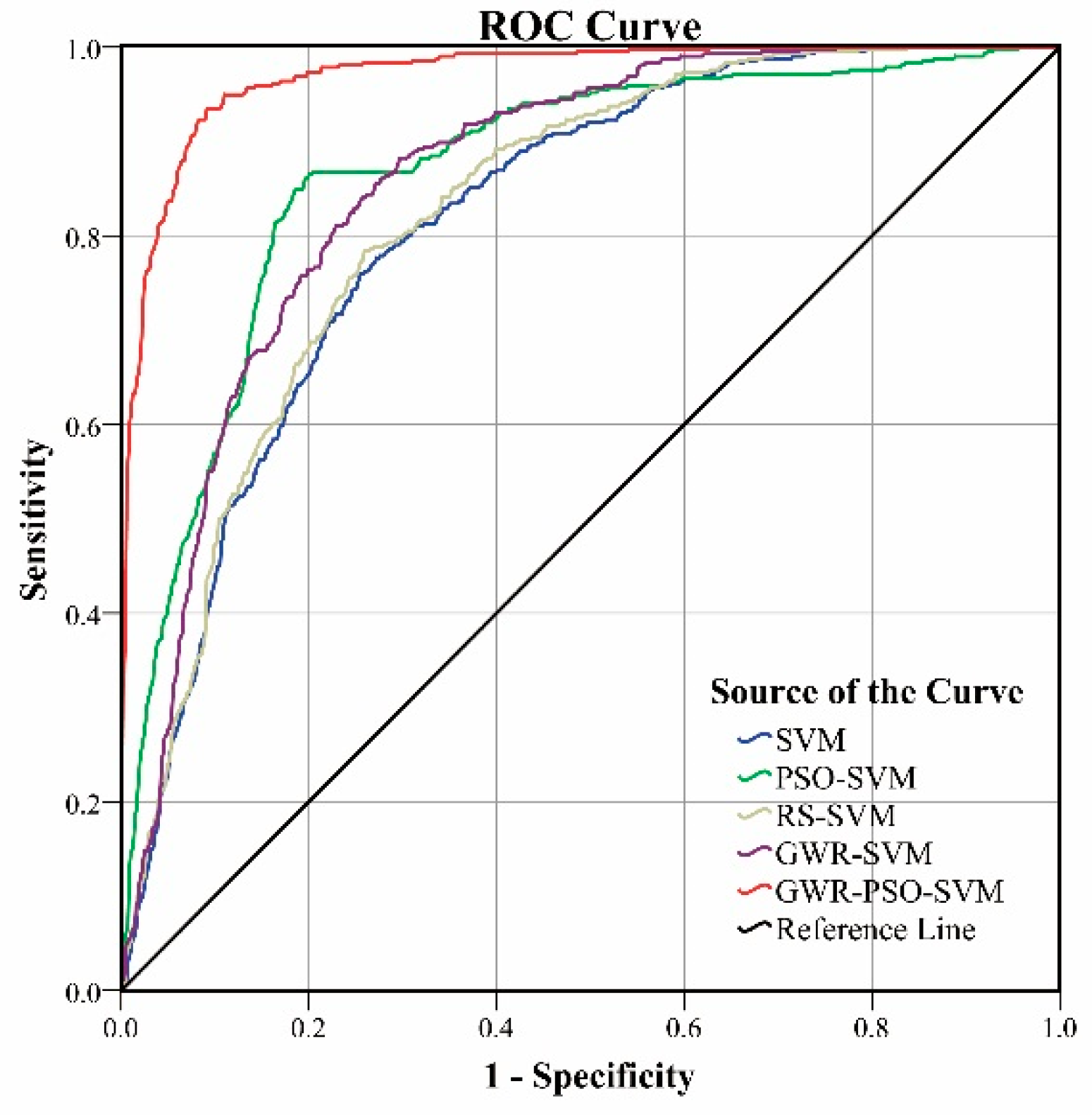
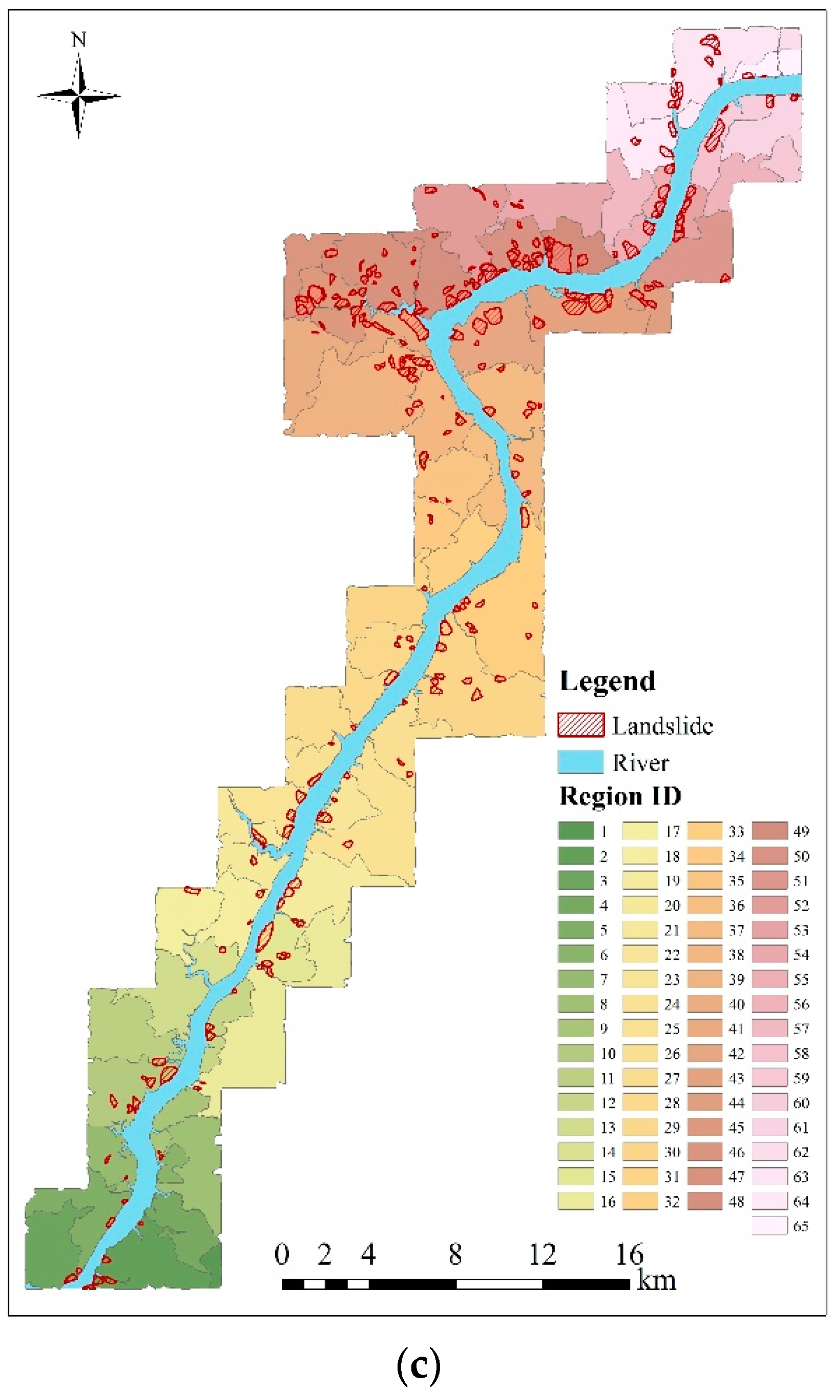
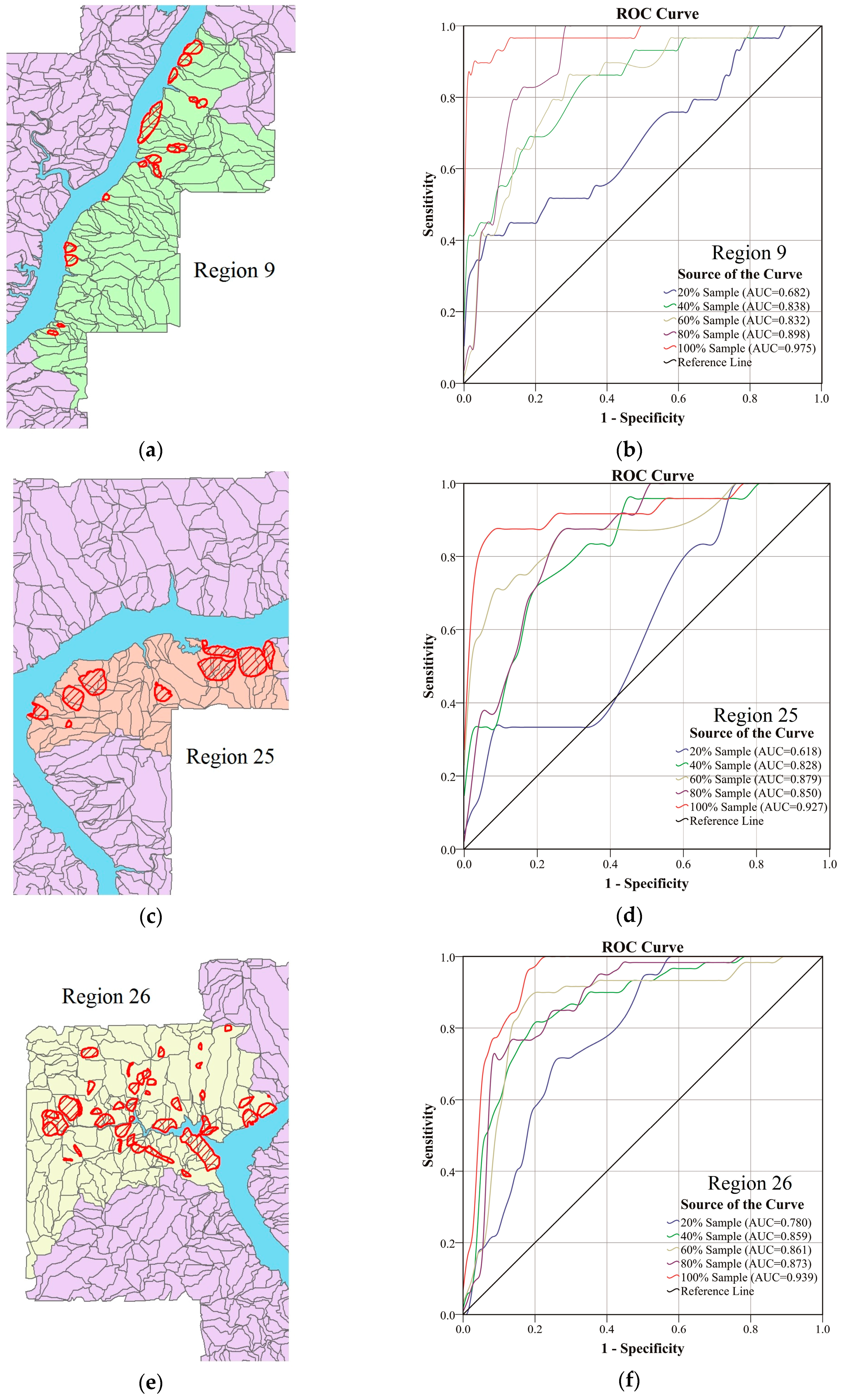
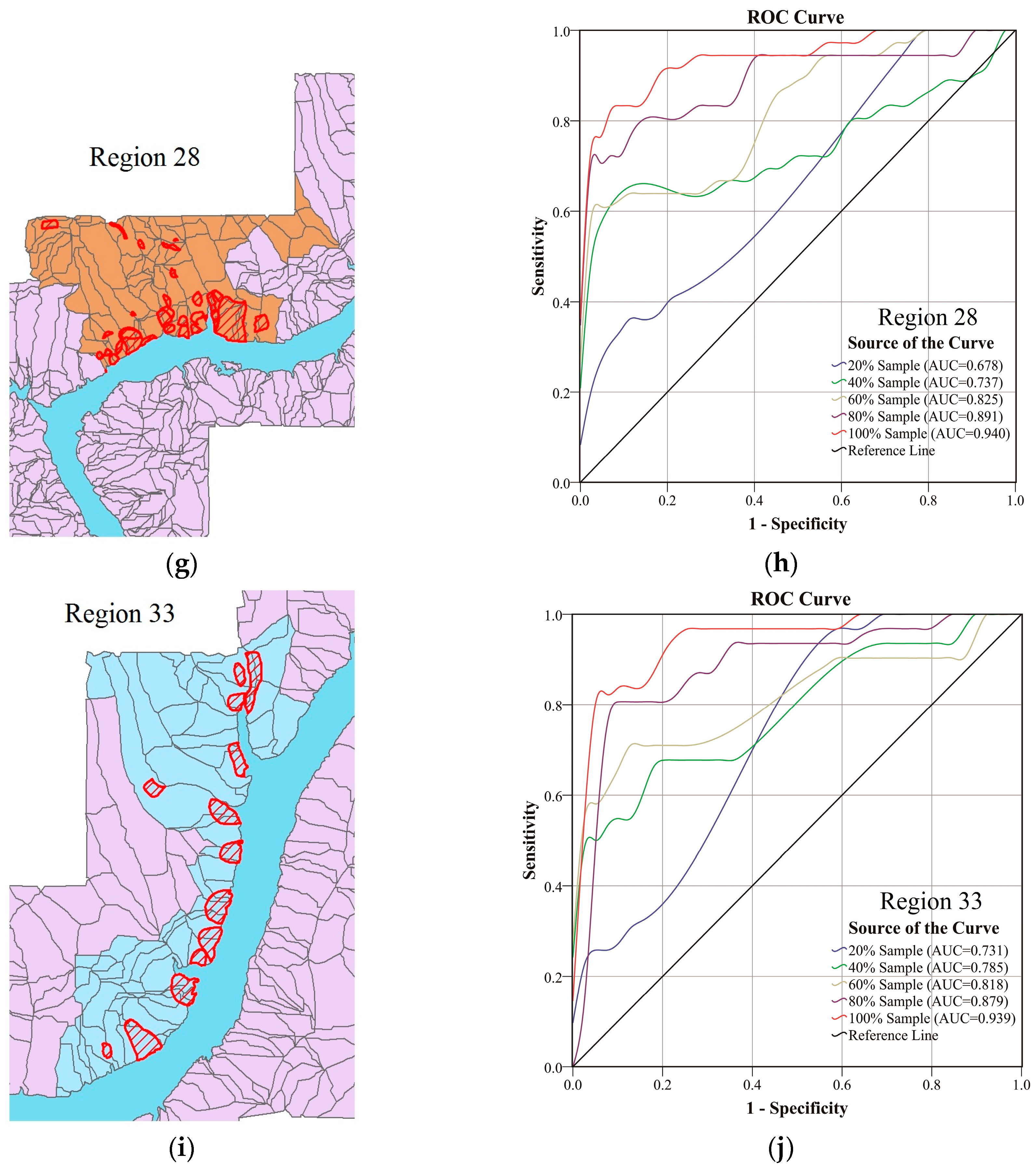
5.2. Methods to Assess Models Performance
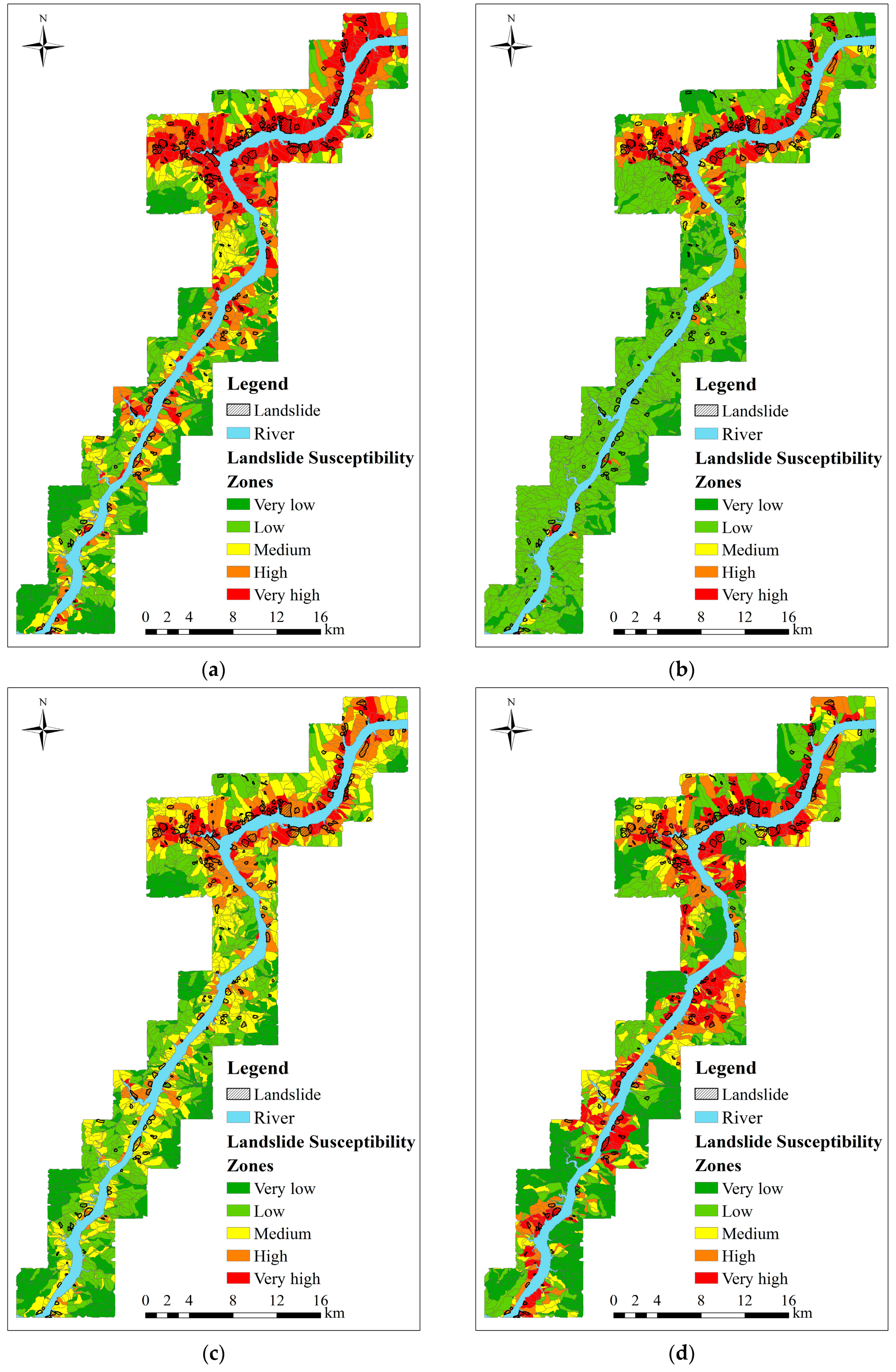
5.3. Comparison with Further Models
6. Discussion
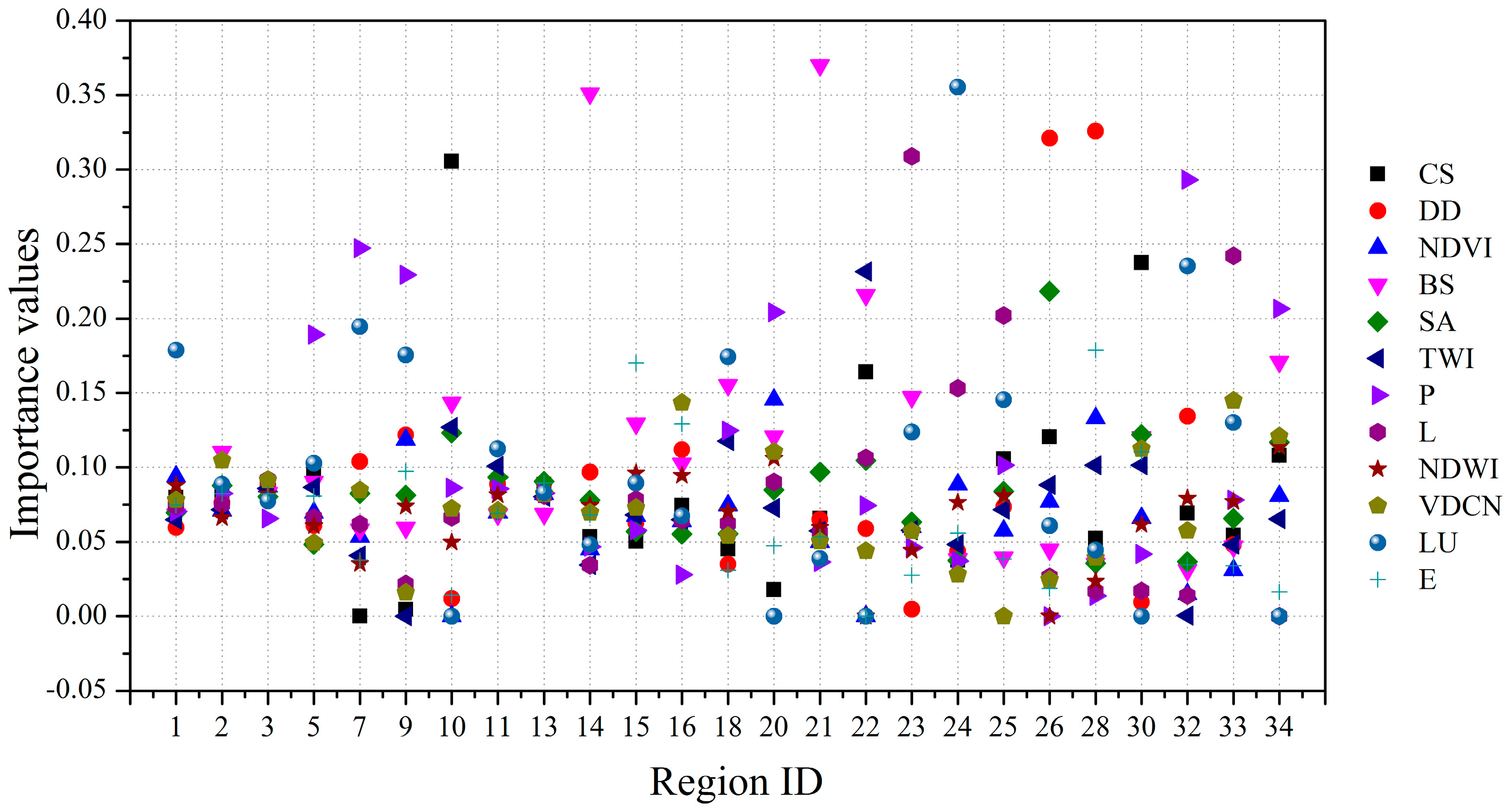
6.1. Impact of Environmental Factors
6.2. Influence of Regions Number
6.3. Model Sensitivity
7. Conclusions
Acknowledgments
Author Contributions
Conflicts of Interest
References
- Cruden, D.M.; Varnes, D.J. Landslides: Investigation and Mitigation; Chapter 3; Transportation Research Board Special Report: Washington, DC, USA, 1996. [Google Scholar]
- Liu, C.; Liu, Y.; Wen, M.; Li, T.; Lian, J.; Qin, S. Geo-hazard initiation and assessment in the three gorges reservoir. In Landslide Disaster Mitigation in Three Gorges Reservoir, China; Springer: Berlin, Germany, 2009; pp. 3–40. [Google Scholar]
- Brabb, E.E. The world landslide problem. In Episodes; US International Union of Geological Sciences (IUGS): Bangalore, India, 1991; Volume 14, pp. 52–61. [Google Scholar]
- Wan, S.; Chang, S.H. Combined particle swarm optimization and linear discriminant analysis for landslide image classification: Application to a case study in Taiwan. Environ. Earth Sci. 2014, 72, 1453–1464. [Google Scholar] [CrossRef]
- Regmi, N.R.; Giardino, J.R.; Vitek, J.D. Assessing susceptibility to landslides: Using models to understand observed changes in slopes. Geomorphology 2010, 122, 25–38. [Google Scholar] [CrossRef]
- Barredo, J.E.I.; Benavides, A.; Herv, A.S.J.; van Westen, C.J. Comparing heuristic landslide hazard assessment techniques using GIS in the Tirajana basin, Gran Canaria Island, Spain. Int. J. Appl. Earth Obs. Geoinf. 2000, 2, 9–23. [Google Scholar] [CrossRef]
- Dai, F.; Lee, C. Landslide characteristics and slope instability modeling using GIS, Lantau Island, Hong Kong. Geomorphology 2002, 42, 213–228. [Google Scholar] [CrossRef]
- Ohlmacher, G.C.; Davis, J.C. Using multiple logistic regression and GIS technology to predict landslide hazard in northeast Kansas, USA. Eng. Geol. 2003, 69, 331–343. [Google Scholar] [CrossRef]
- Ayalew, L.; Yamagishi, H. The application of gis-based logistic regression for landslide susceptibility mapping in the Kakuda-Yahiko Mountains, Central Japan. Geomorphology 2005, 65, 15–31. [Google Scholar] [CrossRef]
- Lee, S.; Ryu, J.H.; Min, K.; Won, J.S. Landslide susceptibility analysis using GIS and artificial neural network. Earth Surf. Process. Landforms 2003, 28, 1361–1376. [Google Scholar] [CrossRef]
- Gomez, H.; Kavzoglu, T. Assessment of shallow landslide susceptibility using artificial neural networks in Jabonosa River Basin, Venezuela. Eng. Geol. 2005, 78, 11–27. [Google Scholar] [CrossRef]
- Wang, H.; Sassa, K. Rainfall-induced landslide hazard assessment using artificial neural networks. Earth Surf. Process. Landforms 2006, 31, 235–247. [Google Scholar] [CrossRef]
- Melchiorre, C.; Matteucci, M.; Azzoni, A.; Zanchi, A. Artificial neural networks and cluster analysis in landslide susceptibility zonation. Geomorphology 2008, 94, 379–400. [Google Scholar] [CrossRef]
- Yao, X.; Tham, L.G.; Dai, F. Landslide susceptibility mapping based on support vector machine: A case study on natural slopes of Hong Kong, China. Geomorphology 2008, 101, 572–582. [Google Scholar] [CrossRef]
- Marjanović, M.; Kovačević, M.; Bajat, B.; Voženílek, V. Landslide susceptibility assessment using SVM machine learning algorithm. Eng. Geol. 2011, 123, 225–234. [Google Scholar] [CrossRef]
- Ballabio, C.; Sterlacchini, S. Support vector machines for landslide susceptibility mapping: The Staffora River Basin case study, Italy. Math. Geosci. 2012, 44, 47–70. [Google Scholar] [CrossRef]
- Xu, C.; Dai, F.; Xu, X.; Lee, Y.H. GIS-based support vector machine modeling of earthquake-triggered landslide susceptibility in the Jianjiang River watershed, China. Geomorphology 2012, 145, 70–80. [Google Scholar] [CrossRef]
- Erener, A.; Düzgün, H.S.B. Improvement of statistical landslide susceptibility mapping by using spatial and global regression methods in the case of More and Romsdal (Norway). Landslides 2010, 7, 55–68. [Google Scholar] [CrossRef]
- Sabokbar, H.F.; Roodposhti, M.S.; Tazik, E. Landslide susceptibility mapping using geographically-weighted principal component analysis. Geomorphology 2014, 226, 15–24. [Google Scholar] [CrossRef]
- San, B.T. An evaluation of svm using polygon-based random sampling in landslide susceptibility mapping: The Candir Catchment area (Western Antalya, Turkey). Int. J. Appl. Earth Obs. 2014, 26, 399–412. [Google Scholar] [CrossRef]
- Yao, X.; Zhang, Y.; Zhou, N.; Guo, C.; Yu, K.; Li, L.J. Application of two-class SVM applied in landslide susceptibility mapping. In Project Planning and Project Success: The 25% Solution; Taylor & Francis Group: England, UK, 2014; p. 203. [Google Scholar]
- Huang, C.-L.; Dun, J.-F. A distributed PSO–SVM hybrid system with feature selection and parameter optimization. Appl. Soft Comput. 2008, 8, 1381–1391. [Google Scholar] [CrossRef]
- Zhao, H.; Yin, S. Geomechanical parameters identification by particle swarm optimization and support vector machine. Appl. Math. Model. 2009, 33, 3997–4012. [Google Scholar] [CrossRef]
- Ren, F.; Wu, X.; Zhang, K.; Niu, R. Application of wavelet analysis and a particle swarm-optimized support vector machine to predict the displacement of the shuping landslide in the Three Gorges, China. Environ. Earth Sci. 2015, 73, 4791–4804. [Google Scholar] [CrossRef]
- Kennedy, J.; Eberhart, R. Particle swarm optimization. In Proceedings of the IEEE International of First Conference on Neural Networks, Perth, Australia, 27 November 1995–1 December 1995; pp. 1942–1948.
- Holland, J.H. Genetic algorithms and the optimal allocation of trials. SIAM J. Comput. 1973, 2, 88–105. [Google Scholar] [CrossRef]
- Hassan, R.; Cohanim, B.; De Weck, O.; Venter, G. A comparison of particle swarm optimization and the genetic algorithm. In Proceedings of the 46th AIAA Multidisciplinary Design Optimization Specialist Conference, Austin, Texas, 18–21 April 2005; pp. 18–21.
- Brunsdon, C.; Fotheringham, A.S.; Charlton, M.E. Geographically weighted regression: A method for exploring spatial nonstationarity. Geogr. Anal. 1996, 28, 281–298. [Google Scholar] [CrossRef]
- Fotheringham, A.S.; Charlton, M.; Brunsdon, C. The geography of parameter space: An investigation of spatial non-stationarity. Int. J. Geogr. Inf. Syst. 1996, 10, 605–627. [Google Scholar] [CrossRef]
- Schabenberger, O.; Gotway, C.A. Statistical Methods for Spatial Data Analysis; CRC Press: Boca Raton, FL, USA, 2004. [Google Scholar]
- Fischer, M.M.; Getis, A. Handbook of applied spatial analysis: Software tools, methods and applications. Springer Science & Business Media: Berlin, Germany, 2009. [Google Scholar]
- Nakaya, T. Local spatial interaction modelling based on the geographically weighted regression approach. In Modelling Geographical Systems; Springer: Dordrecht, The Netherlands, 2002; pp. 45–69. [Google Scholar]
- Fotheringham, A.S.; Brunsdon, C.; Charlton, M. Geographically Weighted Regression: The Analysis of Spatially Varying Relationships; John Wiley & Sons: New York, NY, USA, 2003. [Google Scholar]
- Feuillet, T.; Coquin, J.; Mercier, D.; Cossart, E.; Decaulne, A.; Jónsson, H.P.; Sæmundsson, B. Focusing on the spatial non-stationarity of landslide predisposing factors in Northern Iceland: Do paraglacial factors vary over space? Prog. Phys. Geogr. 2014, 38, 354–377. [Google Scholar] [CrossRef]
- Brunsdon, C.; Fotheringham, S.; Charlton, M. Spatial nonstationarity and autoregressive models. Environ. Plann. A 1998, 30, 957–973. [Google Scholar] [CrossRef]
- Wheeler, D.C. Geographically weighted regression. In Handbook of Regional Science; Springer: Berlin, Germany, 2014; pp. 1435–1459. [Google Scholar]
- Fotheringham, A.S.; Charlton, M.; Brunsdon, C. Measuring spatial variations in relationships with geographically weighted regression. In Recent Developments in Spatial Analysis; Springer: Berlin, Germany, 1997; pp. 60–82. [Google Scholar]
- Chalkias, C.; Kalogirou, S.; Ferentinou, M. Landslide susceptibility, Peloponnese peninsula in south Greece. J. Maps 2014, 10, 211–222. [Google Scholar] [CrossRef]
- Fotheringham, A.S.; Charlton, M.; Brunsdon, C. Geographically weighted regression: A natural evolution of the expansion method for spatial data analysis. Environ. Plan. A 1998, 30, 1905–1927. [Google Scholar] [CrossRef]
- Celik, M.; Kazar, B.M.; Shekhar, S.; Boley, D. Parameter Estimation for the Spatial Autoregression Model: A Rigorous Approach. Available online: http://www-users.cs.umn.edu/~boley/publications/papers/NASA06.pdf (accessed on 23 February 2016).
- Cleveland, W.S. Robust locally weighted regression and smoothing scatterplots. J. Am. Stat. Assoc. 1979, 368, 829–836. [Google Scholar] [CrossRef]
- Hirotugu, A. A new look at the statistical model identification. Autom. Control Comput. Sci. 1974, 6, 716–723. [Google Scholar]
- Vapnik, V.N. The Nature of Statistical Learning Theory; Springer New York: New York, NY, USA, 1995. [Google Scholar]
- Barakat, N.; Bradley, A.P. Rule extraction from support vector machines: A review. Neurocomputing 2010, 74, 178–190. [Google Scholar] [CrossRef]
- Mountrakis, G.; Im, J.; Ogole, C. Support vector machines in remote sensing: A review. ISPRS J. Photogramm. Remote Sens. 2011, 66, 247–259. [Google Scholar] [CrossRef]
- Peng, L.; Niu, R.; Huang, B.; Wu, X.; Zhao, Y.; Ye, R. Landslide susceptibility mapping based on rough set theory and support vector machines: A case of the Three Gorges Area, China. Geomorphology 2014, 204, 287–301. [Google Scholar] [CrossRef]
- Suykens, J.A.; Vandewalle, J. Least squares support vector machine classifiers. Neural Process. Lett. 1999, 9, 293–300. [Google Scholar] [CrossRef]
- Kennedy, J. Particle swarm optimization. In Encyclopedia of Machine Learning; Springer: Berlin, Germany, 2011; pp. 760–766. [Google Scholar]
- Xiao, C.; Hao, K.; Ding, Y. The bi-directional prediction of carbon fiber production using a combination of improved particle swarm optimization and support vector machine. Materials 2014, 8, 117–136. [Google Scholar] [CrossRef]
- Zhang, L.; Bi, H.; Cheng, P.; Davis, C.J. Modeling spatial variation in tree diameter–height relationships. For. Ecol. Manag. 2004, 189, 317–329. [Google Scholar] [CrossRef]
- Miller, H.J. Tobler’s first law and spatial analysis. Ann. Assoc. Am. Geogr. 2004, 94, 284–289. [Google Scholar] [CrossRef]
- Jenks, G.F. The data model concept in statistical mapping. Int. Yearb. Cartogr. 1967, 7, 186–190. [Google Scholar]
- Li, J.; Xie, S.; Kuang, M. Geomorphic evolution of the yangtze gorges and the time of their formation. Geomorphology 2001, 41, 125–135. [Google Scholar] [CrossRef]
- Zhou, Q.; Lv, Z.; Ma, Z.; Zhang, Y.; Wang, H. Barrier belt division based on rs and gis in the three gorges reservoir area—A case of Wanzhou district. Procedia. Environ. Sci. 2011, 10, 1257–1263. [Google Scholar] [CrossRef]
- Hubei Province Geological Survey. Geological Map of Zigui and Badong County (1:50,000); Hubei Province Geological Survey Press: Wuhan, China, 1997. [Google Scholar]
- Headquarters of Prevention and Control of Geo-Hazards in Area of Three Gorges Reservoir; 1:10,000 Geological Hazard Mapping Database: Yichang, China, 2011.
- Guzzetti, F.; Carrara, A.; Cardinali, M.; Reichenbach, P. Landslide hazard evaluation: A review of current techniques and their application in a multi-scale study, central Italy. Geomorphology 1999, 31, 181–216. [Google Scholar] [CrossRef]
- Liu, J.G.; Mason, P.J.; Clerici, N.; Chen, S.; Davis, A.; Miao, F.; Deng, H.; Liang, L. Landslide hazard assessment in the three gorges area of the Yangtze River using ASTER imagery: Zigui–Badong. Geomorphology 2004, 61, 171–187. [Google Scholar] [CrossRef]
- Meentemeyer, R.K.; Moody, A. Automated mapping of conformity between topographic and geological surfaces. Comput. Geosci. 2000, 26, 815–829. [Google Scholar] [CrossRef]
- Kunlong, Y.; Wenxing, J.; Yang, W.; Chunmei, Z.; Changqian, M.; Liling, L.; Lingling, Y.; Yiping, W. The Research of Three Gorges Reservoir in Wanzhou Area of Nearly Horizontal Strata Landslide Formation Mechanism and Control Engineering; China University of Geosciences Press: Wuhan, China, 2007; pp. 39–65. [Google Scholar]
- Chen, T.; Niu, R.; Du, B.; Wang, Y. Landslide spatial susceptibility mapping by using GIS and Remote Sensing techniques: A case study in Zigui county, the Three Georges Reservoir, China. Environ. Earth Sci. 2015, 73, 5571–5583. [Google Scholar] [CrossRef]
- Zweig, M.H.; Campbell, G. Receiver-operating characteristic (ROC) plots: A fundamental evaluation tool in clinical medicine. Clin. Chem. 1993, 39, 561–577. [Google Scholar] [PubMed]
- Pawlak, Z. Rough sets. Int. J. Comput. Inf. Sci. 1982, 11, 341–356. [Google Scholar] [CrossRef]
- Liu, J.; Zeng, Z.; Liu, H.; Wang, H. A rough set approach to analyze factors affecting landslide incidence. Comput. Geosci. 2011, 37, 1311–1317. [Google Scholar] [CrossRef]
- Komorowski, J.; Pawlak, Z.; Polkowski, L.; Skowron, A. Rough Sets: A Tutorial. Available online: http://eecs.ceas.uc.edu/~mazlack/dbm.w2011/Komorowski.RoughSets.tutor.pdf (accessed on 23 February 2016).
- Pawlak, Z. Rough Sets: Theoretical Aspects of Reasoning about Data; Springer Science & Business Media: Berlin, Germany, 2012. [Google Scholar]
- Pawlak, Z.; Sowinski, R. Rough set approach to multi-attribute decision analysis. Eur. J. Oper. Res. 1994, 72, 443–459. [Google Scholar] [CrossRef]
- Kryszkiewicz, M. Rough set approach to incomplete information systems. Inf. Sci. 1998, 112, 39–49. [Google Scholar] [CrossRef]
- Swiniarski, R.W.; Skowron, A. Rough set methods in feature selection and recognition. Pattern. Recognit. Lett. 2003, 24, 833–849. [Google Scholar] [CrossRef]
- Davvaz, B. Roughness based on fuzzy ideals. Inf. Sci. 2006, 176, 2417–2437. [Google Scholar] [CrossRef]
- Gorsevski, P.V.; Jankowski, P. Discerning landslide susceptibility using rough sets. Comput. Environ. Urban Syst. 2008, 32, 53–65. [Google Scholar] [CrossRef]
- Thangavel, K.; Pethalakshmi, A. Dimensionality reduction based on rough set theory: A review. Appl. Soft Comput. 2009, 9, 1–12. [Google Scholar] [CrossRef]
- Pan, X.; Zhang, S.; Zhang, H.; Na, X.; Li, X. A variable precision rough set approach to the remote sensing land use/cover classification. Comput. Geosci. 2010, 36, 1466–1473. [Google Scholar] [CrossRef]
- Leung, Y.; Fung, T.; Mi, J.S.; Wu, W.Z. A rough set approach to the discovery of classification rules in spatial data. Int. J. Geogr. Inf. Sci. 2007, 21, 1033–1058. [Google Scholar] [CrossRef]


| Input: Training and Verification Samples. |
| Output: The Result of the PSO-SVM Model. |
|
|
|
|
|
|
|
|
|
|
|
|
| Input: Ancillary Data of the Study Area. |
|---|
| Output: The Landslide Susceptibility Map. |
Step 1: Extract environmental factors
|
Step 2: Environmental factors screening
|
Step 3: Study area segmentation
|
Step 4: The PSO-SVM prediction
|
| Type | Definition |
|---|---|
| Over-dip slope | |
| Under-dip slope | |
| Dip-oblique slope | |
| Transverse slope | |
| Anaclinal-oblique slope | |
| Anaclinal slope |
| Environmental Factors | Value | |
|---|---|---|
| Geomorphology | Elevation (m) | 124.2727–922.3077 |
| Slope angle (°) | 3.2045–36.2898 | |
| Slope aspect (°) | 28.4827–321.5051 | |
| Terrain surface convexity (°/100m) | 0.5979–0.2449 | |
| Plane curvature (°/100m) | −0.4023–0.4832 | |
| Profile curvature (°/100m) | −1.2441–1.2856 | |
| Slope form | (1) V/V; (2) GE/V; (3) X/V; (4) V/GR; (5) GE/GR; (6) X/GR; (7) V/X; (8) GE/X; (9) X/X | |
| Slope height (m) | 374.6390–3.6325 | |
| Mid-slope position | 0.1272–0.9491 | |
| Terrain surface texture | 0.8495–0.3018 | |
| Terrain roughness index | 1.1589–16.4521 | |
| Terrain convergence index | −27.6027–19.7669 | |
| Terrain curvature (°/100m) | −1.5762–1.4682 | |
| Terrain position index | −14.6285–9.5591 | |
| Geology | Lithology | (1) mudstone, shale and Quaternary deposits; (2) sandstones and thinly bedded limestones; (3) limestones and massive sandstones |
| Bedding structure | (1) over-dip slope; (2) under-dip slope; (3) dip-oblique slope; (4) transverse slope; (5) anaclinal-oblique slope; (6) anaclinal slope | |
| Hydrology | Catchment area (m2) | 1156.0378–105,783.4666 |
| Catchment slope (°) | 0.0485–0.5675 | |
| Flow path length (m) | 50.1196–2352.5587 | |
| Valley depth (m) | 3.4642–258.2873 | |
| Stream power index | −617,299.4571–281,486.9383 | |
| Distance from drainage (m) | 18.4328–5637.6471 | |
| Topographic wetness index | 8.2193–14.7816 | |
| Vertical distance to channel network (m) | −184.3475–461.4196 | |
| Land cover | Land-use | (1) water; (2) residential; (3) forest; (4) agriculture; (5) grassland |
| NDVI | −0.4856–0.8337 | |
| NDWI | 0.0206–0.69411 | |
| Meteorology | Precipitation (mm) | 1134.0551–1192.7400 |
| Geophysics | Magnitude (Ms) | 1.2617–2.1209 |
| Environmental Factor | ELE | SLAN | SLAS | SLHE | SLFO | TST | TRI | TPI | TCI | MSLP | PLCU | PRCU | TCU | TSC |
|---|---|---|---|---|---|---|---|---|---|---|---|---|---|---|
| ELE | 1 | |||||||||||||
| SLAN | 0.198 | 1 | ||||||||||||
| SLAS | 0.022 | −0.099 | 1 | |||||||||||
| SLHE | 0.321 | 0.581 | 0.03 | 1 | ||||||||||
| SLFO | −0.013 | 0.093 | 0.16 | 0.206 | 1 | |||||||||
| TST | −0.255 | −0.739 | 0.045 | −0.562 | −0.022 | 1 | ||||||||
| TRI | 0.188 | 0.995 | −0.105 | 0.579 | 0.091 | −0.735 | 1 | |||||||
| TPI | 0.125 | 0.138 | 0.122 | 0.338 | 0.761 | −0.062 | 0.133 | 1 | ||||||
| TCI | 0.117 | 0.054 | 0.221 | 0.241 | 0.787 | −0.013 | 0.047 | 0.810 | 1 | |||||
| MSLP | 0.08 | 0.007 | 0.015 | 0.176 | −0.163 | −0.143 | 0.025 | −0.15 | −0.16 | 1 | ||||
| PLCU | −0.103 | 0.112 | 0.187 | 0.162 | 0.735 | −0.052 | 0.114 | 0.601 | 0.641 | −0.093 | 1 | |||
| PRCU | −0.172 | −0.103 | −0.08 | −0.224 | −0.564 | 0.017 | −0.095 | −0.809 | −0.661 | 0.14 | −0.3 | 1 | ||
| TCU | 0.071 | 0.131 | 0.155 | 0.243 | 0.782 | −0.04 | 0.127 | 0.889 | 0.804 | −0.15 | 0.728 | −0.872 | 1 | |
| TSC | 0.083 | 0.155 | −0.015 | 0.356 | 0.169 | 0.172 | 0.142 | 0.204 | 0.165 | 0.021 | 0.034 | −0.2 | 0.161 | 1 |
| Environmental Factor | DISD | CMA | FPL | TWI | VADE | CMSL | SPI | VDCN |
|---|---|---|---|---|---|---|---|---|
| DISD | 1 | |||||||
| CMA | 0.011 | 1 | ||||||
| FPL | −0.109 | 0.551 | 1 | |||||
| TWI | −0.026 | 0.607 | 0.545 | 1 | ||||
| VADE | −0.112 | 0.678 | 0.675 | 0.65 | 1 | |||
| CMSL | −0.007 | 0.327 | 0.41 | 0.411 | 0.638 | 1 | ||
| SPI | −0.055 | −0.013 | 0.004 | −0.112 | −0.052 | −0.004 | 1 | |
| VDCN | −0.368 | 0.259 | 0.424 | 0.222 | 0.475 | 0.292 | 0.045 | 1 |
| Region ID | Number of Slope-Units | Number of Landslide Slope-Units | Region ID | Number of Slope-Units | Number of Landslide Slope-Units |
|---|---|---|---|---|---|
| 1 | 59 | 9 | 18 | 75 | 18 |
| 2 | 51 | 5 | 19 | 40 | 0 |
| 3 | 8 | 2 | 20 | 63 | 14 |
| 4 | 59 | 0 | 21 | 52 | 12 |
| 5 | 52 | 5 | 22 | 54 | 12 |
| 6 | 17 | 0 | 23 | 52 | 13 |
| 7 | 61 | 19 | 24 | 57 | 15 |
| 8 | 61 | 0 | 25 | 71 | 24 |
| 9 | 138 | 29 | 26 | 134 | 60 |
| 10 | 57 | 9 | 27 | 10 | 0 |
| 11 | 38 | 12 | 28 | 80 | 36 |
| 12 | 80 | 0 | 29 | 9 | 0 |
| 13 | 21 | 2 | 30 | 76 | 12 |
| 14 | 90 | 23 | 31 | 7 | 0 |
| 15 | 64 | 8 | 32 | 47 | 22 |
| 16 | 77 | 14 | 33 | 70 | 31 |
| 17 | 42 | 0 | 34 | 37 | 10 |
| GWR-PSO-SVM Model | Region ID | C | γ | Region ID | C | γ |
| 1 | 6.1826 | 0.13879 | 20 | 5.9453 | 0.29134 | |
| 2 | 1.2965 | 0.32455 | 21 | 5.3659 | 0.38439 | |
| 3 | 2.4682 | 0.31596 | 22 | 3.3548 | 0.17105 | |
| 5 | 1.4832 | 0.36957 | 23 | 5.8234 | 0.36851 | |
| 7 | 8.6235 | 0.51243 | 24 | 2.1629 | 0.47592 | |
| 9 | 4.1356 | 0.67572 | 25 | 3.2592 | 0.45665 | |
| 10 | 2.3659 | 0.49986 | 26 | 6.5359 | 0.67853 | |
| 11 | 2.6971 | 0.33645 | 28 | 6.2157 | 0.47935 | |
| 13 | 4.3651 | 0.42631 | 30 | 7.2853 | 0.63428 | |
| 14 | 5.8652 | 0.42375 | 32 | 6.4075 | 3.35874 | |
| 15 | 1.4964 | 0.56916 | 33 | 5.3364 | 0.47516 | |
| 16 | 4.7569 | 0.32793 | 34 | 4.8435 | 0.67203 | |
| 18 | 1.4259 | 0.47157 | - | |||
| Model | Region ID | Training Sample | Verification Sample | Region ID | Training Sample | Verification Sample |
|---|---|---|---|---|---|---|
| GWR-PSO-SVM and GWR-SVM | 1 | 18 | 59 | 20 | 28 | 63 |
| 2 | 10 | 51 | 21 | 24 | 52 | |
| 3 | 4 | 8 | 22 | 24 | 54 | |
| 5 | 10 | 52 | 23 | 26 | 52 | |
| 7 | 38 | 61 | 24 | 30 | 57 | |
| 9 | 58 | 138 | 25 | 48 | 71 | |
| 10 | 18 | 57 | 26 | 120 | 134 | |
| 11 | 24 | 38 | 28 | 72 | 80 | |
| 13 | 4 | 21 | 30 | 24 | 76 | |
| 14 | 46 | 90 | 32 | 44 | 47 | |
| 15 | 16 | 64 | 33 | 62 | 70 | |
| 16 | 28 | 77 | 34 | 20 | 37 | |
| 18 | 36 | 75 | ||||
| SVM | 832 | 1909 | ||||
| PSO-SVM | 832 | 1909 | ||||
| RS-SVM | 832 | 1909 | ||||
| Model | Correct | Total | Accuracy |
|---|---|---|---|
| SVM | 1415 | 1909 | 74.12% |
| PSO-SVM | 1590 | 1909 | 83.29% |
| RS-SVM | 1427 | 1909 | 74.75% |
| GWR-SVM | 1140 | 1584 | 71.97% |
| GWR-PSO-SVM | 1443 | 1584 | 91.10% |
| Model | Area | Std. Error | Asymptotic Sig. | Asymptotic 95% Confidence Interval | |
|---|---|---|---|---|---|
| Lower Bound | Upper Bound | ||||
| SVM | 0.817 | 0.011 | 0.000 | 0.796 | 0.837 |
| PSO-SVM | 0.869 | 0.010 | 0.000 | 0.850 | 0.889 |
| RS-SVM | 0.825 | 0.010 | 0.000 | 0.804 | 0.845 |
| GWR-SVM | 0.860 | 0.009 | 0.000 | 0.842 | 0.878 |
| GWR-PSO-SVM | 0.971 | 0.004 | 0.000 | 0.963 | 0.978 |
© 2016 by the authors; licensee MDPI, Basel, Switzerland. This article is an open access article distributed under the terms and conditions of the Creative Commons Attribution (CC-BY) license (http://creativecommons.org/licenses/by/4.0/).
Share and Cite
Yu, X.; Wang, Y.; Niu, R.; Hu, Y. A Combination of Geographically Weighted Regression, Particle Swarm Optimization and Support Vector Machine for Landslide Susceptibility Mapping: A Case Study at Wanzhou in the Three Gorges Area, China. Int. J. Environ. Res. Public Health 2016, 13, 487. https://doi.org/10.3390/ijerph13050487
Yu X, Wang Y, Niu R, Hu Y. A Combination of Geographically Weighted Regression, Particle Swarm Optimization and Support Vector Machine for Landslide Susceptibility Mapping: A Case Study at Wanzhou in the Three Gorges Area, China. International Journal of Environmental Research and Public Health. 2016; 13(5):487. https://doi.org/10.3390/ijerph13050487
Chicago/Turabian StyleYu, Xianyu, Yi Wang, Ruiqing Niu, and Youjian Hu. 2016. "A Combination of Geographically Weighted Regression, Particle Swarm Optimization and Support Vector Machine for Landslide Susceptibility Mapping: A Case Study at Wanzhou in the Three Gorges Area, China" International Journal of Environmental Research and Public Health 13, no. 5: 487. https://doi.org/10.3390/ijerph13050487
APA StyleYu, X., Wang, Y., Niu, R., & Hu, Y. (2016). A Combination of Geographically Weighted Regression, Particle Swarm Optimization and Support Vector Machine for Landslide Susceptibility Mapping: A Case Study at Wanzhou in the Three Gorges Area, China. International Journal of Environmental Research and Public Health, 13(5), 487. https://doi.org/10.3390/ijerph13050487