Abstract
This paper proposes a method for simultaneously planning a path and a sequence of deformations for a tensegrity drone. Previous work in the field required the use of bounding surfaces, making the planning more conservative. The proposed method takes advantage of the need to use mixed-integer variables in choosing the drone path (using big-M relaxation) to simultaneously choose the configuration of the drone, eliminating the need to use semidefinite matrices to encode configurations, as was done previously. The numerical properties of the algorithm are demonstrated in numerical studies. To show the viability of tensegrity drones, the first tensegrity quadrotor Tensodrone was build. The Tensodrone is based on a six-bar tensegrity structure that is inherently compliant and can withstand crash landings and frontal collisions with obstacles. This makes the robot safe for the humans around it and protects the drone itself during aggressive maneuvers in constrained and cluttered environments, a feature that is becoming increasingly important for challenging applications that include cave exploration and indoor disaster response.
1. Introduction
Drones operating in large open areas have found a significant amount of practical applications, most notably ariel photography and cinematography [1]. Operation in smaller spaces, indoors, and in cluttered environments poses difficulties for control design and presents risks of unexpected collisions and crash-landings. This limits the practical use of drones in these environments. The potential uses of drones in such environments are numerous: in-door photography, building mapping, monitoring of industrial sites, construction, infrastructure, disaster response, etc.
We can point to two complementary directions in drone operation in cluttered environments: lowering risks of unexpected collisions and landings occurring (e.g., via better trajectory planning and control design) and mitigating the negative consequences of the aforementioned collisions and crash-landings. The second direction often involves improved or more specialized mechanical designs for the drone body; an example is the use of protective cages [2,3]. Here, we pursue this direction as well; however, rather than using additional structural elements to protect the drone, we propose to replace its rigid frame with a tensegrity structure. The following section will discuss the difference between this approach and the use of drone cages in more detail.
Tensegrity structures are characterized by a design principle requiring that all members of the structure experience either purely tensile or purely compressive forces [4]. Thus, these members can be designed to be lightweight and damage-resilient. Moreover, the structure is pre-stressed, meaning that its elements are deformed and store potential energy [5]. The structure as a whole exhibits apparent elasticity, deforming under external forces and restoring its original shape as the forces are lifted. Tensegrity structures are designed to withstand impacts without incurring mechanical damage [6], making them a favorable candidate for drone body design. The other important characteristic is their favorable mass-to-stiffness ratio [7]. Finally, tensegrity structures can be folded, simplifying their transportation [8,9]. In this work, the first tensegrity drone prototype presented, based on a six-bar structure [10,11] actuated with four rotors (see Figure 1).
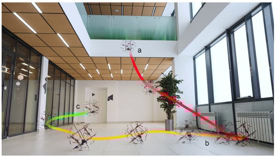
Figure 1.
Tensodrone: a tensegrity-based quadrotor UAV; (a) flight, (b) crash landing, and (c) take-off.
In this work, one additional advantage of using tensegrity structures for drone body design is explored: the possibility to control their shape by actuating one of the structural elements (one of the cables or struts). Through this, the drone can change its shape mid-flight in order to fit through narrow openings, lower the risks of collisions, or change the apparent stiffness of the structure. This concept has been discussed in a previous work [12], where the deformation of a drone was planned as a series of semidefinite programs (SDPs); in particular, a sequence of deformations of a bounding volume was planned and then mapped to actual configurations using a dataset with precomputed bounding volumes and their Eigendecompositions. The proposed approach required an assumption that the change in the robot’s shape as it goes through a deformation can be accurately described by a positive-semidefinite matrix. This excludes non-linear deformations. Here, we propose a mixed-integer planning method that allows the simultaneously planning of the path of the robot and the selection of a configuration for each path point; configuration is a statically stable shape of the tensegrity structure, given the current state of the actuated structural elements. The resulting problem is a mixed-integer quadratic program (MIQP), which can be solved with a branch-and-bound method. This representation is of special interest in the cases when only a limited discrete set of configurations is expected to occur; for instance, if only two rods are actuated in order to control one of the dimensions of the robot and the range of deformations is divided into N discrete configurations. In the paper, an analysis of the impact of the change in the number of integer variables on the performance of the proposed algorithm is given.
Thus, the overall contribution of the work is two-fold: (1) a tensegrity-based drone design and a working prototype, and (2) a path deformation-enabled planning method cast as a mixed-integer quadratic problem, which dismisses one of the assumptions the previously proposed method required. The rest of the paper is organized as follows. Section 2 contains discussion of the state of the art. Section 3 describes the problem to be solved, including the discussion of static equilibrium conditions of tensegrity structures, the mathematical description of obstacle-free areas, and path planning as a mixed-integer problem. Section 4 describes configuration dataset generation. Section 5 outlines the proposed algorithm for simultaneously planning the path and the sequence of deformations, Section 6 gives results of the numerical studies, and Section 7 describes physical experiments performed with the drone prototypes.
2. State of the Art
2.1. Protective Cage Design for Drones
One of the important problems in drone mechanical design has been ensuring human safety in human–robot interactions and robot safety in collisions with the environment. In both cases, an emphasis has been put on preventing propeller blades from making contact interactions with objects in the environment; additionally, prevention of mechanical damage to the robot frame in the event of crash landing has been considered [3,13,14]. The most popular approach in both cases is the use of protective cages. In [15], a protective cage based on Euler springs was studied. In [3], a foldable origami-inspired cage was proposed, with the goal of providing sufficient space for cargo, while the drone itself is easy to transport in the folded form. In [16], an HVAC ducts inspection drone with a rigid cage was proposed; the cage design facilitated both hovering and rolling motion.
In general, advancements in drone protective cage design aimed for some or all of the following goals: (1) lower weight, (2) comprehensive drone and cargo protection, (3) foldability and ease of transportation, and (4) additional maneuverability. The use of tensegrity structures in place of rigid robot frames can potentially lead to lowering the weight of the robot (tensegrity structures are known for good mass-to-stiffness ratios [7]), making the robots foldable in no pre-stress state [3], and facilitating mid-flight morphing [12]. Note that there have been works on using tensegrity structures in drone protective cage design [17]; however, the drones in question still used traditional rigid frames.
2.2. Mechanical Design of Tensegrity Structures
The design of tensegrity structures has been studied since the seminal work of Snelson and Fuller in the 1940s and 1950s. A number of well-behaved tensegrity structures, such as tensegrity prisms and towers, various symmetrical sphere-like structures, and tensegrity trusses have been proposed and studied [18,19,20]. One of such structures is the six-bar tensegrity structure, most notably used in the design of NASA’s planetary probe prototype SUPERBall [21,22,23]. Simulation and experiments with the prototype demonstrated its ability to withstand impact without mechanical damage, as well as its ability to move by rolling, using controlled deformation of the structure to change the relative position of its center of mass.
The design of new tensegrity structures can be done in a variety of ways, including combinations of known structures and direct topology optimization [24,25]. Once the topology of the structure (which element is connected to which) is known, configuration (position of structs and cables) and pre-stress (defined by rest lengths of the deformable elements) need to be determined [26]. A configuration with a given pre-stress is statically stable if it corresponds to a local minimum in potential energy of the structure. Given different rest lengths of deformable elements, a different configuration would correspond to a local minimum in potential energy. Thus, by changing the rest lengths of deformable elements, one can control the shape of the structure. The task of finding force distribution that proves that the configuration corresponds to a local minimum of potential energy can be solved in a number of ways, including the force density method [27,28]. The task of finding a statically stable configuration, given rest lengths of deformable elements, can be solved as a nonlinear optimization problem [29].
In this work, a six-bar tensegrity structure is used to build the world’s first tensegrity drone (referring to the drone’s frame structure; the first drone to use tensegrity as a protective shield, to the best of our knowledge, was reported in [17]). A dataset of stable configurations is generated using energy minimization cast as a single nonlinear optimization problem, as proposed in [29], using different rest lengths of the deformable elements to generate different configurations.
2.3. Deformation-Enabled Path Planning
In the previous work, a method for simultaneously planning a path and sequence of deformations for a tensegrity drone, cast as a sequence of semidefinite programs (SDP), was introduced [12]. If one of many possible paths needs to be chosen, the program will need to take the form of a mixed-integer optimization. A major practical limitation of the proposed approach was the assumption that the shape of the tensegrity structure (and its deformation) can be represented as a positive-definite matrix, allowing the planning if a sequence of deformations as a sequence of covering ellipsoids, which can then be mapped back to actual configurations. Here this assumption is lifted; the algorithm instead works directly with tensegrity configurations. The algorithm proposed in this paper can directly plan a path while choosing a sequence of configurations, as a single mixed-integer quadratic problem. Quadratic problems are known to be easier to solve numerically than SDPs. In both cases, the introduction of integer variables requires an iterative solving procedure based on branch and bound methods, which are in general computationally hard. However, if choosing one path out of multiple available ones is required, the ability to cast the problem as mixed-integer quadratic rather than a mixed-integer semidefinite gives a clear advantage. The limitations of the method are demonstrated via numerical studies in the later parts of the paper.
2.4. Motion Planning for Rigid Drones
UAV route planning has been done in a variety of ways, using methods such as the Voronoi diagram approach, rapidly-exploring random trees algorithm, evolutionary algorithm, particle swarm optimization, D* algorithm, vector field histogram algorithm, dynamic window technique, and artificial potential fields method [30,31,32,33,34]. Recent studies have focused on combining the static programming algorithm for global path planning with the dynamic path search algorithm for local path planning, as well as the aircraft’s kinetic or dynamic constraints, to make the path feasible for a drone to track under specified performance conditions.
In B. T. Lopez and S. LaValle’s work, dynamic path planners employ a memory-less representation of the environment, and closed-form primitives are used for planning [35,36]. In complicated, cluttered environments, these tactics can fail. Map-based static planners, on the other hand, often depict the environment with occupancy grids or distance fields. These planners may either plan the entire trajectory at once or use a Receding Horizon Planning Framework to optimize trajectories locally while still using a global planner. In [37,38] so-called optimistic planners (assuming unknown space to be free) are employed, whereas in the work [39], an optimistic global planner is paired with a conservative local planner.
In [40] a planning framework that uses multi-fidelity models to bridge the gap between local and global planners is suggested. They consider sensor data not yet fused into the map during the collision check to address the relationship between a fast planner and a slower mapper [40]. A FASTER (Fast and Safe Trajectory Planner) is proposed to achieve agile flying in unknown crowded surroundings with high velocity. Their work also uses mixed-integer quadratic program formulation for further performance improvements.
The study [41] makes use of the KD-tree fast nearest neighbor search characteristic and constructs a flight corridor with a safety guarantee in 3D space using a sampling-based path-finding algorithm based on an incrementally built point cloud map. They employ a quadratically constrained quadratic programming (QCQP)-based trajectory generating method to construct trajectories that are totally limited within the corridor [41].
2.5. Convex and Mixed Integer Optimization in Motion Planning
The use of mixed-integer formulations in path planning is not new; it has been done in ariel, underwater, and walking robotics, to name a few examples [42]. Convex solvers are much faster than general non-linear optimization algorithms; however, casting a path-planning problem as convex severely restricts the possible scenarios the planner can tackle. The use of mixed-integer variables here lifts some of these restrictions, most notably restrictions on the convexity of the obstacle-free area, but also restrictions on the types of movements the robot can make. Thus, in [43], the authors developed a mixed-integer footstep planning method, eliminating the problem of non-convex rotation-related constraints by replacing them with mixed-integer piece-wise linear ones.
Additionally, a sequence of convex optimizations can be used to generate free space segmentation into large overlapping obstacle-free convex regions. In [44], the free space segmentation algorithm IRIS (Iterative Regional Inflation by Semi-definite Programming) was proposed; it represented a new approach for calculating large polytopic and ellipsoidal regions of obstacle-free space efficiently via a sequence of convex optimizations.
Here, mixed-integer optimization is adopted for simultaneous path planning and deformation planning of a tensegrity drone, which has not been previously reported in the literature.
3. Problem Statement
3.1. Static Equilibrium of Tensegrity Structures
Tensegrity structures consist of elements experiencing tensile forces, called cables, and of elements bearing compressive forces, called struts. In a pure tensegrity structure, a strut is only connected to cables at two points, referred to as nodes. A straight-forward way to model the system is to model each strut as a rigid body with a given mass and inertial matrix, and cables as massless springs. However, several simplifications can be used to streamline modeling of the static equilibrium of the structure. One of the often-employed simplifications is the assumption that the structure can be equivalently modeled as a set of massive point-like nodes, connected via massless springs. The mass of the structure is thus lumped at the nodes and the external forces are assumed to act on the nodes directly. This assumption is justified when the resulting model is used primarily to compute the shape of the configuration of the tensegrity structure under a given pre-stress, when the magnitudes of the tensile and compressive forces are significantly higher than those of other forces acting on the structure.
Thus, one of the ways to mathematically describe the static equilibrium of a tensegrity structure is by considering the static equilibrium of each node independently. Let the tensegrity structure consist of n nodes, with the i-th node’s position specified by a vector . The topology of the structure is given by a symmetric connectivity matrix with binary elements; if , then the i-th node is connected with the j-th node .
where is the force acting from the i-th node to the j-th node and is the sum of external forces acting on the i-th node. Assuming the linear elastic force equation, can be modeled as:
where is a linear stiffness coefficient and is the elastic element’s rest length: the distance between and when they do not exert force onto each other. The relation between the stiffness coefficient and connectivity matrix is given by the following complementary constraint:
Equations described in this section can be used to study two related questions: (1) whether or not a given configuration (as described by positions of the nodes ) is in static equilibrium for a given pre-stress (as described by the values of ) and (2) what the closest static equilibrium configuration is to a given one, for a given pre-stress. The first question can be answered by checking that condition (2). The second can be solved by finding the minimum potential energy of the structure and fixing its center of mass at the origin. Note that this leads to a family of solutions, as rotation of the structure does not change potential energy.
3.2. Obstacle-Free Space Description
Assume that the drone is moving through an obstacle-free non-convex path-connected space in . This space can be approximated as set of convex polytopes; algorithms for generating such polytopes are described in [44,45,46]. Each such polytope can be represented using H-representation:
If the drone is represented as a set of nodes , then one can check if the drone is located in a polytope using the following condition:
We will refer to this as the region-fit constraint.
3.3. Path Planning as a Mixed-Integer Convex Program
Assume a drone is required to find a path from point to point in K steps while remaining inside obstacle-free space. This implies that for any step , the robot needs to be inside at least one of the polytopes . Problems of this class can be solved using the mixed-integer formulation, and the big-M method in particular [47].
Given binary variables , the region-fit constraint in the optimization problem described above can be written as follows:
where is the position of the center of mass of the structure on the k-th step, T is the number of polytopes , and M is a large scalar constant, chosen such that holds for all in the admissible range.
Note that the use of big-M relaxation increases the number of constraints for each step from n to , where n is the number of nodes in the structure.
4. Configurations Dataset
Our approach to path planning is based on discretizing the path into K steps and directly searching for an appropriate configuration at each step. This requires a dataset of configurations that can be achieved by the robot. An assumption is made that the admissible configurations are only the ones where the tensegrity structure is in static equilibrium.
4.1. Configuration Vector
To represent a configuration in a compact manner, a configuration vector describing the positions of all nodes of the structure is introduced:
where n is the number of nodes in the structure. To retrieve the position of an individual node from the configuration vector, indexing matrices are used:
A number of different configuration vectors form a configuration dataset. Different configurations in the dataset are numbered with upper scripts, with q-th configuration in the dataset represented as . The total number of configurations in a dataset is denoted as Q.
With that, the test whether or not a configuration lies inside a polytope takes the form:
Conditions of static equilibrium can be re-formulated in a similar manner. Note that in practical development, the indexing can be implemented by reshaping the vector into a array, which can be indexed using standard matrix indexing operators; this negates the need for matrix multiplication in (8) and thus should be done when possible.
4.2. Dataset Generation
The proposed algorithm (described in the following section) requires a dataset of admissible configurations. As mentioned in the previous section, a configuration can be generated by choosing and finding th corresponding , which finds a minimum potential energy of the structure. This can be directly replicated in an experimental study by choosing elastic elements with a given (which in practice means changing cable lengths or strut lengths) and recording steady-state positions of the nodes.
In order to generate the configuration dataset, one must establish which elements of are going to change. The indexes of the elements of that change are stored in a vector , meaning that it is elements ,..., that are changing, while the rest remain static. We define a vector of changing rest lengths :
Additionally, we define projector matrices and , such that the following holds:
Then, given the value of and a set of values of , one can find a corresponding , and hence the corresponding configuration vector .
Algorithm 1 performs generation of a configuration dataset based on the process described above. In the Algorithm 1, is the vector of default rest length values for the elastic elements in the tensegrity structure, is the set of all admissible values of (changing rest lengths of the elastic elements), is the potential energy of the structure, is a small regularization coefficient, and is the configuration vector that corresponds to the static equilibrium for the structure given by the vector of default rest lengths . Note that minimization in is understood as the result of applying gradient descent from the initial guess .
| Algorithm 1 Configurations dataset generation algorithm |
Input: , , Output: Dataset whiledo end while |
5. Mixed-Integer Convex Path and Morphing Planner
In this section, a path and morphing planner cast as a single mixed-integer convex program is described. The main difference between the proposed approach and the traditionally employed method for path planning over a union of convex regions is the introduction of another set of choices related to the shape of the robot. The fact that the shape of the robot appears as a linear term in the constraints (6) allows the use of a big-M type mixed-integer selector, similar to the convex region selector. This requires writing a region-fit constraint for each node, each configuration, each possible region, and each step. The resulting optimization problem is given below:
where Q is the number of configurations, K is the number of steps, is the desired starting position of the center of mass of the structure, is the desired end position of the center of mass, is the vector of the same dimensions as whose elements are all ones, and w is a weight-adjusting relative importance of our primary objective (starting from the point and finishing at the point ) and our secondary objective (making the footsteps evenly spaced). Furthermore, note that ; ; ; .
The use of big-M relaxation leads to constraints and binary variables. Binary variables only appear in the constraints, which they enter linearly. The constraints are linear equalities and inequalities; the objective is quadratic, meaning that the proposed problem is a mixed-integer quadratic program. Problems of this type can be solved with Gurobi and MOSEK commercial solvers, among others [48]. Let us note that the number of solvers that handle mixed-integer quadratic problems is greater than for more general case mixed-integer convex optimization problems [48].
6. Numerical Studies, Results
In this section, the numerical studies performed in order to verify the proposed algorithm are outlined, and its numerical properties are analyzed. The study is divided into two parts: (1) demonstration of the feasibility of the approach where a single path planning problem is solved and (2) gathering and analyzing solver statistics by solving a set of problems with small parameter perturbations.
6.1. Planning Drone Path and Deformation through a Series of Rooms
In this section, the results of numerical studies of the algorithm are discussed. As stated previously, this requires generation of a configuration dataset, which in turn requires choosing an actuation pattern: which of the elastic elements are changing their lengths and which do not. We consider the case when only two vertical struts are changing their lengths. This is illustrated in the Figure 2.
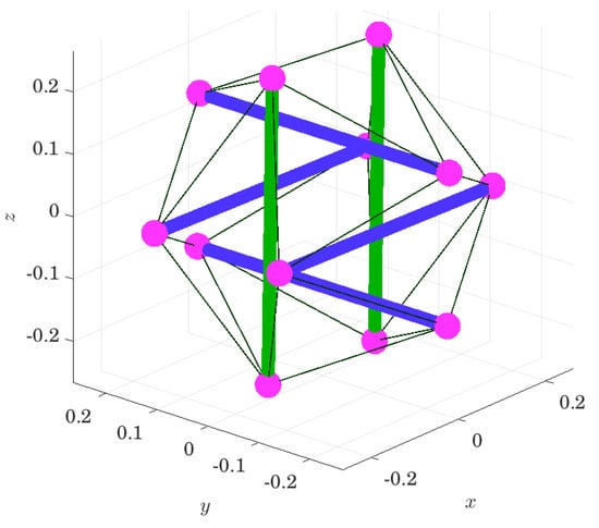
Figure 2.
Actuation pattern on the tensegrity drone; static rest length struts are drawn in blue, the actuated struts in green, the nodes in magenta, and the cables in black.
Consider the following experiment. Given three rooms: room A, room C, and room E, with rooms A and C connected via a narrow tilted shaft B, and rooms C and E connected via a narrow tilted shaft D; the robot needs to plan a path from the center of room A to the center of room E. Each room is 4.5 by 3 by 3.5 m, shaft B is 0.5 m wide, and shaft D is 0.7 m wide, with a slope of 45 degrees. For this task, the rooms A, C, and E are represented as H-polytopes , , and , and the corridors B and D are represented as H-polytopes and . The drone is based on the six-bar tensegrity structure and has 12 nodes. The rooms are modeled as rectangles, giving six linear inequalities describing each room. The configuration dataset used has eight elements.
Two experiments are run: (1) 27 steps are allocated for the path from the starting point to the goal and (2) only 5 steps are allocated for the path. Both problems are solved using (13); the problems are written in CVX, using Gurobi 9.0 as a solver. In the first case, before simplifications, 351 binary variables and 77,760 scalar linear inequalities are expected, while in the second case, only 65 binary variables and 14,400 linear inequalities are expected. The problem was solved on a i7-9700K CPU, 3.60GHz with 32 Gb RAM. Figure 3 gives a pictorial representation of a plan with 27 steps. The details of these two experiments are given in the Table 1.
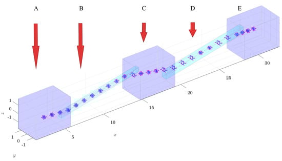
Figure 3.
Path and sequence of deformation planned with the proposed method; A, C and E are rooms, and B and D are corridors.

Table 1.
Parameters of the six-bar tensegrity drone path and morphing planning through three rooms connected via tilted shafts, with 5- and 27-step paths.
Let us observe that while both methods found solutions, the 27-step case took 733 s, while the 5-step case required only 2.8 s. These results depend on the solver settings; here, the Gurobi gap value of 0.05 is used. Notice that while 27 steps required a prohibitively long time, necessitating that the computations be done offline, the 5-step path was computed essentially in real time. In practice, one does not expect to compute long paths spanning more than two rooms, making this experiment more demanding than an average use case. Furthermore, the increase in time between cases is not linear, while the increase in the number of decision variables and constraints is. This is a natural consequence of the combinatorial nature of the branch and bound algorithm and mixed-integer programs. The next subsection gives a study of parameter and time-cost growth as the planned paths become longer, taking into account the solver settings.
6.2. Study of the Computational Cost of the Algorithm
In this section, the study of how the time cost and the number of variables depend on the “path length” (as given by the number of steps between the start and the finish points) is undertaken. The same problem as described in the above subsection is considered and solved for a varying number of steps K.
The following experimental design is used. To collect a single data point, choose K in the range of 3 to 27, and solve Equation (13); this is repeated 10 times and the averages and the range of results are recorded. Repeat this procedure for three different values of the Gurobi gap parameter—0.05, 0.02, and 0.005—recording the results for each value individually; the effect this parameter has on the results is discussed below. The following dependencies are plotted: CPU time as a function of K (Figure 4), number of iterations as a function of K (Figure 5), and number of variables as a function of K (Figure 6).
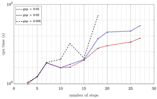
Figure 4.
CPU time as a function of the number of steps, calculated for Gurobi gap values 0.05, 0.02 and 0.005; vertical axis is given in logarithmic scale.
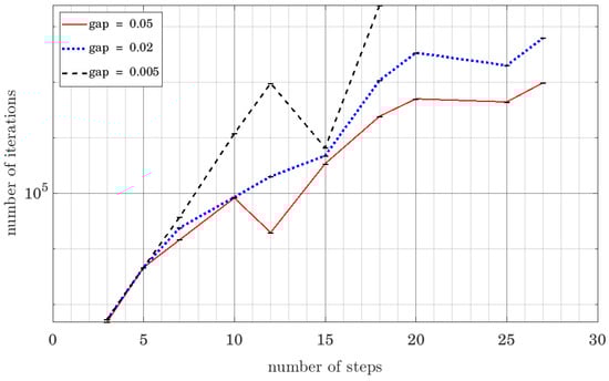
Figure 5.
Number of iterations as a function of the number of steps, calculated for Gurobi gap values 0.05, 0.02 and 0.005; vertical axis is given in logarithmic scale.
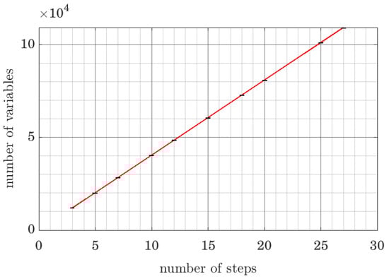
Figure 6.
Number of optimization variables after simplification as a function of the number of steps.
From Figure 5, one can observe a rapid growth in the number of iterations for all values of the Gurobi gap; however, when gap 0.005 is chosen, the growth becomes exponential, appearing linear in the semilog scale. This mainly indicates the necessity of choosing the Gurobi gap carefully when solving the problem (13), as the choice can easily render the problem practically intractable. Figure 4 shows close correspondence with Figure 5, which is to be expected if each iteration takes roughly the same time. In both cases, one can note that the difference between choosing the Gurobi gap to be 0.05 or 0.02 plays a significant role in the performance only for longer paths (more than 15 steps), while for shorter paths, the difference is small. This is a good indicator that the algorithm’s performance is robust to small changes in this parameter, which is important for its practical usefulness. Note that at 15 steps, the solution takes 30 and 32.5 s for gap values 0.02 and 0.05, respectively. Finally, from Figure 6, one can observe that the number of variables after simplification (as performed by CVX) grows linearly with the number of steps, which is to be expected, as the constraints associated with each step are independent of each other in terms of both the binary and continuous variables that enter them.
Note that all graphs in Figure 4, Figure 5 and Figure 6 have error bars, but these are too tight to be distinct, indicating that, at least within this experimental design, the results are replicable. However, it would be of additional interest to repeat the same experiment, but using a sufficiently large dataset of locations, which would correspond to typical use cases for such drones.
7. Experimental Study
In this section, the feasibility of the proposed concept is considered. Two designs of tensegrity drones (drones whose frame is a tensegrity structure) are presented, which are the first designs to be reported in the literature.
7.1. Pure Tensegrity Drone
This subsection presents Tensodrone: a drone whose frame is a six-bar tensegrity structure. The drone is propelled with four motors and is controlled via a PX4 flight controller. Figure 7 shows the photo of the Tensodrone with annotations. Previously in Figure 1, a Tensodrone flight experiment were demonstrated, where the Tensodrone took off, flew, intentionally performed a crashlanding, and then took off again, this time with human assistance. This is possible due to the discussed previously properties of tensegrity structures (their resilience to impact) and also because of the geometry of the Tensodrone frame, which makes it possible to use motors to change drone’s orientation when it is on the ground and to make the drone “face up” and take off. Mechanical parameters of the drone are given in Table 2.
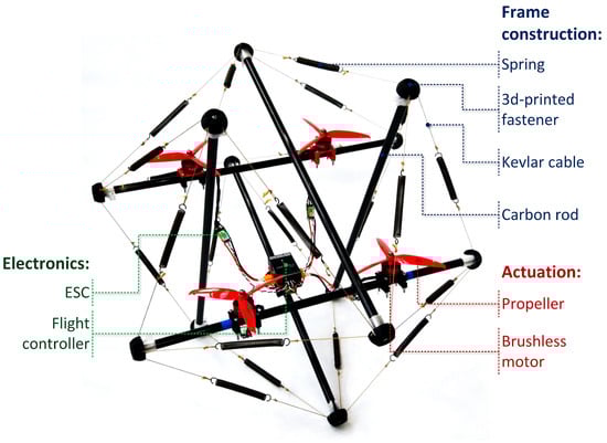
Figure 7.
Pure tensegrity drone; ESC stands for Electronic Speed Controller; the flight controller used is PX4.
Table 2.
Mechanical parameters of the Tensodrone prototype.
In the proposed tensegrity drone design, any strut can be replaced with lightweight linear drives, implementing in-flight morphing. Our experiments with the design of lightweight linear drives were focused on twisted string actuator-based models, using the design studied in [49]. In this study, the experiments are limited to standard flight controllers, facilitating comparison with traditional rigid-frame drone design. Standard flight controllers neither take into account the oscillatory motion of the drone struts relative to one another, nor compensate for the orientation estimation errors cause by those vibrations, making the experimental study results dependent on the stiffness of the elastic elements used in the tensegrity drone design and, in general, on the stiffness matrix of the structure. This motivated a second generation tensegrity drone design, shown in the next subsection.
7.2. Tensegrity Drone with Strut Contact
In order to improve the performance of the drone and to make the structure more compact, an additional horizontal strut was added, making the drone frame a seven-bar tensegrity. The levels of pre-stress were increased, leading to struts touching each other, making the structure transcend the definition of pure tensegrity, as the struts in this case can experience forces other than pure compression. The design of the drone and an in-flight photo are shown in Figure 8.
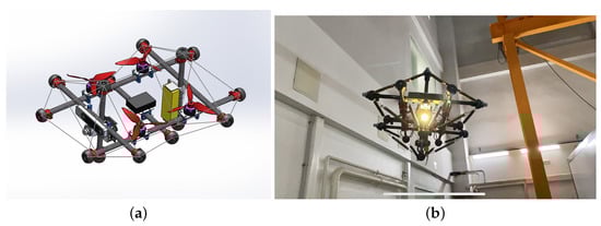
Figure 8.
Second generation tensegrity drone. (a) CAD model. (b) In-flight photo.
The following series of experiments was conducted. The second generation tensegrity drone and a rigid-frame drone QAV-R 5″ Racer were outfitted with visual markers designed to work with the motion capture system OptiTrack. Both drones were required to fly over a pre-determined 8-shaped trajectory and their flight parameters were logged using PX4 measurement and logging solution, processed via Flight Review software. Figure 9 shows the trajectories of the rigid-frame QAV-R 5" Racer and tensegrity drones; the accuracy of the motion capture system measurements is 0.3 mm. Analyzing the graphs, one can note the less consistent behavior of the tensegrity drone as compared with the rigid-body drone; however, it needs to be taken into account that the flight controller used in both experiments was designed for rigid-frame drones. This includes the way the control actions are computed and the way the state of the drone is estimated. The video recordings of the experiments are publicly available: flight tests for tensegrity and rigid-frame drones: https://youtu.be/X8SFrV3l4A8 (accessed on 30 April 2022), https://youtu.be/LxREx53Sna8 (accessed on 30 April 2022).
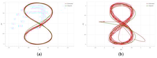
Figure 9.
Drone trajectory captured by the visual motion capture system OptiTrack in the horizontal plane. (a) Rigid-frame drone QAV-R Racer. (b) Second-generation tensegrity drone.
The same experiments were used to produce spectra of acceleration power spectral density for both the rigid-frame drone QAV-R Racer (see Figure 10) and the tensegrity drone (see Figure 11). The measurements were performed using CUAV PX4 V5 nano board with IMUs ICM-20689, ICM-20602, and BMI055; their readings were combined in an extended Kalman filter, implemented in PX4 software. As can be seen in the spectra, the rigid drone exhibits a band of higher accelerations at higher frequencies compared to the tensegrity drone. The tensegrity drone, on the other hand, exhibits a clear dominant frequency that remains stable throughout the whole experiment. The amount of lower frequency accelerations for the tensegrity drone is higher than for a rigid-frame drone, as could be expected based on the presence of the elastic elements.
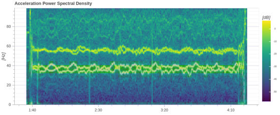
Figure 10.
Spectrum for a rigid-frame drone QAV-R Racer collected via PX4 log collector and plotted using PX4 Flight Review.
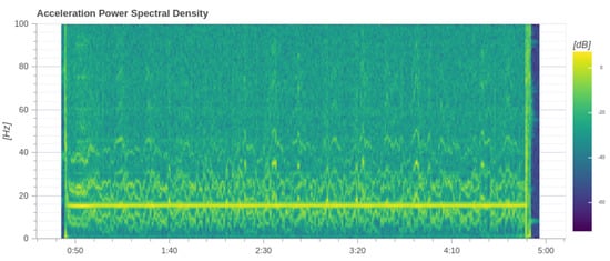
Figure 11.
Spectrum for the second-generation tensegrity drone collected via PX4 log collector and plotted using PX4 Flight Review.
8. Discussion
In this paper, a new type of drone design based on tensegrity structures was discussed. This design allows the drones to withstand collisions, as was demonstrated in experimental studies. Actuating one or more of the structural elements (in particular, making the rest lengths of the elastic elements change) makes it possible to reshape the structure, as has been demonstrated before in tensegrity planetary lander designs, for instance. A mixed-integer method for simultaneously planning a path and producing a sequence of deformations was proposed, making it possible for the robot to fit through narrow gaps, corridors, and shafts when navigating through a cluttered environment. The proposed algorithm scales with the number of steps, however a proper cut-off value for the algorithm termination (such as Gurobi gap parameter) needs to be chosen to avoid exponential growth in the computational time at higher numbers of steps. In the example with five obstacle-free areas (three rooms connected via two tilted shafts), it was found that paths up to 15 steps can be found under 32 s, while 5-step paths require less than 3 s of CPU time. The main advantage of the proposed method compared with the previous one is qualitative rather than quantitative: casting the problem as a mixed-integer quadratic instead of mixed-integer semidefinite program makes it possible to use a much wider range of solvers, effectively relaxing the requirements on the software needed to support the motion planning.
Two prototypes of tensegrity drones were demonstrated and tested: a six-bar pure tensegrity drone and a seven-bar higher pre-stress design. Both were tested for collision resilience, and motion capture and on-board logging were used to study the trajectory and frame vibrations of the seven-bar drone design in comparison with a rigid-body QAV-R Racer. Both drones performed, but with different distributions of frame vibration frequencies, with more pronounced and lower dominant frequencies for the tensegrity drone.
Future work on tensegrity drones can take two directions: (1) optimal mechanical design of the drones and (2) state estimation and control design, taking into account the dynamic behavior of tensegrity frames.
Author Contributions
Conceptualization, S.S. and A.K.; methodology, S.S. and R.F.; software, S.S. and A.A.B.; validation, A.A.B., D.D., and R.F.; formal analysis, S.S. and A.A.B.; investigation, S.S., A.A.B., D.D., and R.F.; resources, S.S., R.F., and A.K.; data curation, S.S., D.D., and R.F.; writing—original draft preparation, S.S., A.A.B., and A.K.; writing—review and editing, S.S. and A.K.; visualization, S.S. and A.A.B.; supervision, S.S. and A.K.; project administration, S.S., R.F. and A.K.; funding acquisition, S.S. and R.F. All authors have read and agreed to the published version of the manuscript.
Funding
This research is supported by a grant from the Russian Science Foundation (project No:19-79-10246).
Institutional Review Board Statement
Not applicable.
Informed Consent Statement
Not applicable.
Acknowledgments
We are thankful to Igor Gaponov for his advice during the design and early experimentation with tensegrity drone prototypes. We are also thankful to Vladimir Antipov and Oleg Balahknov for their involvement in the assembly and tests of the original tensegrity drone prototype, as well as to Hany Hamed for his help with the experiments.
Conflicts of Interest
The authors declare no conflict of interest.
Abbreviations
The following abbreviations are used in this manuscript:
| MICP | Mixed-Integer Convex Programming |
| IRIS | Iterative Regional Inflation by Semi-definite programming |
| SDPs | Semidefinite Programs |
| MIQP | Mixed-Integer Quadratic Program |
| UAV | Unmanned Aerial Vehicle |
| HVAC | Heating, Ventilation, and Air-Conditioning |
| RRT | Rapidly Exploring Random Tree |
| QCQP | Quadratically Constrained Quadratic Programming |
| MIP | Mixed-Integer Programming |
References
- Kardasz, P.; Doskocz, J.; Hejduk, M.; Wiejkut, P.; Zarzycki, H. Drones and possibilities of their using. J. Civ. Environ. Eng. 2016, 6, 1–7. [Google Scholar] [CrossRef]
- Edgerton, K.; Throneberry, G.; Takeshita, A.; Hocut, C.; Shu, F.; Abdelkefi, A. Numerical and experimental comparative performance analysis of emerging spherical-caged drones. Aerosp. Sci. Technol. 2019, 95, 105512. [Google Scholar] [CrossRef]
- Kornatowski, P.M.; Mintchev, S.; Floreano, D. An origami-inspired cargo drone. In Proceedings of the 2017 IEEE/RSJ International Conference on Intelligent Robots and Systems (IROS), Vancouver, BC, Canada, 24–28 September 2017; pp. 6855–6862. [Google Scholar]
- Chen, C.S.; Ingber, D.E. Tensegrity and mechanoregulation: From skeleton to cytoskeleton. Osteoarthr. Cartil. 1999, 7, 81–94. [Google Scholar] [CrossRef] [PubMed] [Green Version]
- Motro, R. Tensegrity: Structural Systems for the Future; Elsevier: Amsterdam, The Netherlands, 2003. [Google Scholar]
- Skelton, R.E.; Adhikari, R.; Pinaud, J.P.; Chan, W.; Helton, J. An introduction to the mechanics of tensegrity structures. In Proceedings of the 40th IEEE Conference on Decision and Control (Cat. No. 01CH37228), Orlando, FL, USA, 4–7 December 2001; Volume 5, pp. 4254–4259. [Google Scholar]
- Moored, K.; Kemp, T.; Houle, N.E.; Bart-Smith, H. Analytical predictions, optimization, and design of a tensegrity-based artificial pectoral fin. Int. J. Solids Struct. 2011, 48, 3142–3159. [Google Scholar] [CrossRef] [Green Version]
- Jáuregui, V.G. Tensegrity Structures and Their Application to Architecture; Universidad de Cantabria: Santander, Spain, 2020; Volume 2. [Google Scholar]
- Bouderbala, M.; Motro, R. Folding tensegrity systems. In Proceedings of the IUTAM-IASS Symposium on Deployable Structures: Theory and Applications; Springer: Berlin/Heidelberg, Germany, 2000; pp. 27–36. [Google Scholar]
- Vespignani, M.; Friesen, J.M.; SunSpiral, V.; Bruce, J. Design of superball v2, a compliant tensegrity robot for absorbing large impacts. In Proceedings of the 2018 IEEE/RSJ International Conference on Intelligent Robots and Systems (IROS), Madrid, Spain, 1–5 October 2018; pp. 2865–2871. [Google Scholar]
- Caluwaerts, K.; Despraz, J.; Işçen, A.; Sabelhaus, A.P.; Bruce, J.; Schrauwen, B.; SunSpiral, V. Design and control of compliant tensegrity robots through simulation and hardware validation. J. R. Soc. Interface 2014, 11, 20140520. [Google Scholar] [CrossRef] [Green Version]
- Savin, S.; Klimchik, A. Morphing-Enabled Path Planning for Flying Tensegrity Robots as a Semidefinite Program. Front. Robot. AI 2022, 9. [Google Scholar] [CrossRef]
- Abtahi, P.; Zhao, D.Y.; E, J.L.; Landay, J.A. Drone near me: Exploring touch-based human-drone interaction. Proc. ACM Interact. Mobile Wearable Ubiquitous Technol. 2017, 1, 1–8. [Google Scholar] [CrossRef] [Green Version]
- Kornatowski, P.M.; Feroskhan, M.; Stewart, W.J.; Floreano, D. A morphing cargo drone for safe flight in proximity of humans. IEEE Robot. Autom. Lett. 2020, 5, 4233–4240. [Google Scholar] [CrossRef]
- Klaptocz, A.; Briod, A.; Daler, L.; Zufferey, J.C.; Floreano, D. Euler spring collision protection for flying robots. In Proceedings of the 2013 IEEE/RSJ International Conference on Intelligent Robots and Systems, Tokyo, Japan, 3–7 November 2013; pp. 1886–1892. [Google Scholar]
- Borik, A.; Kallangodan, A.; Farhat, W.; Abougharib, A.; Jaradat, M.A.; Mukhopadhyay, S.; Abdel-Hafez, M. Caged Quadrotor Drone for Inspection of Central HVAC Ducts. In Proceedings of the 2019 Advances in Science and Engineering Technology International Conferences (ASET), Dubai, United Arab Emirates, 26 March–10 April 2019; pp. 1–7. [Google Scholar]
- Zha, J.; Wu, X.; Kroeger, J.; Perez, N.; Mueller, M.W. A collision-resilient aerial vehicle with icosahedron tensegrity structure. In Proceedings of the 2020 IEEE/RSJ International Conference on Intelligent Robots and Systems (IROS), Las Vegas, NV, USA, 24 October 2020–24 January 2021; pp. 1407–1412. [Google Scholar]
- Sultan, C. Tensegrity: 60 years of art, science, and engineering. Adv. Appl. Mech. 2009, 43, 69–145. [Google Scholar]
- Furuya, H. Concept of deployable tensegrity structures in space application. Int. J. Space Struct. 1992, 7, 143–151. [Google Scholar] [CrossRef]
- de Jager, B.; Skelton, R.E. Stiffness of planar tensegrity truss topologies. Int. J. Solids Struct. 2006, 43, 1308–1330. [Google Scholar] [CrossRef] [Green Version]
- Sabelhaus, A.P.; Bruce, J.; Caluwaerts, K.; Manovi, P.; Firoozi, R.F.; Dobi, S.; Agogino, A.M.; SunSpiral, V. System design and locomotion of SUPERball, an untethered tensegrity robot. In Proceedings of the 2015 IEEE International Conference on Robotics and Automation (ICRA), Seattle, WA, USA, 26–30 May 2015; pp. 2867–2873. [Google Scholar]
- Bruce, J.; Sabelhaus, A.P.; Chen, Y.; Lu, D.; Morse, K.; Milam, S.; Caluwaerts, K.; Agogino, A.M.; SunSpiral, V. SUPERball: Exploring Tensegrities for Planetary Probes. 2014. Available online: https://ntrs.nasa.gov/api/citations/20190001649/downloads/20190001649.pdf (accessed on 30 April 2022).
- Sabelhaus, A.P.; Bruce, J.; Caluwaerts, K.; Chen, Y.; Lu, D.; Liu, Y.; Agogino, A.K.; SunSpiral, V.; Agogino, A.M. Hardware Design and Testing of SUPERball, a Modular Tensegrity Robot. 2014. Available online: https://ntrs.nasa.gov/api/citations/20140011157/downloads/20140011157.pdf, (accessed on 30 April 2022).
- Lee, S.; Lee, J. A novel method for topology design of tensegrity structures. Compos. Struct. 2016, 152, 11–19. [Google Scholar] [CrossRef]
- Khafizov, R.; Savin, S. Length-Constrained Mixed-Integer Convex Programming-based Generation of Tensegrity Structures. In Proceedings of the 2021 6th IEEE International Conference on Advanced Robotics and Mechatronics (ICARM), Chongqing, China, 3–5 July 2021; pp. 125–131. [Google Scholar]
- Murakami, H. Static and dynamic analyses of tensegrity structures. Part II. Quasi-static analysis. Int. J. Solids Struct. 2001, 38, 3615–3629. [Google Scholar] [CrossRef]
- Xu, X.; Wang, Y.; Luo, Y. Finding member connectivities and nodal positions of tensegrity structures based on force density method and mixed integer nonlinear programming. Eng. Struct. 2018, 166, 240–250. [Google Scholar] [CrossRef]
- Zhang, L.Y.; Zhu, S.X.; Li, S.X.; Xu, G.K. Analytical form-finding of tensegrities using determinant of force-density matrix. Compos. Struct. 2018, 189, 87–98. [Google Scholar] [CrossRef]
- Savin, S.; Balakhnov, O.; Klimchik, A. Energy-based local forward and inverse kinematics methods for tensegrity robots. In Proceedings of the 2020 Fourth IEEE International Conference on Robotic Computing (IRC), Taichung, Taiwan, 9–11 November 2020; pp. 280–284. [Google Scholar]
- Park, J.K.; Chung, T.M. Boundary-RRT* algorithm for drone collision avoidance and interleaved path re-planning. J. Inf. Process. Syst. 2020, 16, 1324–1342. [Google Scholar]
- Han, T.; Wu, W.; Huang, C.; Xuan, Y. Path planning of UAV based on Voronoi diagram and DPSO. Procedia Eng. 2012, 29, 4198–4203. [Google Scholar] [CrossRef] [Green Version]
- Pehlivanoglu, Y.V. A new vibrational genetic algorithm enhanced with a Voronoi diagram for path planning of autonomous UAV. Aerosp. Sci. Technol. 2012, 16, 47–55. [Google Scholar] [CrossRef]
- Fu, Z.; Yu, J.; Xie, G.; Chen, Y.; Mao, Y. A heuristic evolutionary algorithm of UAV path planning. Wirel. Commun. Mob. Comput. 2018, 2018, 2851964. [Google Scholar] [CrossRef] [Green Version]
- Niu, X.; Yuan, X.; Zhou, Y.; Fan, H. UAV track planning based on evolution algorithm in embedded system. Microprocess. Microsystems 2020, 75, 103068. [Google Scholar] [CrossRef]
- Lopez, B.T.; How, J.P. Aggressive 3-D collision avoidance for high-speed navigation. In Proceedings of the 2017 IEEE International Conference on Robotics and Automation (ICRA), Singapore, 29 May–3 June 2017; pp. 5759–5765. [Google Scholar]
- LaValle, S.M.; Kuffner, J.J., Jr. Randomized kinodynamic planning. Int. J. Robot. Res. 2001, 20, 378–400. [Google Scholar] [CrossRef]
- Pivtoraiko, M.; Mellinger, D.; Kumar, V. Incremental micro-UAV motion replanning for exploring unknown environments. In Proceedings of the 2013 IEEE international conference on robotics and automation, Karlsruhe, Germany, 6–10 May 2013; pp. 2452–2458. [Google Scholar]
- Chen, J.; Liu, T.; Shen, S. Online generation of collision-free trajectories for quadrotor flight in unknown cluttered environments. In Proceedings of the 2016 IEEE International Conference on Robotics and Automation (ICRA), Stockholm, Sweden, 16–21 May 2016; pp. 1476–1483. [Google Scholar]
- Oleynikova, H.; Taylor, Z.; Siegwart, R.; Nieto, J. Safe local exploration for replanning in cluttered unknown environments for microaerial vehicles. IEEE Robot. Autom. Lett. 2018, 3, 1474–1481. [Google Scholar] [CrossRef] [Green Version]
- Tordesillas, J.; Lopez, B.T.; Carter, J.; Ware, J.; How, J.P. Real-time planning with multi-fidelity models for agile flights in unknown environments. In Proceedings of the 2019 international conference on robotics and automation (ICRA), Montreal, QC, Canada, 20–24 May 2019; pp. 725–731. [Google Scholar]
- Gao, F.; Wu, W.; Lin, Y.; Shen, S. Online safe trajectory generation for quadrotors using fast marching method and bernstein basis polynomial. In Proceedings of the 2018 IEEE International Conference on Robotics and Automation (ICRA), Brisbane, Australia, 21–25 May 2018; pp. 344–351. [Google Scholar]
- Yang, L.; Qi, J.; Song, D.; Xiao, J.; Han, J.; Xia, Y. Survey of robot 3D path planning algorithms. J. Control. Sci. Eng. 2016, 2016, 7426913. [Google Scholar] [CrossRef] [Green Version]
- Deits, R.; Tedrake, R. Footstep planning on uneven terrain with mixed-integer convex optimization. In Proceedings of the 2014 IEEE-RAS International Conference on Humanoid Robots, Madrid, Spain, 18–20 November 2014; pp. 279–286. [Google Scholar]
- Deits, R.; Tedrake, R. Computing Large Convex Regions of Obstacle-Free Space Through Semidefinite Programming. In Proceedings of the Eleventh International Workshop on the Algorithmic Foundations of Robotics, Istanbul, Turkey, 3–5 August 2014; pp. 109–124. [Google Scholar]
- Zhong, X.; Wu, Y.; Wang, D.; Wang, Q.; Xu, C.; Gao, F. Generating large convex polytopes directly on point clouds. arXiv 2020, arXiv:2010.08744. [Google Scholar]
- Savin, S. An algorithm for generating convex obstacle-free regions based on stereographic projection. In Proceedings of the 2017 International Siberian Conference on Control and Communications (SIBCON), Astana, Kazakhstan, 29–30 June 2017; pp. 1–6. [Google Scholar]
- Grossmann, I.E. Review of nonlinear mixed-integer and disjunctive programming techniques. Optim. Eng. 2002, 3, 227–252. [Google Scholar] [CrossRef]
- Anand, R.; Aggarwal, D.; Kumar, V. A comparative analysis of optimization solvers. J. Stat. Manag. Syst. 2017, 20, 623–635. [Google Scholar] [CrossRef]
- Nedelchev, S.; Gaponov, I.; Ryu, J.H. Accurate dynamic modeling of twisted string actuators accounting for string compliance and friction. IEEE Robot. Autom. Lett. 2020, 5, 3438–3443. [Google Scholar] [CrossRef]
Publisher’s Note: MDPI stays neutral with regard to jurisdictional claims in published maps and institutional affiliations. |
© 2022 by the authors. Licensee MDPI, Basel, Switzerland. This article is an open access article distributed under the terms and conditions of the Creative Commons Attribution (CC BY) license (https://creativecommons.org/licenses/by/4.0/).