1. Introduction
Ionospheric scintillation is one of the main concerns for satellite communications, in particular for Global Navigation Satellite Systems (GNSS) and low-frequency Earth observation missions, such as the upcoming P-band synthetic aperture radars and radar sounders. They may affect electromagnetic signals traversing the ionosphere, with rapid fluctuations in the intensity and/or phase of the signal. Several models [
1] have been used in recent decades: Rino–Fremouw (1973) [
2,
3], Aarons (1985) [
4], Franke and Liu (1985) [
5], Iyer et al. (2006) [
6], the WBMOD climatological model [
7], or GISM [
8].
Besides being a problem for satellite communications and Earth observation missions, ionospheric scintillation can also be used as a tool for Earth observation.
A novel technique, first introduced in [
9], and continued in [
10,
11], uses GNSS Reflectometry (GNSS-R) technology to infer ionospheric amplitude scintillation over oceanic regions. This technique allows the creation of ionospheric scintillation maps that could help the calibration and improvement of the currently available models.
In the work presented here, the interaction between the ionosphere and the lithosphere is studied.
The lithosphere is the solid, outermost shell of the Earth, and it is subjected to slow movements. The crust is divided in tectonic plates that can move relative to each other because they lie on top of the viscous, upper part of the mantle. The upper mantle plastic deformations absorb the displacements of the crust on timescales of thousands of years, but the solid crust deforms elastically leading to earthquakes through brittle failure.
In the last decade, several studies revealed some coupling between the lithosphere, the atmosphere, and the ionosphere [
12]. In this study, we will focus on the impact of the lithosphere on the ionosphere. According to [
13,
14,
15,
16,
17,
18,
19], this coupling can be observed during earthquakes, in particular, before, during the so-called earthquake’s preparation period, or immediately after them, with different physical explanations.
When the ionospheric perturbations are observed before the earthquake, one reason for this is the perturbation of the background electric field by an electric potential appearing on the Earth’s surface during the earthquake’s preparation period [
14]. For example, microfractures near the epicenter can generate positively charged holes that can diffuse to the surface, and generate these electric fields, that in the end, disturb the ionosphere.
Furthermore, a thermal expansion of the atmosphere derived from the Land Surface Temperature (LST) increase prior to the earthquake occurrence, shown in several studies [
15,
16,
17,
20], can generate a small gravity wave disturbing the electron density profile of the ionosphere, inducing changes in the TEC.
The general interest in this field of study has increased in the last few years, as shown by the dedicated Chinese–Italian mission called China Seismo-Electromagnetic Satellite (CSES) to study the ionosphere-lithosphere coupling by monitoring electromagnetic and plasma density variations in the ionosphere. The satellite was launched to a 500-km altitude polar Sun-synchronous orbit in 2018, and it has already provided some interesting results of TEC variations related to several strong earthquakes in the Indonesian region [
18].
Furthermore, some studies also detected ionospheric perturbations in the hours after large earthquakes, for example in the magnitude 9 Tohoku (Japan) earthquake in 2011. In this case, clear TEC deviations were measured following a concentric wave pattern around the epicenter [
19]. Possible explanations for these perturbations are the acoustic waves generated by the sudden huge mass redistribution produced during the earthquake, that travel to the upper atmospheric layers or the ionosphere, inducing changes in the electron density. These waves can also be generated along the traveling Rayleigh waves propagating concentrically from the epicenter along the Earth’s crust.
Most previous studies on this topic use the TEC anomalous variations as earthquake precursors [
21,
22,
23]. Only a small fraction of the studies on ionospheric perturbations related to earthquakes use ionospheric scintillation to do their correlation [
24]. These studies take GPS data from ground stations [
25], or ground-based ionosondes [
26] to measure the
index and correlate it to earthquakes in the region. The novelty of this study is the use of the GNSS-R technique to obtain global oceanic maps of ionospheric scintillation and correlate them to earthquake precursors, allowing studying a large number of earthquakes globally distributed and making use of statistical tools such as the confusion matrixes and ROC.
Section 2 describes the data used, and the methods applied during this study; it is divided into four subsections.
Section 2.1 describes how ionospheric scintillation is derived from GNSS-R CYGNSS measurements,
Section 2.2 explains how changes in the scintillation index are calculated,
Section 2.3 introduces the earthquake database used, and
Section 2.4 describes how the statistical analysis is performed by means of the confusion matrix method.
Section 3 presents the results of this study, and it is divided into two parts: the first shows the results for a particular case study in July 2019, and the second presents the statistical results of the complete analysis over a period of 6 months from March 2019 to August 2019. Finally, a discussion on the results is performed in
Section 4, and the main conclusions are presented in
Section 5.
2. Materials and Methods
2.1. Ionospheric Scintillation Measurement Using GNSS-R Data
In this study, ionospheric amplitude scintillation (
) data are inferred using GNSS-R products from the NASA Cyclone Global Navigation Satellite System (CYGNSS) mission, following the approach presented in [
9]. This technique computes the scintillation in the signal’s intensity using the following expression:
in which
I is the signal’s intensity or, in our case, the magnitude of the Signal-to-Noise Ratio (SNR) of the Delay-Doppler Map (DDM) of the reflected signal over oceans in linear units, and its average (
) is calculated over a 10 s moving window. This way, global
maps can be elaborated on calm oceanic regions between 40ºS and 40ºN latitudes.
The signals emitted by the GNSS transmitters cross the ionosphere in the down-welling path, then coherently reflect on calm water surfaces, and reach the GNSS-R receiver, in this case, a CYGNSS satellite, which compares the signals with the direct ones. As the signals follow different paths, the reflected ones are more influenced by the ionosphere than the direct ones, therefore the ionospheric scintillation can be detected in the resulting DDM intensity.
The points where the scintillation values are geolocated correspond to the specular reflection point over oceans, which are provided in the CYGNSS L1 dataset. This can be seen as a problem because the actual scintillation is mainly induced at the altitude of the ionosphere, approximately 350 km, near the electron density peak. However, as the reflected signal crosses this layer two times, the middle point between these two pierce points nearly matches the specular reflection point. Furthermore, in later steps, a 100 km radius is used to aggregate data when searching for earthquakes around anomalies in the value, which helps to smooth this effect along with the uncertainty in the distance where earthquakes disturb the ionosphere.
The GNSS-R constellation used, CYGNSS, was originally designed for wind speed and cyclone monitoring. It consists of eight micro-satellites orbiting at around 520 km altitude, with an orbital inclination of 35º. Each satellite can track up to four GNSS signals reflected on the ground [
27], allowing an effective coverage between latitudes −40º to 40º. The constellation was launched in December 2016, and the science data are available from March 2017, with a cadence of 1 DDM per channel per second, resulting in around
samples per day for the whole constellation. The DDM data rate was set to 2 Hz in July 2019.
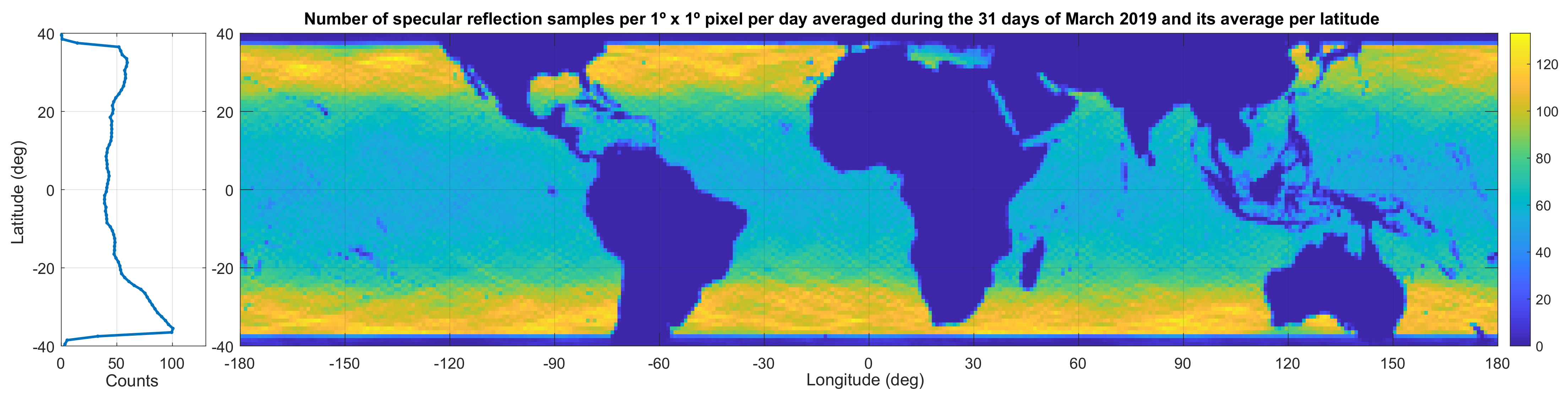
After quality filtering, the total number of samples per day per pixel of
varies from 100 in equatorial regions to 200 in
to 35º North and South, as shown in
Figure 1.
CYGNSS L1 data are filtered out when the “poor_overall_quality” flag is true, which is the union of several flags described in the CYGNSS manual [
27]. The most important flags refer to the land cover filter, which removes all the land points, and the ones that are less than 25 km from the coast. Furthermore, they remove the data when the satellite had suffer from attitude perturbations, or the DDM obtained has low confidence or a large noise figure, or when Radio-Frequency Interference (RFI) has been detected in the measurements.
2.2. Ionospheric Scintillation Changes Computation
Given that ionospheric scintillation is subjected to variations that follow, in the short term, a daily periodicity, and, in the long term, an annual, and 11-year solar cycle trend, data must be detrended to detect anomalous variations. As the daily variations are the short-term larger variations, and also because larger, more random fluctuations due to solar radiation are expected during the daytime, data has been filtered to keep only measurements from 0 h to 6h LT, during the night time, when the ionosphere is expected to be more stable, at least in equatorial regions where this study is conducted. This way we expect to better detect anomalous changes on a time-scale longer than 1 day, which are also more likely to be induced by Earth’s internal sources rather than by solar or space-weather sources.
To detrend the monthly/annual variations, the average of two months has been computed, and then subtracted from a seven day window average, in which we want to compute the
variation. More precisely, for a particular day
D in which the relative variation is computed, the previous 61 day average is subtracted from the previous seven day average (both including the current day
D). This is computed for every day, and every
pixel in the region covered by CYGNSS (from 40ºS to 40ºN) using Equation (
2).
where
represent the longitude and latitude of each pixel in the map, and
d is the day swept to compute the average. The
variation (
) is computed for every day
D, at each pixel in the map. It usually exhibits values ranging
, being positive when the
in the last week has been larger than the typical value during the last two months.
The selection of a two month (61 day) average for detrending is made to remove the long term, annual evolution of the ionospheric activity in addition to the variability of the sea-surface conditions, while the 7 day short average helps to smooth fluctuations in this activity due to space-weather with a daily or weekly timescale, and also fits with the approximate timescales expected for the earthquakes ionospheric precursors to occur, according to the studies referenced in previous sections [
12,
13,
18]. Additionally, both averaging windows are asymmetrical in time, including only values before the current day. The reason for that is that our study is focused on searching for precursory changes in ionospheric scintillation.
Due to the periodicity of the CYGNSS satellite’s orbits, and the filter applied to keep only measurements from 0 h to 6 h LT, a time dependence was observed in the latitude of the regions covered by the study along the period studied.
Figure 2 shows the position of the median latitude of the valid data pixels for every day in the period studied (blue line). It also shows, the area between the first and third interquartiles of the available data pixels (green area), and the maximum and minimum latitudes covered (gray area). This plot shows the oscillating behavior of the region covered in the study.
This variation in the region covered will make that some regions away from the equator would not be included in the study during a certain time. Earthquakes taking place in these periods and regions would not be studied because of the lack of ionospheric scintillation data to correlate with. The method for discarding these data will be explained in the section regarding the creation of the confusion matrix.
2.3. Earthquake Database
The second main data source is composed of the earthquakes database provided by the USGS containing the magnitude, UTC time, depth, and location of the epicenter, among other parameters. It is important to remark that the magnitude is a complex variable to describe, as there are different methods of computation and scales, which depend on the region of the Earth where earthquakes are studied, the composition of the lithosphere, or the measuring technique used.
Originally, the Richter scale (M
l) was developed for earthquakes in the California region by measuring the frequency of the seismic waves received at a seismographic station. Later on, when trying to use the same scale for other regions, it was found that the Richter method was not valid for all frequencies and distance ranges, in particular for larger magnitude earthquakes. Other methods to measure the magnitude were developed, designed to match the Richter scale in their range of validity [
28,
29]. The m
b, using the body wave, and the M
S, using the surface wave are two extensions of the Richter magnitude, but they were not valid for larger earthquakes. The moment magnitude scale M
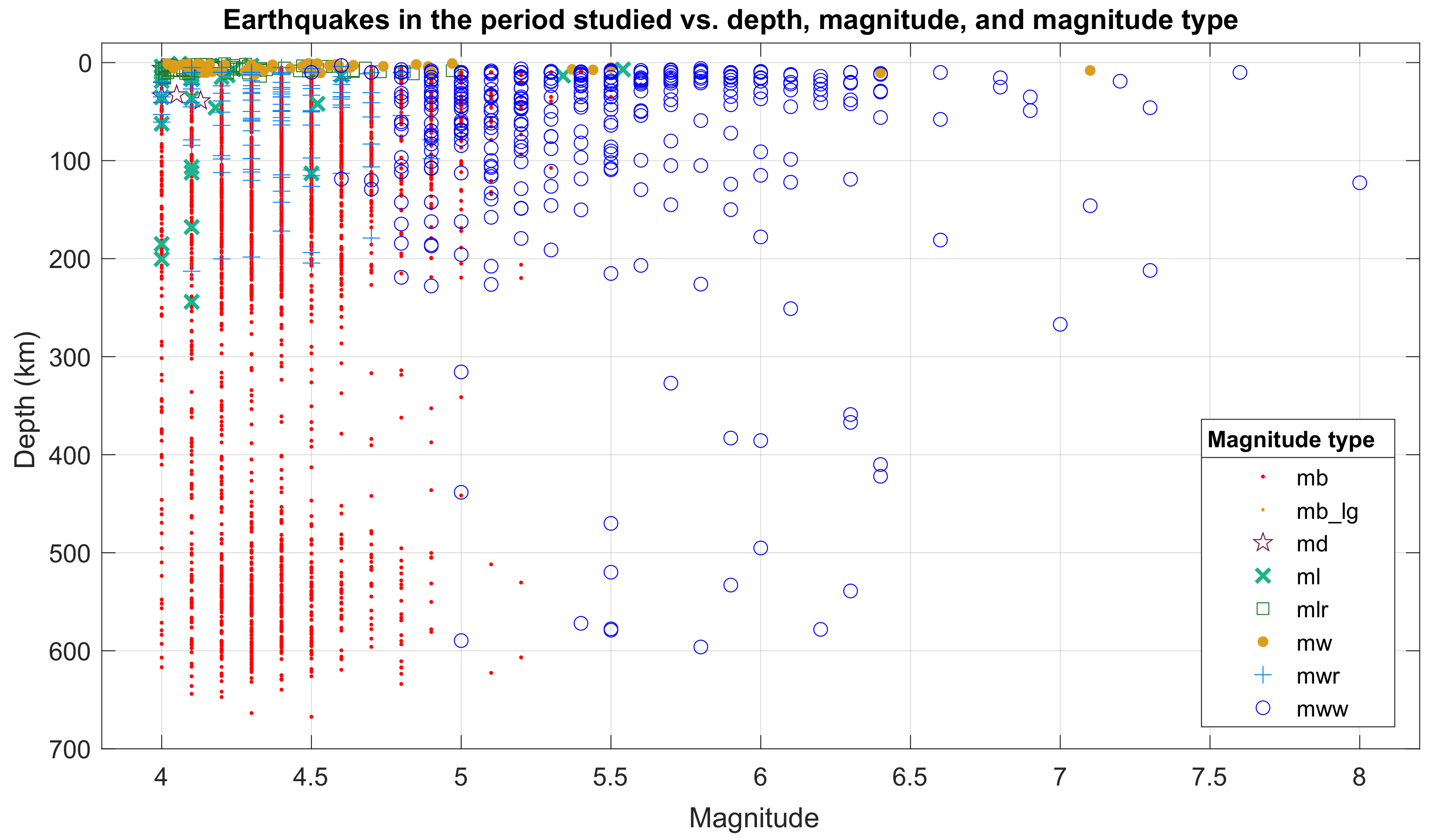
W (usually noted as m_ww) is the one with a wider range of application, extending above M5, and in particular, for large earthquakes (M8 and greater events) is the most accurate one.
In the USGS database, each earthquake in the period studied is given by a single magnitude type [
30], but, as stated before, they are all designed to be consistent. This is why, in our study, the magnitude provided is used for all the earthquakes, without taking into account the magnitude type.
Table 1 shows the relative abundance of each magnitude type in the period studied:
Figure 3 shows the distribution of all earthquakes in the period as a function of their depth and magnitude, and showing the magnitude type with different symbols and colors.
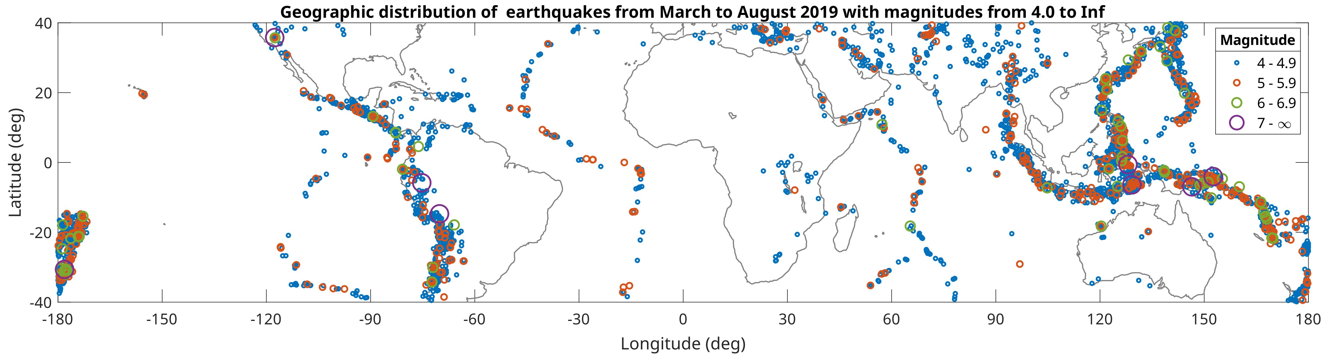
Figure 4 shows the position of all the earthquakes occurring in the six months studied, from March to August 2019. Please note that the color scale and size of the circles represent their magnitudes. It is important to remark that most of them happen in the middle of the oceans, near the faults between tectonic plates. With the method presented here, only these earthquakes in oceanic regions or near the shore can be monitored, because the land reflectivity is highly variable, and the possible ionospheric scintillation would become masked. For example, the largest earthquake in the period studied, with a magnitude of 8.0, on 26 May in Peru, was located on land, 500 km away from the closest seashore, which is larger than the maximum distance considered in this study.
The total number of earthquakes that took place in the period studied is 6108, and 29.4% of them are located on land, but many of them could happen on small islands or very near the shore so they are included.
Figure 5 shows a histogram for all the earthquakes in the period (blue bars), and only the ones happening on land (in brown), as a function of their magnitudes. Please note that the vertical scale is in logarithmic scale to see the larger magnitude intervals, where only a few earthquakes occur.
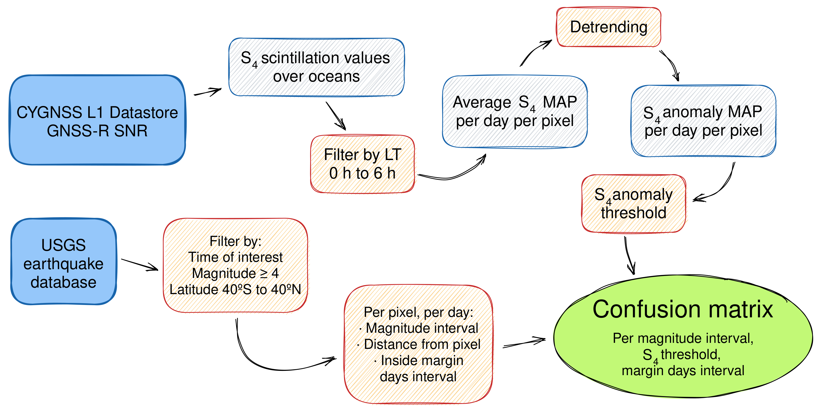
2.4. Confusion Matrix Calculation
Finally, the ionospheric scintillation variation data and the occurrence of earthquakes, are analyzed to assess the correlation of their mutual occurrence, and the confusion matrix is computed. The overall process is shown in the diagram in
Figure 6.
A confusion matrix (CM) is the usual way to study the effectiveness of an algorithm to detect an event. It is a 2 × 2 matrix classifying the events according to two binary classes: the predicted ionospheric scintillation signature, and the actual occurrence of the earthquake. This classification results in four possible cases, as depicted in
Figure 7.
In particular, after the data pre-processing described in previous sections, the creation of the confusion matrix is described below, repeating this classification for each day d and each pixel within the variations map:
The matrix accounts for the total number of events in each of the four categories. As planned, each event studied fit in one, and only one, category. The maximum number of events computed in a CM will be events, where is the number of days under study and is the number of pixels in the map. In our case, using pixels, there are points.
As explained in
Section 2.2, in the S
4 variations maps there could be pixels with no data, either because they are completely located on land, and never fit a specular reflection point or because the LT filter applied removed all the days in the current small window used. This means that the total number of pixels computed (TOT) will be less than the total on the map, in particular, every day, a constant number referring to the land coverage will be subtracted, and then another quantity corresponding to the temporal evolution shown in
Figure 2.
Several confusion matrixes are constructed after setting the different parameters mentioned before, which are detailed in
Table 2:
The parameter is used to study whether there is a preferred time of appearance of the ionospheric anomalies before or after the earthquakes. Please note that when a CM is labeled as , it means that for each day D in which the anomaly is computed, earthquakes are searched within the days days, i.e., the anomalous change in is a precursor of the earthquake. For example, would mean from days.
The parameter is used as a tuning parameter for the binary classification table. A smaller threshold would make the algorithm detect more positives, which includes TP (correct predictions), but also FP (false alarms). The study will be used to optimize this threshold to maximize the effectiveness of the algorithm.
2.5. Statistical Parameters
From the confusion matrix, several metrics were extracted to quantify the goodness of the correlation. First of all, the normalized values of each category in the confusion table are computed according to the expressions in Equation (
3)
The simpler qualifier that can be extracted is the accuracy (ACC), which measures the ratio of correct predictions (TP and TN) among the total cases (TOT) according to Equation (
4):
The F
1 score is the harmonic mean between the
, and the recall or
. F
1 is therefore calculated with Equation (
5):
Another correlation parameter that performs better for unbalanced classifications, in which the number of positives and negatives is very different, is the Matthews Correlation Coefficient (MCC), also called phi-coefficient (
), and it is given by the expression in Equation (
6):
Furthermore, finally, the Diagnostic Odds Ratio (DOR) is a measure of the effectiveness of a diagnostic test, and it is given by Equation (
7). DOR has positive values larger than one when the test is useful and increases as the performance is better.
Additionally, the Receiver Operating Characteristic (ROC) has been calculated. This is a method historically introduced by military radar receivers in the 1950s to diagnose the ability of a system to detect true positives with respect to false alarms. The ROC is the plot of the TPR vs. the FPR when moving a sensitivity parameter. In our case, the parameter is the
, and the curve is studied for the rest of parameters indicated in
Table 2.
3. Results
The results obtained using this technique cover a maximum period of 180 days (6 months) from March to August 2019. To compute the
variations maps as explained in
Section 2.2, it is required to obtain CYGNSS data from at least 60 days before the first day to be studied, so the average
maps were computed from 1 January to 28 August.
Then, the
variations (
) maps were computed for every day between 1 March to 28 August, 180 days in total. As is shown in
Figure 2, there is a temporal variation of the region covered after doing the LT filtering (from 0 h to 6 h) and the seasonal detrending.
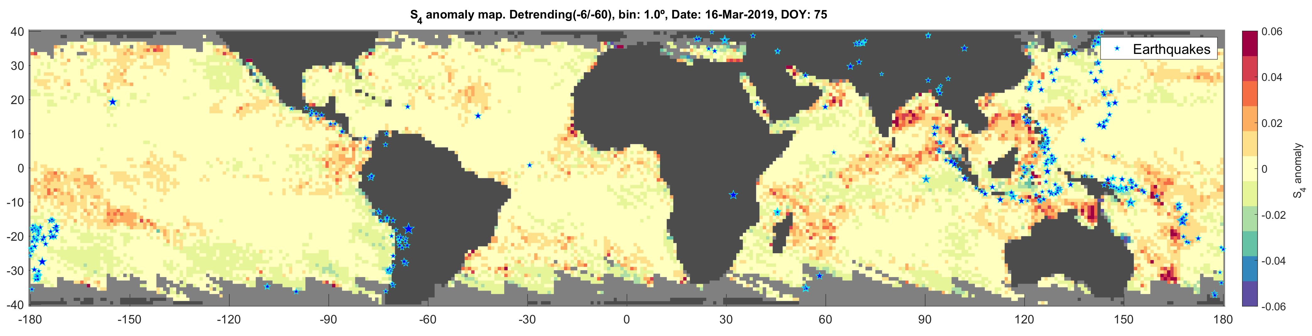
Figure 8 shows this map for one of the days with maximum coverage, almost ranging from −40º to +40º.
The image shows the results of the detrended values for the selected day over oceanic regions with the values ranging from −0.06 to 0.06 as indicated in the color scale. Blue stars mark the epicenter of all earthquakes happening during the period from −6 days to +6 days from the current day 16 March.
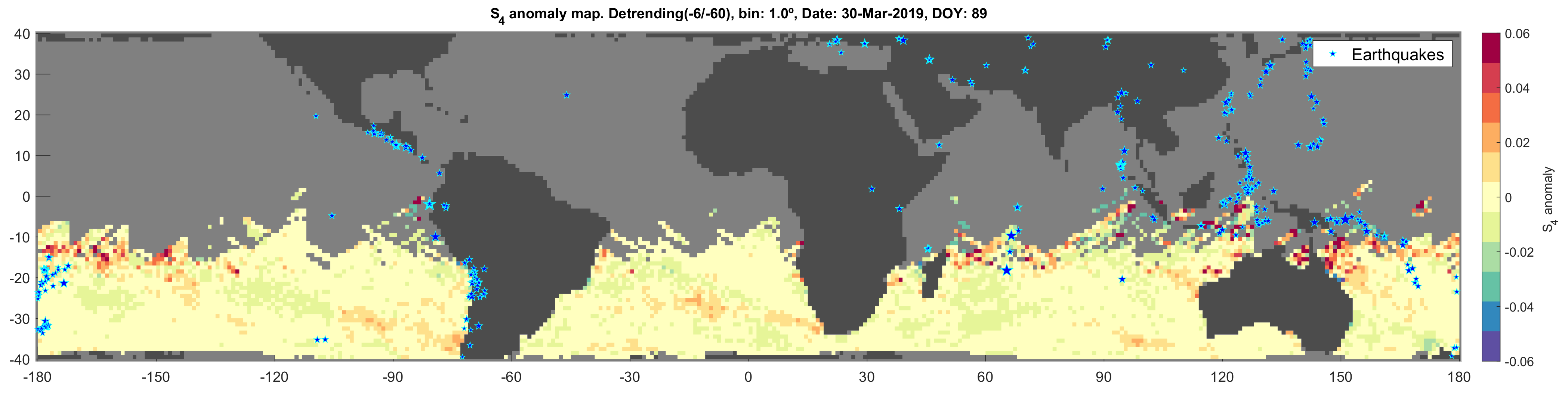
Figure 9 shows the
variations map for a day in which the coverage is minimum, 30 March, in this case corresponding to the southern part. It can be observed that still several regions can be used to correlate ionospheric scintillation anomalous variations with earthquakes.
3.1. Case Studies
Before a more quantitative, global statistical analysis is made, some case studies are presented to visually check the results of the technique proposed. To do that, videos were created showing the daily
overlapped with the earthquakes. These videos are provided as
Supplementary Materials.
Video S1: anomaly_s4_180days_fullCoverage.m4v shows the full region covered by CYGNSS for the whole period covered in the study, and
Video S2: case_study.m4v show the period and region corresponding to the case study detailed here. As in the previous figures, in the videos, earthquakes are kept in each frame for six days before they occur until six days after, so it is possible to visually check whether there is an increasing
anomalous deviation before the occurrence of an earthquake, and if it stays for some time after the earthquake happens.
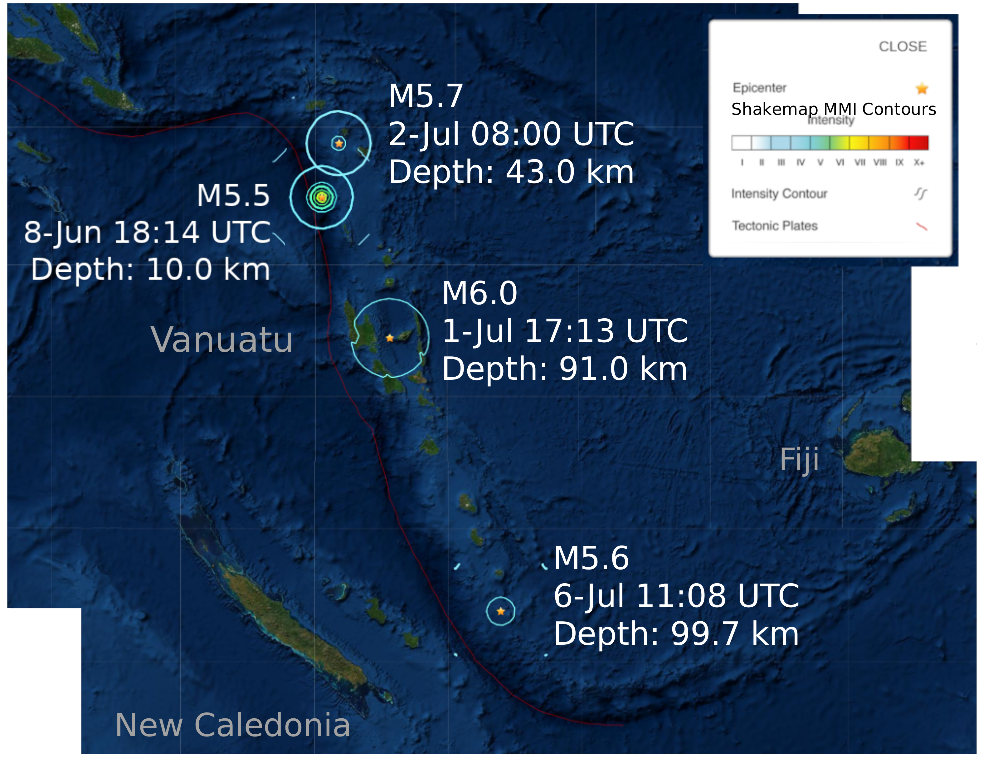
A case in which some positive variations in the
index are distributed around an earthquake cluster occurred at the beginning of July 2019, in the oceanic region of Vanuatu’s archipelago. Vanuatu is a group of islands of volcanic origin that formed after the subduction of the Australian plate under the Pacific plate, which makes this region suffer from large recursive earthquakes [
32]. Some of the largest earthquakes from the cluster mentioned are shown in
Figure 10, indicating their magnitudes, UTC times, and depths. Please note that all of them are located eastward of the fault, where the subduction takes place. The circular curves around the earthquakes indicate the shakemap Modified Mercalli Intensity (MMI) contours, which are defined from I to X measuring the intensity of the effects produced on the surface.
During the last few days of June and the first week of July, several positive variations in the ionospheric scintillation values were found in this region. Moreover, the anomalies appear after a period of stabilization in the scintillation activity, indicated by close-to-zero values in most of the area.
Figure 11a shows the map of the region around the Vanuatu archipelago for 30 June, a few days before the earthquakes shown in the previous image.
Figure 11b, shows the map for 1 July, the day of the strongest earthquake (M6.0) in this cluster, and an increase is observed in the closest pixels to this earthquake, and also in the Southern New Caledonia region.
Figure 11c corresponds to 4 July, and the peaks in
variations are now clear in the whole area, and that can also be related to other earthquakes happening in 6 July in the South. It is important to remark that
is computed from the average of the previous 7 days, so, variations are shown for the same day
D are produced before it, even if the day
D is a few days after a particular earthquake.
Finally,
Figure 11d shows 7 July, in which the positive values in the
deviations persist although the northern region is starting to miss data due to the oscillation in the region covered shown before.
3.2. Temporal Analysis around Earthquakes
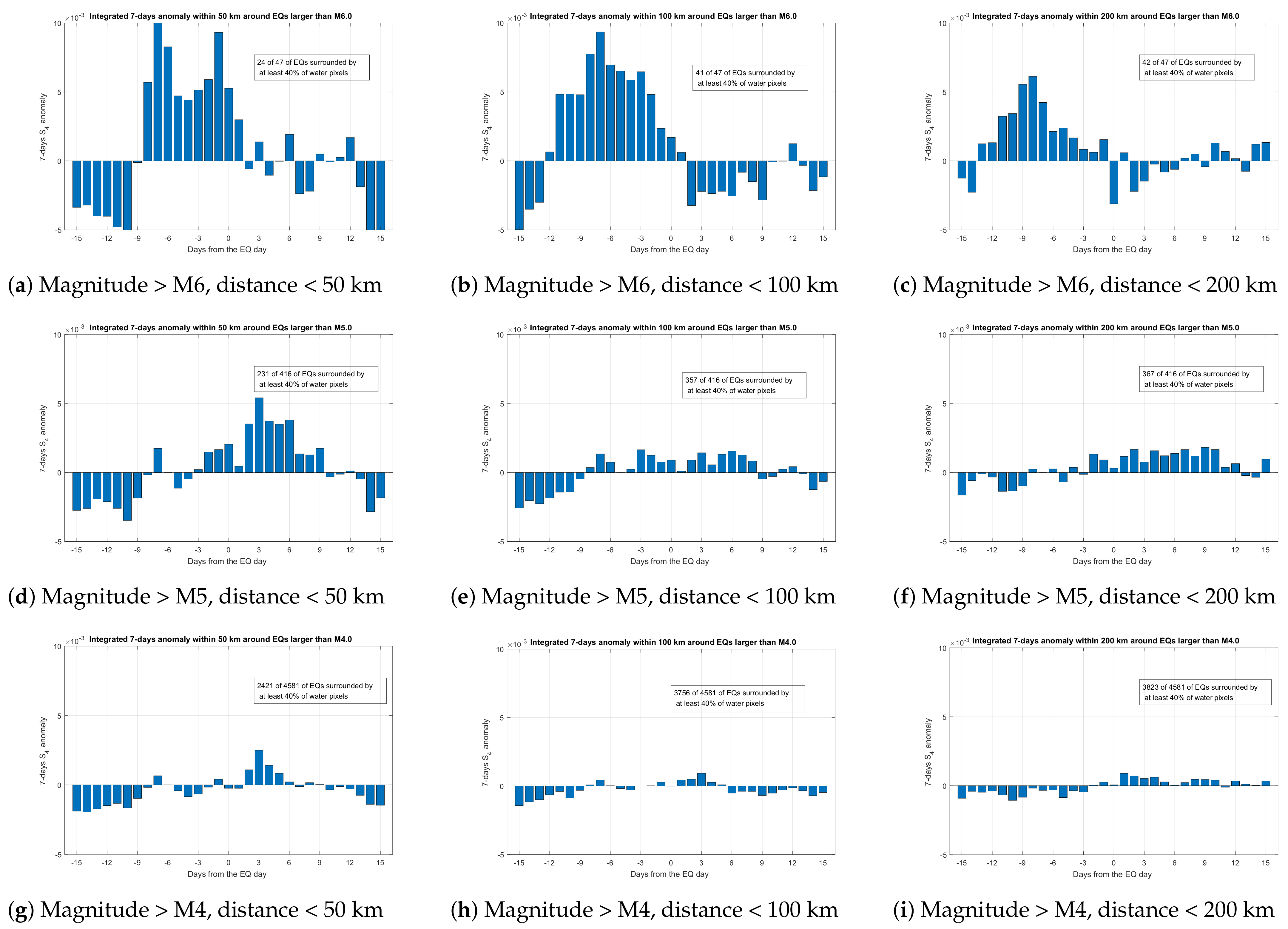
In this section, the results of a more detailed temporal analysis of the changes are presented. The purpose is to study the temporal evolution of the changes around the earthquakes in the period under study. The way to measure this evolution is by averaging all the pixels in the deviations maps that fall inside a circle of a given radius around each earthquake and computing this average for each day during a period of some days before and after the earthquake day.
Figure 12 presents different plots for different minimum earthquake magnitudes in rows, and different integration radii, in columns. Each plot shows the averaged
value of all the pixels inside a circle centered in the earthquake epicenter from 15 days before to 15 days after the event, and then averaged for all the earthquakes in the period from 1 March, to 29 August 2019. Only earthquakes that are surrounded by at least 40% water pixels are computed in this average. This filter is applied to remove false alarms due to earthquakes that occur on land, but close enough to the sea to have enough pixels with valid data. A low number of data points to average may produce unrealistic results. The total number of earthquakes in this period, and those remaining after filtering with the water coverage, are shown in each graph.
The results in
Figure 12 are divided in rows according to the earthquake magnitude lower limit. For the largest magnitude interval, M6 and larger (
Figure 12a–c), it is observed that for the 10 days before earthquakes, the value of seven days
is positive and larger in magnitude than the rest of the days, particularly, the ones after the earthquakes. Similar behavior is observed using different integration radii (50 km, 100 km, 200 km), only showing a small decrease in the peak when integrating larger radii. This is the expected response, as the larger the area to estimate scintillation, the more uncorrelated noise in the circle.
In the next figures for smaller magnitude intervals (from M5 and M4), a decrease in the peak amplitude is observed, which reduces with decreasing earthquakes’ magnitude and larger radii. Furthermore, please note that the position of the peak has moved towards the right, indicating that the scintillation positive anomalous increments occur now closer to the event of earthquake. Since the seven day window introduces a 3.5 day, a positive
peak at
means that the precursor occurs just the day before the earthquake (
Figure 12d).
3.3. Confusion Matrix Analysis
The qualitative results shown in the previous case studies are only some particular cases to illustrate the technique. A more robust and quantitative way to study if this technique is effective in detecting earthquake-related ionospheric anomalies is to perform a correlation test of the data by means of the confusion matrixes introduced in
Section 2.4.
As explained, the variations maps from the full period of 180 days are computed pixel by pixel classifying them in the four categories depending on whether they are positive or negative cases for both the value and the earthquake occurrence. With these results, it is possible to construct the confusion matrix, and its derived statistics for each set of parameters.
Table 3 shows a subset of the total number of CMs computed. All of them are calculated for 180 days of data using:
Remember that the total number of events computed, marked as TOT is the total number of pixels with valid data during the period studied. Positives (P) and Negatives (N) refer to the pixels with earthquakes closer than the radius, and TP, TN, FP, and FN are the four categories of the CM.
The results of the statistical parameters described in
Section 2.5 are presented here in
Table 4 for each case studied, for the same previous cases used in
Table 3.
As introduced in
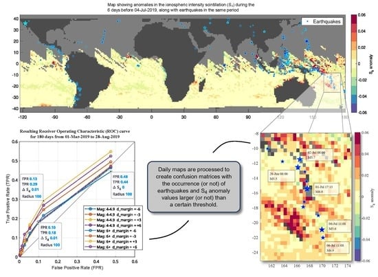
Section 2.4, the Receiver Operating Characteristic (ROC) curves are also a good way to identify better performance of a classification algorithm and to tune the threshold parameter used, in this case
. The ROC curve is constructed by plotting the TPR vs. the FPR, so it is able to compare simultaneously the performance of the algorithm to correctly associate positive changes in the
value with earthquakes against the rate of false alarms produced when the algorithm detects an positive change in the scintillation, but there is no earthquake in this region and period.
ROC curves for the three magnitude intervals are presented in each of the plots in
Figure 13. Four curves per graph are shown with different colors indicating the time interval from the anomaly to the occurrence of the earthquakes, being positive when it is prior to the earthquake so it could be considered as a precursor.
Each point in the curve is for a different value of the threshold parameter
shown as rows in previous
Table 3. Please note that the point closer to
is the one the with largest
, which makes sense because larger threshold are filtering more true detections, and also reducing the false alarm rate. Decreasing the threshold in 0.003 intervals, both parameters increases until the last point (the one closest to
) for
.
ROC curves indicate better performance when they are more separated from the line, which would be the result of a completely random detection algorithm. ROC-AUC (ROC Area Under the Curve), is a good indicator of this performance, and it will be discussed in the next section.
Figure 14 and
Figure 15 show the ROC curves for the three magnitude intervals using a radius of 50 km and 100 km, respectively. In these plots,
has been swept from 0 to 0.04 in intervals of 0.01.
4. Discussion
The results presented here are showing a small, but positive correlation between the occurrence of earthquakes and the anomalous variations of ionospheric scintillation. The confusion matrix shows the values for the True Positives, True Negatives, False Negatives, and False Positives integrated for all the days in the period studied. The positives (P) show the number of pixels with at least one earthquake within the radius distance, and it is only varying when this parameter changes. For example, in
Table 3, is 363 for all cases, as the radius is always 100 km.
It is observed that when the threshold () increases, the number of true positives (TP) and false positives (FP) both decrease. The relative ratio of change is studied with the ROC curves. Larger values of the TPR with respect to the FPR for the same threshold mean that is more probable that a positive in the predicted condition (ionospheric anomaly) is associated with an earthquake event, than it is not, and they will be represented by curves above the diagonal.
Figure 13 shows the ROC for the three magnitude intervals. All of them show a small, but positive indicator, with curves above the main diagonal for almost all the threshold values selected. What is also very interesting is that, as the magnitude of the earthquakes increases, the curves are further from the diagonal, and also they separate from each other. In the last graph (
Figure 13c), for magnitudes larger than 6, curves for
and
are above their corresponding negatives values. This means that for the largest earthquakes a better correlation is observed when the anomalies are recorded a few days (3 to 6) before the earthquakes.
Similar results show the ROC curves in
Figure 14 and
Figure 15, which have been drawn using a coarser
interval. In this case, for the 50 km radius and magnitudes larger than 6 (
Figure 14c), we observe that only the one corresponding to the
is separating from the main diagonal. Here we can see that the correlation is less when the radius decreases from 100 km to 50 km.
The values of the ROC-AUC are also a good indicator of the performance of the correlation. Please note that in all the ROC curves shown before in
Figure 13, none of their values reach the point (1,1) even that the sensitivity parameter,
, has been swept from 0 to 0.03 or 0.04.
is the one closer to the (1,1), but decreasing this value under 0 makes no sense as it would mean considering a detection when the average
during the last 7 days has been larger than a value lower than the last 2-month average. Then, the ROC-AUC has been computed using the data points shown in the curves, and adding the points (0,0) and (1,1), doing a linear extrapolation. The resulting areas are shown in
Table 5 and
Table 6.
Table 5 for
identifies the magnitude larger than 6, as the set of curves with larger ROC-AUC values in general, being the largest one, 0.5766, when the interval for
is
, closely followed by the
. The rest of the table exhibits values around 0.52, very similar among them, remarking the similarity among the curves for the lowest two magnitude intervals in
Figure 13.
Table 6 shows the results of the ROC-AUC for
. In the case of the largest magnitude interval (above 6), as observed in
Figure 14 the ROC lines are closer to the main diagonal, or even under it, resulting in ROC-AUC values under 0.5. In this case, the better results in terms of ROC-AUC values are for the lower magnitude intervals, [5–5.9] and [4–4.9]. This may be an indicator that smaller earthquakes may produce perturbations at smaller distances from the epicenter.
Another way to analyze the correlation between both events is through the statistics extracted from the CM. In particular, the values of the DOR are shown in
Figure 16. The DOR, given by Equation (
7), is an indicator of the diagnostic performance that takes into account the whole parameters in the CM and it ranges from 0 to infinity, being larger than one for positive correlations, and higher for better performance. In the plots, it is shown that it goes from 1 to 3 or 4 (depending on the case) as
increases.
Figure 16a, for the magnitudes from 4 to 4.9 we can see that all the curves for different
values are very similar, and they separarte for the largest magnitude intervals, as in
Figure 16c, where the largest DOR is almost 5 for a
and
.
Another metrics computed is the accuracy (ACC) using Equation (
4), which is shown in
Figure 17 for the 100 km radius case. The problem with this indicator for very unbalanced classifications such as this is that they will give unrealistically high values because they are only accounting for the TP and TN counts with respect to the total TOT. It is observed in the plot that it goes from 50% accuracy to almost 100%, and all the curves are overlapping in the one shown here, for all
, and all magnitude intervals. In this case, as the number of Positives (P) and Negatives (N), i.e., earthquakes vs. no-earthquakes, is very unbalanced, the accuracy is not a good indicator of correlation.
To complete the analysis, curves for the F
1 score and Matthews Correlation Coefficient (MCC) are shown in
Figure 18 and
Figure 19, respectively. F
1 score is an improvement of the ACC parameter, but still, it is less indicative than the DOR or the MCC for this case. Remember from Equation (
5), that the numerator is only accounting for the true positive (TP) cases, which for this study are decreasing a lot for large magnitudes intervals, which explains the low values in the plot in
Figure 18c.
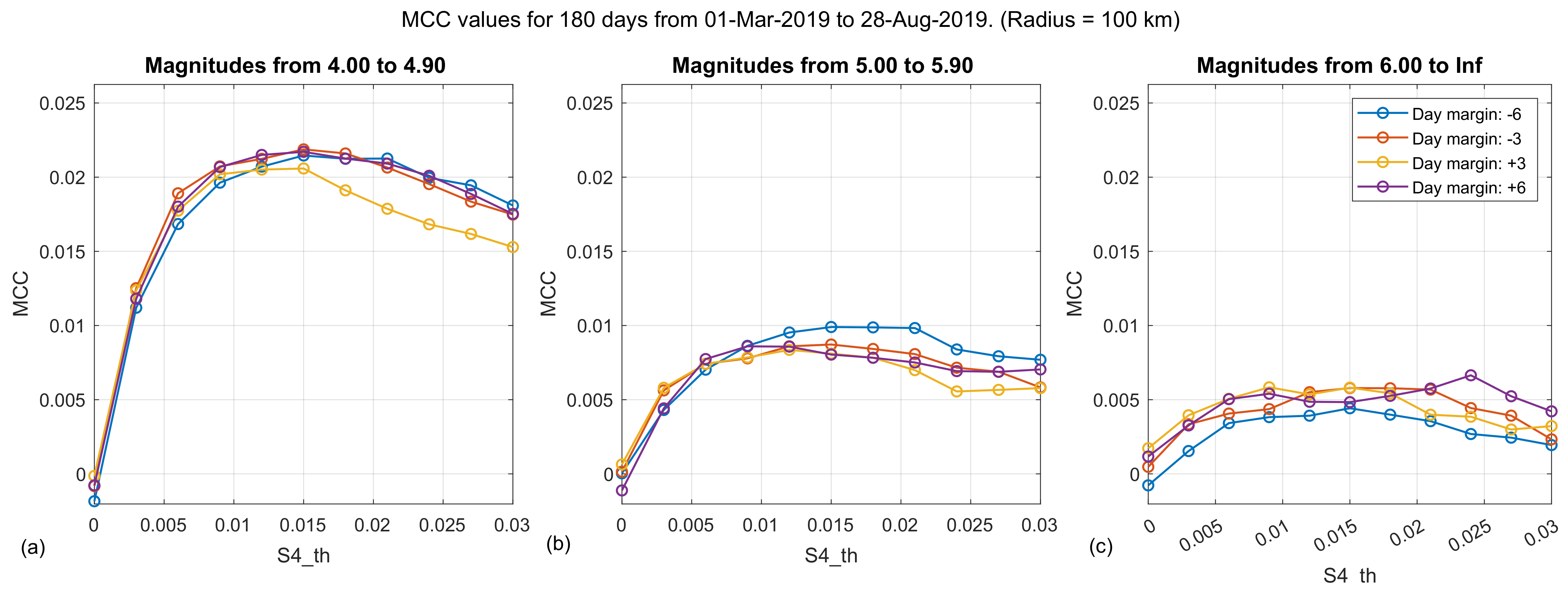
Finally, the MCC is shown in
Figure 19a–c and it indicates positive values for all magnitude intervals. MCC ranges from −1 to +1, being zero when there is no correlation. In the same way as other parameters studied here, MCC is indicating positive values although they are small. As the F
1 score, the MCC shows smaller values for the largest earthquake magnitudes, the height of the peak is decreasing from
Figure 19a to
Figure 19c.
An interesting conclusion that can be extracted from the two most significative statistical parameters (DOR and MCC), is the value of the ionospheric scintillation threshold (
) parameter that is giving the best performance when correlating earthquakes with
positive variations. As observed in
Figure 16a,b for small magnitude intervals (from 4 to 6), using the DOR metrics,
is larger than 0.03 (the largest value swept), but it is close to 0.02 for magnitudes larger than 6, in
Figure 16c. For example, the values previously shown in
Table 4 correspond to the yellow line (
: +3 d) in
Figure 16c, which has a peak
for a
.
In the case of the MCC it also exhibits a peak in the interval studied, which falls around 0.01–0.015 for lower magnitude intervals, from 4 to 6, and it is a bit wider for large earthquakes, ranging from around 0.006 to 0.020.
The position of both peaks in DOR and MCC also matches the values of
in which the ROC curves are further away from the main diagonal, as found in
Figure 13,
Figure 14 and
Figure 15.
5. Conclusions
This study used six months of data from the NASA CYGNSS GNSS-R mission from March to August 2019 to estimate ionospheric amplitude scintillation to try to analyze possible correlations between the occurrence of earthquakes and the associated changes in the ionospheric amplitude scintillation index , and also try to determine if these changes are produced with higher probabilities before (as a precursor) or after the earthquakes. The technique used computes the confusion matrix (CM), a usual technique in diagnostic tests, e.g., in medical sciences or machine learning algorithms, to quantify the goodness of a diagnostic test.
The results presented in this work show a small, but detectable, positive correlation for all earthquakes with magnitudes above 4, with better results as the magnitude increases. A slightly better correlation was also observed when the positive increments in the index are observed between 6 and 3 days before the earthquakes, with respect to the ones observed after them. These results have been extracted from the analysis of ROC curves for different magnitude intervals showing the relation between the probability of finding a correct prediction vs. a false alarm. In the best cases, the correct prediction probability is around 32% and the false alarm probability is 16%.
It should be also pointed out, that the probability of detection is small for all the cases. In our opinion, despite these results showing possible evidence of ionospheric scintillation increments as precursors of earthquakes, mostly for the largest magnitude ones, the signature is still small, and it should not be regarded as an early warning system for earthquakes. Moreover, the study was made using earthquakes during a 6 month period, when only a small number of large earthquakes () took place, specifically 68. From them, only 47 were in oceanic regions. Moreover, the region covered by CYGNSS is always close to the geomagnetic equator, where ionospheric scintillation is also more probable to appear.
The novelty of this study lies in the use of GNSS-R global oceanic data to measure amplitude scintillation positive increments as a possible precursor for earthquakes. Other studies detected anomalies in the ionosphere, but they were mostly related to changes in the Total Electron Content (TEC) after the earthquakes, which can be produced by the mechanical energy transmission from the sudden crust movement through the atmosphere to the ionosphere. Furthermore, few of the previous studies used satellite data, allowing the possibility to perform global studies such as this one, and they were focused on particular cases using local GNSS ground stations.
Future work will extend this study using longer periods of time, and larger Earth coverage. CYGNSS constellation used to obtain the GNSS-R data used here only covers from 40ºN to 40ºS, which is good to have a better revisit time, but it is missing earthquakes occurring at higher latitudes. Furthermore, this technique, using GNSS-R is only valid for calm oceanic regions, which loses around 30% of the earthquakes. So, a possible way to study ionospheric scintillation on land would be to use GNSS Radio-Occultation (GNSS-RO) data as well. Using this technique the overall performance may be even better as it does not suffer from the ocean surface conditions.


