Threat Matrix: A Fast Algorithm for Human–Machine Chinese Ludo Gaming

Abstract

Chinese Ludo, also known as Aeroplan Chess, has been a very popular board game for several decades. However, there is no mature algorithm existing for human–machine gambling. The major challenge is the high randomness of the dice rolls, where the algorithm must ensure that the machine is smarter than a human in order to guarantee that the owner of the game machines makes a profit. This paper presents a fast Chinese Ludo algorithm (named “Threat Matrix”) that we have recently developed. Unlike from most chess programs, which rely on high performance computing machines, the evaluation function in our program is only a linear sum of four factors. For fast and low-cost computation, we innovatively construct the concept of the threat matrix, by which we can easily obtain the threat between any two dice on any two positions. The threat matrix approach greatly reduces the required amount of calculations, enabling the program to run on a 32-bit 80 × 86 SCM with a 100 MHz CPU while supporting a recursive algorithms to search plies. Statistics compiled from matches against human game players show that our threat matrix has an average win rate of 92% with no time limit, 95% with a time limit of 10 s, and 98% with a time limit of 5 s. Furthermore, the threat matrix can reduce the computation cost by nearly 90% compared to real-time computing; memory consumption drops and is stable, which increases the evaluation speed by 58% compared to real-time computing.

1. Introduction

Board games are a form of intellectual confrontation invented over the course of a long history of production activities [1,2]; in addition, they are important applications that can help to explore and promote research into artificial intelligence [3]. The selection of pieces depends on a perfect evaluation function with a computation complexity of approximately $b^d$, where b is the number of legal moves per position and d is the number of positions of the chessboard. Because different types of board games have different b and d, the total amount of calculations varies greatly [4,5]. The evaluation algorithms of chess programs involve various artificial intelligence (AI) techniques, including machine learning, expert systems, neural networks, search trees, etc. [6,7]. The critical jobs that most game software focuses on consist of two aspects: (1) how to define and obtain comprehensive evaluation factors; and (2) how to construct a perfect evaluation function.

The advance of AI chess can be attributed to two factors: (1) high performance computing devices [8]; and (2) powerful evaluation algorithms [9]. In recent years, with the rapid development of high-performance computing and network technologies, as long as a suitable evaluation algorithm can be constructed a computer will be able process a very large number of calculations. With the recent rapid development of high-performance computer and network technologies, as long as the evaluating algorithm is properly constructed the huge amount of computation can be handled by machines [10,11]. Because machines are accurate, fast, and not influenced by emotion, they often beat human players. At present, computer players of classic board games such as chess, Go, Shogi [4], and Checkers [12] can beat expert human players. R. Ruben et al. [13] have described a general video game AI (GVGAI) that provides a way to benchmark AI algorithms for games written in specific description languages for many application domains. The continuous promotion of AI algorithms from games to reality is of great significance for the development of both robot swarm intelligent collaboration and gaming [14,15].

The world chess champion Garry Kasparov was defeated by IBM’s Deep Blue computer, which has become a milestone in the advance of artificial intelligence over human beings. Deep Blue typically searches to a depth of between six and eight moves up to a maximum of twenty moves, or even more in certain positions [16]. This brute force type of search can benefit to a degree from advances in computer performance. However, moving from brute force to informed search is a great endeavour in AI board game research. A recent study by Ansk involved an idea to solve two-player zero-sum and extensive-form games [17]. They were able obtain perfect information and simultaneous moves using the Double-Oracle Method and Serialized Alpha-Beta Search. In addition, Branislav et al. [18] are devoted to developing synchronous move game algorithms and evaluating exact backward induction methods with efficient pruning and sampling algorithms under different settings. David B. and his group focus on evolutionary algorithms, while Sebastian presents a rules learning method for general game playing. Thus, this great endeavour requires a combination of methods from a variety of subdisciplines [19,20].

Due to the enormous search space needed for the combination of large moves, the development of a program that can beat humans at the ancient Chinese chess-like game Go has been considered as one of the last great challenges [21,22]. Tesauro’s approach is already considered to outperforms the best human players in playing backgammon. AlphaGo [3], developed by Google DeepMind, has beaten a top professional human Go player without handicaps on a full-sized 1919 board. AlphaGo’s algorithm uses a combination of machine learning and search tree techniques combined with extensive training on both human and computer play [23].

Similar to chess, Go, and backgammon, Chinese Ludo gaming, known as Aeroplan Chess, was invented in China by reference to other ancient board games to commemorate the Flying Tigers in World War II; the game’s rules and paths are derived from Lufbery circles in air warfare [24]. To encourage students to master chemical equations in the game, a new flying chess game called CHEMTrans has been developed.

In recent years, many online programs for Chinese Ludo gaming have been developed. These simply provide a platform for interaction between game players, and the computer does not engage in intelligent competition [25]. Developing a human–machine Chinese Ludo gambling game, while an attractive idea, represents a highly challenging task. Apart from the high randomness of the dice rolling, the algorithm must ensure that the machine is smarter than humans in order to guarantee that the owner of the game machines makes a profit. As a game requires 2–4 players and random dice rolling, no such gaming machine has been developed [26,27].

It is an interesting idea and a challenging task to adapt Chinese Ludo to the gambling industry. Despite the randomness of the game, the game machines must be “smarter” than people to ensure that the game owners make money. The primary contributions in this paper are as follows.

• We develop a human–machine gambling Chinese ludo game which is unlike most other chessboard programs; while these involve brute-force algorithms that require high-performance machines, our evaluation function is a simple linear sum of four variables.
• For high-frequency threat computation between any two dice, we innovatively propose the concept of a ‘threat matrix’. Using the threat matrix, our program can instantly acquire the threat value between any two positions, rather than relying on brute-force computing based on the current positions. As a result, our program can reduce the real-time (immediate) computation cost by nearly 88%.
• Threat matrix can run on an 80 × 86 SCM (Single-Chip Microcomputer), and has achieved a 97% winning rate against human players.

The rest of this paper is organized as follows. Section 2 briefly introduces the rules of the Chinese Ludo game and reviews related existing research works. Section 3 provides details on the evaluation function, threat matrix, and our proposed algorithms. To clearly show how to calculate the evaluation function, Section 4 presents a concrete example. Section 5 analyses and compares the complexity of the main algorithms. Section 6 presents experimental validations and shows comparisons of various strategies. Section 7 concludes the paper.

2. Chinese Ludo Game

In this section, for convenience in understanding our algorithms we first briefly introduce the rules of improved man–machine gambling Chinese Ludo by the Lanhai Technology Company. Note that while the rules may be slightly different among different versions, the main rules are always the same.

• Composition

  (a)

  Dice: One traditional dice, with each of its six faces showing a different number of dots from 1 to 6.

  (b)

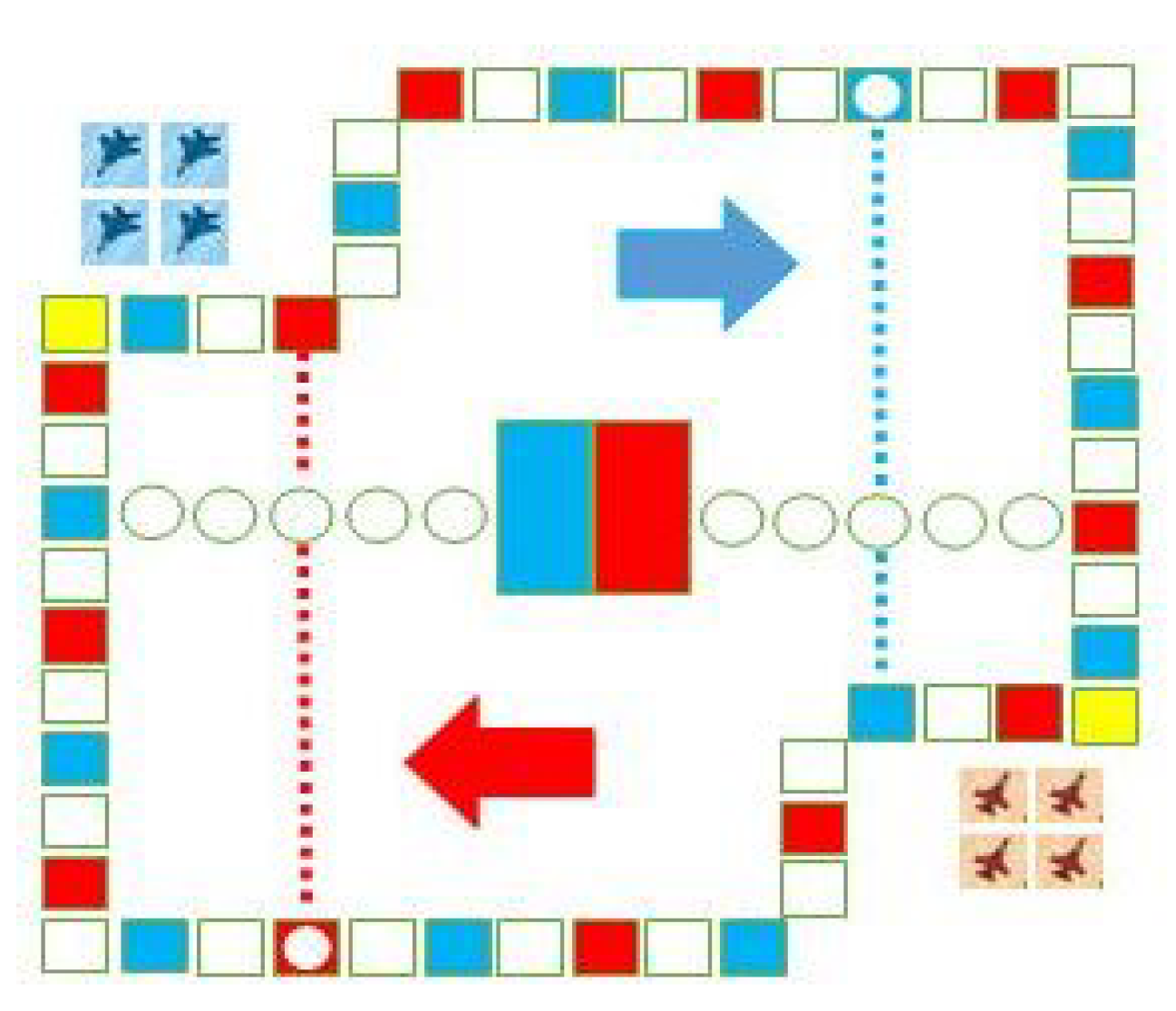
  Board: One board, as shown in Figure 1, with 64 square positions marked with different colors. Each player is assigned a color, either red or blue. The top left corner and the right bottom corner are staging areas (‘hangars’) and the two closed rectangles colored with red and blue in the center are the ending squares corresponding to each game player.

  (c)

  Planes: Each player has four planes, in colors matching those of the board. There are two players, one human and one machine, and eight planes in total.

2.

Game rules

(a)

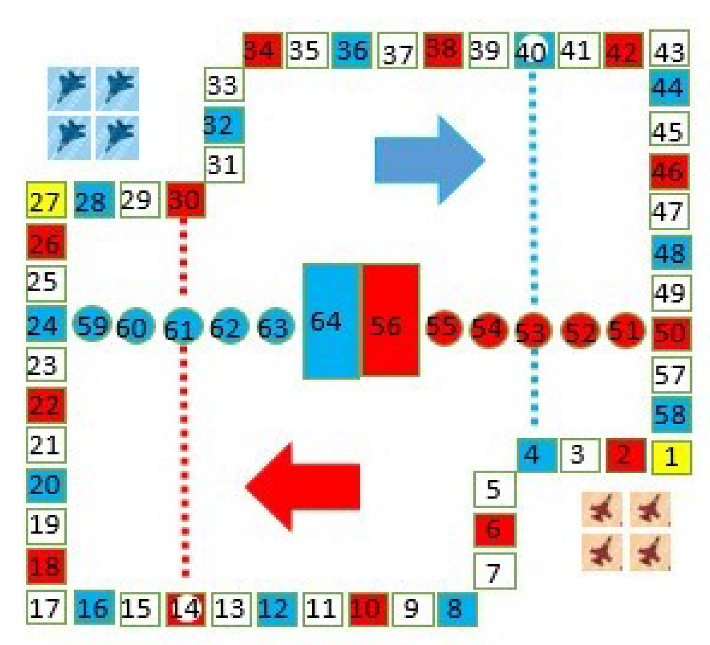
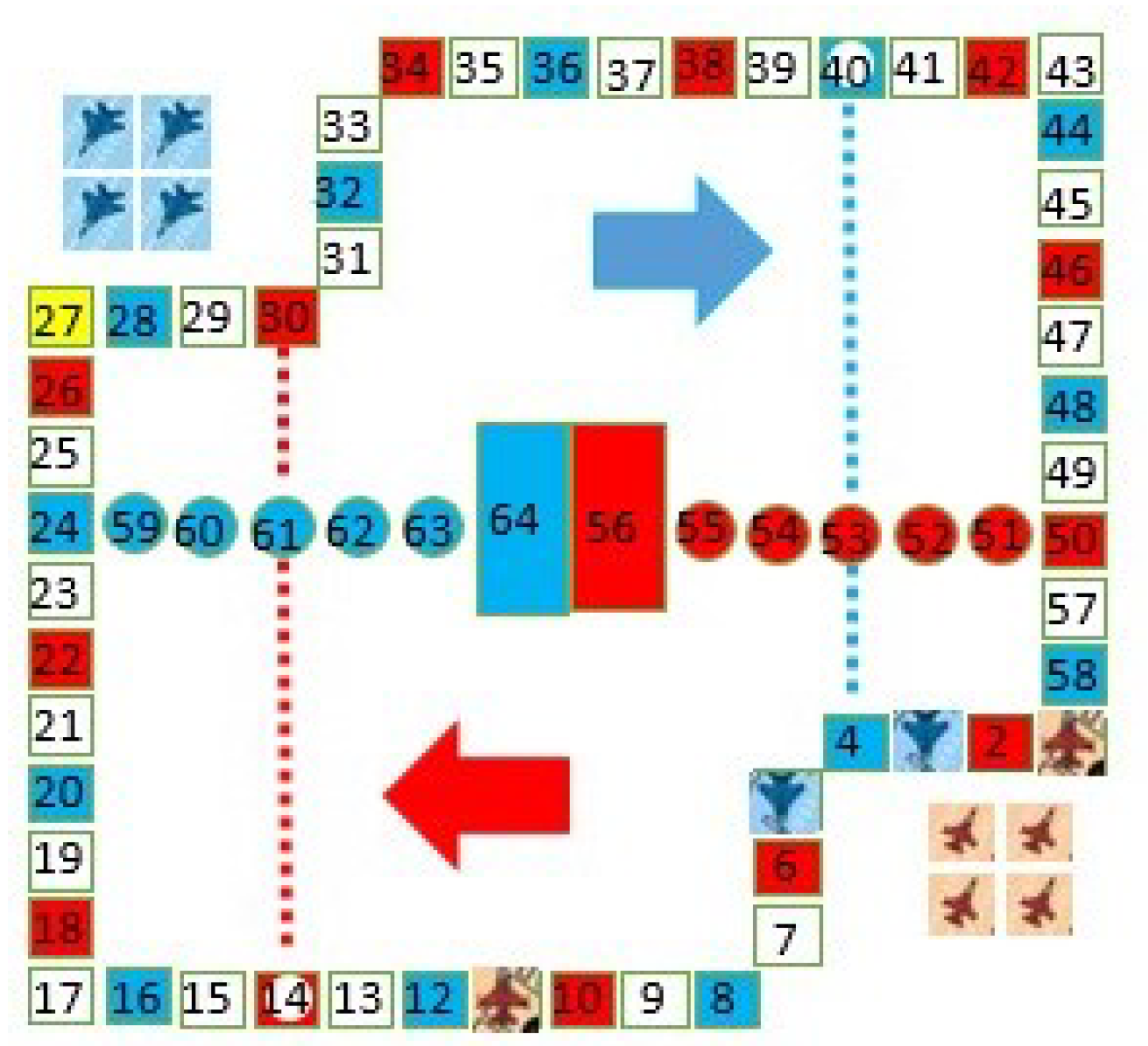
Launch: At the start of the game, all of the planes of the two players are in the staging area. After randomly determine a player to roll the dice first, the players take turns rolling the dice. Only when a player rolls a 6 can s/he select one of her/his planes from its staging area to prepare to fly (in its starting square); the planes fly in the clockwise direction.

(b)

Move: When a player has one or more planes in play, s/he selects one to move (fly) over squares of the number shown on the dice. If the landing square is the same color as the plane’s color, the plane can fly directly to the next square in the same color; however, this cannot be done with circles, which is called a ‘jump’. Furthermore, if the landing square has the same color and is connected with a dotted line, the plane can fly along the dotted line, which is called a ‘dotfly’. The rolling of a 6 earns the player an additional roll in that turn, which can repeat until the roll is not 6.

(c)

Hit: If the landing square is occupied by the opponent’s plane(s), the opponent’s plane(s), either one or more, is hit and forced to return to the staging area. Planes of the same color are not hit.

(d)

Win: The first player who is able to fly all of her/his planes to the ending square wins the game.

3. Evaluation Function

According to the rules of the Chinese Ludo game, the number that the dice shows after rolling is random, and the player has to decide which of her/his planes at different positions to select. Thus, in addition to luck, for a given position winning or losing depends on the selection of planes.

Compared to traditional chess games, the randomness of the dice in Chinese Ludo brings uncertainty to the evaluation of potential moves. Additionally, multi-layered nesting judgement resulting from the rules can introduce looping and crashing during the game. These two key difficulties may explain why there is no mature algorithm for Chinese Ludo gaming suitable for human–machine gaming.

Without loss of generality, let us suppose the computer is blue and the opponent is red. In the rest of the paper, we use blue for computers and red for their human opponents.

3.1. The Description and Definition of the Chess Position

To facilitate the evaluation of the planes, we first define the chess position. First, the squares in the chessboard are numbered as shown in Figure 2. For planes of the same player, the only difference is their position (i.e., different squares). Thus, we can use the number to represent each plane’s position on the game board. The position of each of the four blue planes is denoted by $X_i$ with $(i=1,2,3,4)$. Similarly, the position of each of the red planes is denoted by $Y_j$ with $(j=1,2,3,4)$. We use $S(X_1,X_2,X_3,X_4,Y_1,Y_2,Y_3,Y_4)$ to represent the eight planes’ positions on the board and R to represent the number that the dice shows after rolling. Thus, $(S,R)$ can determine a specific Chinese Ludo position.

3.2. Evaluation Function

Next, we define the value of a position, denoted as $I\left(X_i\right)$, which is the number of squares from the starting square to the current position; $I\left(X_i\right)$ varies with the change of $X_i$, and the closer it is to the ending square, the greater it is. Note that the position of blue restarts from 1 after a modulo operation of 26.

At a chess position $(S,R)$ we need to define an evaluation function, f, in order to determine which plane to move. Obviously, f is determined by position $(S,R)$; thus, we use $f_i(S,R)(i=1,2,3,4)$ to represent the evaluation function of the i-th blue plane at position $(S,R)$. By computing and comparing $f_i(i=1,2,3,4)$, we can make our decision as to which plane to move. Certainly, $f_i(S,R)$ can be used to evaluate the red/opponent’s planes as well.

Considering the game rules, we analyze the four key factors that affect $f_i(S,R)$, as follows.

First, according to its rules (see Section 2), Chinese Ludo allows Jump and Dotfly moves. Therefore, planes at different squares may move different distances with the same dice roll. This is referred to as ‘Incremented Distance’, denoted by $V_1$. Without considering other factors, players intend to choose the plane that can move the longest distance.

Second, we consider Hits, i.e., whether, after moving, a blue plane lands on a square occupied by a red plane and the red plane is hit back to its staging area. We call this the ‘Opponent’s Hit Value’, denoted by $V_2$. Clearly, $V_2$ greatly reduces the chances of the opponent/red player winning and increases the chance that the blue player wins.

Third, if after moving a plane does not hit the opponent’s plane on the current roll, it may hit the opponent’s plane on the next roll. This means that a plane’s threat to the opponent’s planes changes with each move. Certainly, players intend to choose the plane which offers the largest increase in the threat, which we call the ‘Increased Threat Value of Blue on Red’, denoted by $T_1$.

In the same way, the threat represented by the opponent’s plane changes after each move. We aim to choosing the plane which will result in the smallest increase in the opponent’s threat, which we call the ‘Increased Threat Value of Red on Blue’, denoted by $T_2$.

Through the analysis of the above four factors, it can be seen that all four values actually reflect changes in position, and position is the ultimate determination of which player wins or loses the game. Thus, the four values are linearly correlated with the evaluation function, $f_i(S,R)(i=1,2,3,4)$, where the evaluation function is defined as

$$f_i(S,R)=V_1+V_2+T_1-T_2.(i=1,2,3,4)$$

(1)

By calculating each $f_i(S,R)(i=1,2,3,4)$ according to Equation (1), we are able choose the plane with the greatest $f_i(S,R)$. Next, we provide details on how to calculate the four values. For the convenience of the reader, we list the main symbols used in this paper below in

Table 1. Notations of the main symbols.

$X_i$	The position of the i-th blue plane
$Y_j$	The position of the opponent’s j-th plane in red
$I\left(X_i\right)$	The number of squares from the starting square to the current position of $X_i$
$p(X_i,Y_j)$	Possibility of plane $X_i$ to hit plane $Y_j$, that is, threat of $X_i$ to $Y_j$
P	The threat matrix, $P={\left(p_{ij}\right)}_{64\times 64}$, where $p_{ij}=p(X_i,Y_j)$
$V_1$	Incremented distance
$V_2$	Opponent’s hit value
$T_1$	Increased threat value of blue on red
$T_2$	Increased threat value of red on blue
O	Computational complexity

.

3.2.1. Incremented Distance after Moving ($V_1$)

According to the above definition of $V_1$, at position $(S,R)$, if blue’s i-th plane is on $X_i$ and the number on the dice is R, according to the game rules, there are three cases for $X_i$ to move:

• Regular Move: this is the most common case, where the i-th plane moves forward for R steps; therefore,$V_1=R$.
• Jump: if $X_i+R=4,8,12,16,20,24,28,32,36,40,44,48$, or 58, that is, squares which have the same color (here, blue), $X_i$ can move four more steps and jump to the next square of the same color, i.e., $V_1=R+4$.
• Dotfly: if $X_i+R$ = 36 or 40, i.e., two special positions, it can fly along the dotted line, i.e.,

  $$V_1=R+4+16=R+20,$$

  (2)

  thus,

  $$V_1=R\parallel (R+4)\parallel (R+20)$$

  (3)

  where “∥” means the logical operation “OR”.

3.2.2. Opponent’s Hit Value ($V_2$)

According to the rules, a plane can hit an opponent’s plane if the square on which it lands is occupied by the opponent’s plane.

• If $X_i+R=Y_j$, i.e., the current position plus the dice number happens to be the current position of the opponent, the opponent’s plane is hit back to its staging area;
• If $X_i+V_1=Y_j$, i.e., after the jump the blue plane can hit the opponent’s plane, red loses the position, i.e., $V_2$.

For the above two cases, $V_2$ is the position value of the opponent’s plane that is lost by the hit; otherwise, the opposing plane has no value to lose:

$$V_2=\left\{\begin{array}{cc}I\left(Y_j\right),\hfill & \mathrm{i}\mathrm{f} X_i+R=Y_j \mathrm{o}\mathrm{r} X_i+V_1=Y_j\hfill \\ 0,\hfill & \mathrm{o}\mathrm{t}\mathrm{h}\mathrm{e}\mathrm{r}\mathrm{w}\mathrm{i}\mathrm{s}\mathrm{e}.\hfill \end{array}\right.$$

(4)

The reason we calculate $V_1$ and $V_2$ separately from $T_1$ and $T_2$ is that the action of $V_2$ is a definite effect; the valuation of $T_1$ and $T_2$ is based on the randomness of the dice, which is a probabilistic event belonging to the threat, which we introduce below.

3.2.3. Increased Threat Value of Blue on Red ($T_1$)

In addition to the specific threat of blue to red $V_2$, we must consider the change in the overall threat due to moving.

At a $(S,R)$, assume a red plane at $Y_j$ has the position value $I\left(Y_j\right)$ and the positions of a blue plane before and after moving are $X_i$ and $X_i+V_1$, respectively. We use $p(X_i,Y_j)$ and $p(X_i+V_1,Y_j)$ to represent the respective threat of the blue plane to the red plane before and after the move. Then, their difference, $p(X_i+V_1,Y_j)-p(X_i,Y_j)$, can denote the increasing threat of $X_i$ to $Y_j$. If we let the difference multiply the position value of $Y_j$, we obtain the increased threat value of of $X_i$ to $Y_j$, i.e., $T_1=(p(X_i+V_1,Y_j)-p(X_i,Y_j))\times I\left(Y_j\right)$.

Each player has four planes; thus, before moving, the respective overall threat of the blue plane compared to the four red planes is the sum of the product of $p(X_i,Y_j)$ and $I\left(Y_j\right)$,

$$\sum _{j=1}^{4}p(X_i,Y_j)\times I\left(Y_j\right).$$

(5)

After moving, the respective overall threat of the blue plane compared to the four red planes is the sum of the product of $p(X_i+V_1,Y_j)$ and $I\left(Y_j\right)$,

$$\sum _{j=1}^{4}p(X_i+V_1,Y_j)\times I\left(Y_j\right).$$

(6)

Thus, the sum of the increased value of the threat of $X_i$ to all $Y_j(j=1,2,3,4)$$T_1$ can be computed as

$$\begin{array}{cc}\hfill T_1& =\sum _{j=1}^{4}p(X_i+V_1,Y_j)\times I\left(Y_j\right)-\sum _{j=1}^{4}p(X_i,Y_j)\times I\left(Y_j\right)\hfill \\ \hfill & =\sum _{j=1}^4(p(X_i+V_1,Y_j)-p(X_i,Y_j))\times I\left(Y_j\right).\hfill \end{array}$$

(7)

When $T_1\ge 0$, which indicates the threat of the blue plane to the red plane, is increasing, it is beneficial for blue; similarly, if $T_1<0$, which indicates the threat of the blue plane to the red plane, is decreasing, this is disadvantageous for blue. Thus, we should choose the plane with the largest $T_1$.

3.2.4. Increased Threat Value of Red on Blue ($T_2$)

Similar to the above $T_1$, before and after the move of the blue plane, the threat of the red plane to the blue plane changes. We call the difference between the product of the blue threat to red and the position value of the blue plane before and after the move as the “increased threat value of red on blue”, denoted by $T_2$.

At position $(S,R)$, if the red plane is on $Y_j$ and the blue plane is on $X_i$ and $X_i+V_1$ before and after the blue plane move, the position values of the blue plane before and after the move will be $I\left(X_i\right)$ and $I(X_i+V_1)$. Thus, the respective threat of the red plane to the blue plane before and after the move is $p(Y_j,X_i)$ and $p(Y_j,X_i+V_1)$.

Then, the total threat value of the four red planes to the blue plane can be calculated as the product of $p(Y_j,X_i)$ and $I\left(X_i\right)$ before the move

$$\sum _{j=1}^{4}p(Y_j,X_i)\times I\left(X_i\right).$$

(8)

and as the product of $p(Y_j,X_i+V_1)$ and $I(X_i+V_1)$ after the move

$$\sum _{j=1}^{4}p(Y_j,X_i+V_1)\times I(X_i+V_1).$$

(9)

Therefore, according to its definition, the threat increment, $T_2$, is

$$T_2=\sum _{j=1}^{4}p(Y_j,X_i+V_1)\times I(X_i+V_1)-\sum _{j=1}^{4}p(Y_j,X_i)\times I\left(X_i\right).$$

(10)

Intuitively, $T_2\ge 0$ indicates that the threat of the red plane to the blue plane increases and is disadvantageous for blue, while $T_2<0$ indicates that the threat to the blue plane decreases and is advantageous to blue.

Based on the above analysis, when entering Equations (3)–(10) into Equation (1), we can obtain $f_i(S,R)$ as follows:

$$\begin{array}{cc}\hfill f_i(S,R)& =V_1+V_2+T_1-T_2\hfill \\ \hfill & =(R\parallel (R+4)\parallel (R+20))+(I\left(Y_j\right)\parallel 0)+\sum _{j=1}^4(p(X_i+V_1,Y_j)-p(X_i,Y_j))\times I\left(Y_j\right)\hfill \\ \hfill & +\sum _{j=1}^{4}p(Y_j+X_i+V_1)\times I(X_i+V_1)-p(Y_j,X_i)\times I\left(X_i\right).\hfill \\ \hfill \end{array}$$

(11)

By computing and comparing each $f_i$ with $i=1,2,3,4$, we can select the plane which has the largest $f_i$ to move.

Until now, we have not yet shown how to calculate p. As p is the most frequently used variable in the evaluation function, the key to improving the efficiency of this algorithm is calculating p rapidly. Next, we address this problem, then focus on the calculation of p in a separate section.

3.3. Calculating Threat and Threat Matrix

3.3.1. Calculating Threat

From a given position, $p(X_i,Y_j)$ is computable according to the rules and the definition of p.

At a position $(S,R)$, suppose the blue plane is on $X_i$ and the red plane is on $Y_j$. If a hit happens, i.e., $(Y_j=X_i)$, we have $p(Y_j,X_i)=1$. Sometimes, after moving a plane cannot hit an opponent’s plane because the moving distance is too short. Then, we must consider the case of rolling the dice continuously until it is not 6. Next, we use an example to explain how to calculate $p(Y_j,X_i)$.

Assume the opponent’s red plane is on $Y_j$, a blue plane is on $X_i$, and the number on the die is R. According to the rules, there are three cases we must consider in order to calculate $p(Y_j,X_i)$.

• If $Y_j<X_i\le Y_j+6$, the possibility of the opponent’s plane on $Y_j$ hitting blue’s plane on $X_i$ by rolling once is

  $$p(Y_j,X_i)=1/6.$$

  (12)
• If $Y_j+6<X_i\le Y_j+12$, the opponent’s red plane on $Y_j$ cannot hit blue’s plane on $X_i$ by rolling once. For it to be possible to hit, the red player must roll 6 the first time, landing on position $Y_j+6$, then roll again. Thus, the probability is $p(Y_j,X_i)=1/6\times 1/6=1/36$. By analogy to more general cases, if rolling 6 up to seven times continuously the opponent’s red plane on $Y_j$ does not threaten the blue plane on $X_i$ according to the board. Thus, if $Y_j+6k<X_i\le Y_j+6(k+1)$$(k=0,1,2,3,4,5,6,7)$, then

  $$p(Y_j,X_i)={(1/6)}^{k+1}.$$

  (13)
• Calculate the probabilities for special positions. According to the rules, a plane can jump if the landing square is the same color, such as 2, 6, 10, 14, 18, 22, 26, 30, 34, 38, 42, 46, and 50 for red, which can add the extra possibility of the plane on $Y_j$ jumping and hitting $X_i$, in addition to the above two cases.
  Squares of the same color are separated by three squares. Therefore, after each roll it is possible to land on the same color square. There are thus two cases, as follows.

  (a)

  When $Y_j<X_i\le Y_j+6$ and $X_i$ is on the red square (e.g., $Y_j=1$ and $X_i=6$), if the dice roll is 5, the plane on $Y_j$ hits the plane on $X_i$, thus there is no jump; if the dice roll is 2, the plane on $Y_j$ first moves onto square 2, then jump onto square 6, then hits the plane on $X_i$. The probability is

  $$p(Y_j,X_i)=1/6+1/6=1/3.$$

  (14)

  (b)

  When $Y_j+6k<X_i\le Y_j+6(k+1)$ and $X_i$ is on a red square, then

  $$p(Y_j,X_i)={(1/6)}^{k+1}+{(1/6)}^k.$$

  (15)

With the above analysis and formulae, we can calculate any position’s threat to another position and calculate the evaluation function, then make the choice of which plane to move.

3.3.2. Threat Matrix

Based on the above discussion, we have two methods to calculate the threat p:

• Real-time computing
  Real-time computing calculates p for current position $(S,R)$ using Equations (12)–(15) each time the dice is rolled.
  However, in order to reduce the manufacturing cost of the game machine, the program runs on an 80 × 86 SCM, which has limited computing and storage power. Although the computing load decreases with respect to certain specific chess positions (such as all eight planes moving into the circle), the computation takes about 3.7 s in extreme cases, which is intolerable to players. We therefore sought faster algorithms to perform the same job.
  Through our observations, we found that no matter how the game changes, the threat is only ever determined by the positions. This naturally triggers a new idea, i.e., to compute the threat between any two positions and store them in a lookup table that is independent of any single position, herein called the ‘Threat Matrix’.
• Using the Threat Matrix to store pre-calculated threat values
  There are 64 positions on a chessboard. Therefore, we built a $64\times 64$ matrix, $P={\left(p_{ij}\right)}_{64\times 64}$, where $p_{ij}=p(X_i,Y_j)$ is the threat of a plane located on $X_i$ to a plane located on $Y_j$. From the above discussion, the threat can be calculated using Equations (12)–(15). Part of the threat matrix is as shown in

  Table 2. An illustration of our threat matrix.

  	1	2	⋯	29	30	31	⋯	63	64
  1	1	0.1667	⋯	0.00012	0.00025	0.000128	⋯	0	0
  2	0	1	⋯	0	0.05556	0	⋯	0	0
  ⋮	⋮	⋮		⋮	⋮	⋮		⋮	⋮
  29	0	0	⋯	1	0.1667	0.1667	⋯	0	0
  30	0	0	⋯	0	1	0.1667	⋯	0	0
  31	0	0	⋯	0	0	1	⋯	0	0
  ⋮	⋮	⋮		⋮	⋮	⋮		⋮	⋮
  63	0	0	⋯	0	0	0	⋯	0	0
  64	0	0	⋯	0	0	0	⋯	0	0

  .

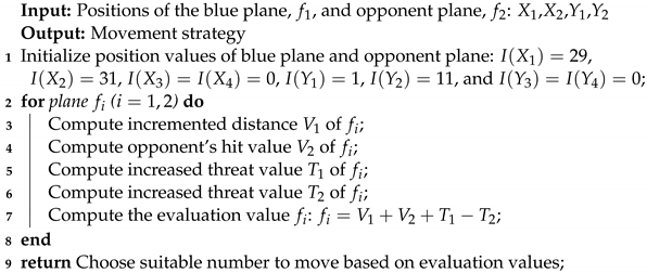
4. Threat Matrix-Based Movement Strategy

In order for readers to better understand our algorithm, we use the following chess position (as shown in Figure 3) as an example to illustrate how our algorithm operates. In this example, it is assumed that $S=(3,5,0,0,1,11,0,0)$ and $R=3$ and it is blue’s turn to make the choice of its plane.

In this example, there are two blue planes (shown as the third and fifth squares in Figure 3) and two red planes (shown as the first and eleventh squares in Figure 3) on the circle, and all other planes are in their staging areas. The threat matrix-based movement strategy for the plane is shown in Algorithm 1.

Algorithm 1: Threat matrix-based movement strategy for plane.

5. Recursion and Complexity Analysis for Multiple Moves

5.1. Recursive for n Plies

In the algorithm and example described above, we have evaluated only one move for the plane based on the current position, which is somewhat short-sighted. For most chess games, in order to win the game multiple moves need to be considered, and this is true for Chinese Ludo.

As the game rules are the same for both sides, the evaluation function applies to both blue’s planes and red’s planes. The plies of $(S,R)$ are limited because there are only four planes and the number of R can only be 1 to 6, which makes it possible to look multiple moves ahead. This means that we can evaluate the opponent’s planes based on their hypothetical choices and then consider the opponent’s hypothetical assessment.

Let $(S^n,R^n)$ represent the hypothetical position of n moves ahead; we can obtain the evaluation of $n+1$ steps based on $f_i(S^n,R^n)$, denoted by $f_i(S^{n+1},R^{n+1})$. Thus, based on the Equations (1)–(15), we have

$$\begin{array}{c}\hfill f_i(S^{n+1},R^{n+1})=V_1\times f_i(S^n,R^n)+V_2\times f_i(S^n,R^n)+T_1\times f_i(S^n,R^n)+T_2\times f_i(S^n,R^n).\end{array}$$

(16)

It is apparent that Equation (16) is a recursive formula; the initial computation is expressed as Equation (11), with which we can look any number of moves ahead. Although the more moves we look ahead, the more beneficial it is to the blue, the computation cost increases exponentially with the increase in the number of moves. Next, we analyze the relationship between the complexity and the number of moves ahead.

5.2. Complexity Analysis

5.2.1. Computation Complexity of One Move

Let us first look at the computation complexity of evaluating $f_i(S,R)$ based on the current position.

First, according to the evaluation functions in Equations (3) and (4), the calculation of $V_1$ and $V_2$ does not need to consider the opponent’s threat; $X_i$ and $Y_j$, the positions of planes, are both integers and not more than 64, and only judgement and a simple addition operation of the positions are needed. For each side, there are only thirteen special positions. Therefore, to calculate $V_1$ + $V_2$, there are at most 13 + 13 = 26 comparisons of special positions.

Next, according to Equations (7) and (10), the calculation of $T_1$ and $T_2$ mainly involves computing $p(X_i,Y_j)$, which is essentially the comparison of positions.

As the real-time computing and threat matrix are two different methods, we discuss them separately in order to compare their respective advantages and disadvantages.

• Complexity of Real-Time Computing
  Considering the most complicated case, where each of Equations (12) and (13) need to be calculated, Equation (12) includes one comparison and Equation (13) includes eight comparisons, while Equations (14) and (15) include two special cases with special positions; thus, there are at most $(1+8)\alpha$ comparisons. The number of all comparisons is at most $(1+8)+(1+8)\alpha$.
  There are at most four opposing planes in play, and the number of all comparisons is therefore $\beta \times (1+8+\alpha \times (1+8\left)\right)$.
  The above represents the calculation of one blue plane, and the blue player has four planes; the number of comparisons is therefore

  $$\beta \times (2\alpha +\beta \times (1+8+\alpha \times (1+8)))=9\alpha {\beta }^2+9{\beta }^2+2\alpha \beta .$$

  (17)
• Computing Complexity Using Threat Matrix
  According to the definition of the threat matrix, there is no need to calculate $p(X_i,Y_j)$ using Equations (12)–(15) each time, as we can simply look up the pre-calculated matrix. According to Equation (7), we look up the threat matrix twice for each opposing plane. As there are $\beta$ opposing planes, there are at most $2\beta$ search instances. Similarly, according to Equation (10), there are at most $2\beta$ search instances for $T_2$. Then, considering the calculation of $V_1$ and $V_2$, which is $2\alpha$, the full computation for one of blue’s planes is $2\alpha +4\beta$.
  As there are at most four blue planes in play, the maximum computation is

  $$\beta \times (2\alpha +4\beta )=4{\beta }^2+2\alpha \beta .$$

  (18)

Comparing Equation (18) with Equation (17), the computation required for the threat matrix is obviously only $(4{\beta }^2+2\alpha \beta )/(9\alpha {\beta }^2+9{\beta }^2+2\alpha \beta )=7.92\%$ with real-time computing, showing that the computation of the threat matrix is only one-eighth that required by real-time computing. In this game, we use the threat matrix instead of real-time computing.

5.2.2. Complexity of More Moves Ahead/per n Plies

According to Equation (11), each player has four planes; thus, there are at most four cases of S. R takes a value from 1 to 6; thus, the complexity of computing $f_i(S^{n+1},R^{n+1})$ is $6\beta$ instances required to compute $f_i(S^n,R^n)$. Therefore, if we look k moves ahead, $\left(6\beta \right)k$, i.e., the computation complexity is $O\left(\right(6\beta \left)k\right)$.

Using the real-time computing method, the complexity is $9\alpha {\beta }^2+9{\beta }^2+2\alpha \beta$, according to Equation (17). If we look one move ahead, the computation is $(9\alpha {\beta }^2+9{\beta }^2+2\alpha \beta )\times 6\beta$, and if we look k steps forward, the computation complexity will be O($(54\alpha {\beta }^3+54{\beta }^3+2\alpha {\beta }^2)k$);

When using the threat matrix, according to Equation (18) the computation is $4{\beta }^2+2\alpha \beta$. If we look one-step forward, the computation is $(4{\beta }^2+2\alpha \beta )\times 6\beta$, and if we look k steps forward, the computation complexity will be O($(24{\beta }^3+12\alpha {\beta }^2)k$);

It is apparent that there is a clear advantage when using the threat matrix, especially in multiple recursions, which we validate in the following experimental section.

6. Experiment Validation

The development of the Chinese Ludo game used an 80 × 86 SCM 32-bit single board computer with a 100 MHz CPU. Because the computing power was very limited, we used the threat matrix and evaluated only one move ahead of the current position. For more advanced game players, we have developed a more complex two-layer recursive algorithm which can evaluate two moves ahead. We used the 32-bit Windows XP OS as the development platform because the game was eventually expected to run on the 80 × 86 32-bit microprocessor. In addition, we chose Microsoft Visual C as the programming language for easier adoption.

To verify the effectiveness of our algorithms, we carried out three groups of experiments to contrast human play versus the machine, evaluation of one move ahead versus two moves ahead, and real-time computing versus using the threat matrix.

6.1. Contrasting Results for Human versus Machine Play

When the development of the game had finished, a team of 50 players was assigned to play against the machine. The whole test lasted for about one month during which there were more than 15,000 matches played, including 5000 matches with no time limit, 5000 matches with a 10 s limit, and 5000 matches with a 5 s limit. The time limit is the maximum time allowed before reacting after the dice are rolled. It was proposed by the company to increase fun and accelerate the game speed. Figure 4 shows the match results. Figure 5 shows the contrast in reaction times between human players and the machine.

From Figure 5, the following can be seen:

• Aside from the randomness of dice rolling, the machine is much smarter than humans at this game. Even without the time limit, the winning rate of human players is only 12%. When there is a 10 s time limit, human players win 7% of the time, and when there is a 5 s time limit, human players only win 2% of the time. In addition, from the comparison of reaction times human players takes eight times as long to play as the machine does.
• When reaction time was limited, human players perform much worse and had much less of a chance (less than one quarter) of winning compared with the machine, which indicates that the decision of human players is rushed. Interestingly, through repeated training certain people were able to make more careful judgements within the 5 s time limit.
• Figure 5 shows the comparison of reaction times between a typical human player and the machine. From Figure 5, it can be seen that the threat matrix has a disadvantage compared with human player, namely, that the reaction time of the machine is proportional to the number of planes in play. Thus, the increase in the time spent with the increase in the number of steps is smooth, and there are no fast decisions. However, this is very different for humans. Although it generally takes human players longer, this does not increase in a strictly monotonic fashion, and at times human players make exceptionally fast decisions. Sometimes, the human player spends much less time than her/his average time, or even less than the machine (for example, at 29 steps, 46 steps and 54 steps). The reason for this is there are special positions, such as hit, dotfly, and jump, where human players can make quick decisions without calculation, whereas a machine must evaluate all planes and then make a choice by comparing evaluation functions. In this particular case, the algorithm can be improved. However, the special positions require extra judgments that take up additional memory space and CPU time. After balancing the potential improvements against the resources required, the company abandoned the optional improvements.

6.2. Comparison of One Move Ahead and Two Moves Ahead

Obviously, for different positions $(S,R)$, the amount of computation is likely to be different, which leads to different levels of computational complexity. This indicates that the evaluations of one move and multiple moves are not comparable. To show the pros and cons of evaluating one move and two moves, we must compare $(S,R)$ at the same position. Thus, we set up twenty different typical positions $(S,R)$ in order to evaluate the difference. Figure 6a shows the comparison of the evaluation result, f, and Figure 6b shows the comparison of the evaluation times.

From Figure 6a, two evaluations are consistent. In order to see their impact on the selection of planes, we created the following formula:

$$\mu (i,j)=\frac{\parallel f_i^1(S,R)-f_i^2(S,R)\parallel }{\parallel f_i^1(S,R)-f_j^1(S,R)\parallel },$$

(19)

where $f_i^1(S,R)$ and $f_i^2(S,R)$ represent the evaluation of the number i plane at one move ahead and at two moves ahead, respectively. Similarly, $f_j^1(S,R)$ represents the evaluation of the number j plane at one move ahead.

In Equation (19), if $\mu (i,j)\ge 1$, it indicates that the difference between the evaluations of one move and two moves of the same plane is larger than those of one move of two different planes. Therefore, the choice of planes at the same position will be different. Otherwise, if $\mu (i,j)<1$, it means that the evaluations of one move ahead and two moves ahead will not change the choice of planes. According to Equation (19), we calculate $\mu (i,j)$ for the twenty positions, as shown in

Table 3. $\mu (i,j)$ for twenty different chess positions $(S,R)$. The * in the table means blank, indicating that the opponent’s plane is in the staging area.

(S, R)	1	2	3	4	5	6	7	8	9	10	11	12	13	14	15	16	17	18	19	20
$\mu (2,1)$	0.21	0.32	0.23	0.14	0.52	0.27	0.54	0.21	0.35	0.12	0.42	0.19	0.51	0.72	0.43	0.62	0.75	0.21	*	0.46
$\mu (2,3)$	0.17	0.13	0.03	0.41	0.12	0.07	0.27	0.24	0.15	0.02	0.12	0.29	0.31	0.25	0.03	0.02	0.15	0.41	0.65	0.07
$\mu (2,4)$	0.31	0.21	0.10	0.21	0.22	0.08	0.23	0.53	0.81	0.02	0.33	0.13	*	*	0.07	0.12	0.60	0.02	0.36	0.21

.

In addition to the above twenty positions, we compared another fifty positions which provided a consistent result, i.e., the evaluation of two moves ahead did not change the choice of planes based compared to the evaluation of one move ahead. In fact, by looking at Equation (16), cited below, we can find the theoretical reasons for this:

$$\begin{array}{c}\hfill f_i(S^{n+1},R^{n+1})=V_1\times f_i(S^n,R^n)+V_2\times f_i(S^n,R^n)+T_1\times f_i(S^n,R^n)+T_2\times f_i(S^n,R^n).\end{array}$$

(20)

In the evaluation of two moves ahead, the two moves need two more rolls of the dice; however, these are hypothetical. Thus, the further evaluation of the second move ahead is evaluated under the weight of $1/6\times 1/6=1/36$, which makes the impact on the further evaluation small. We can see that this is different from other forms of chess.

However, from Figure 6b, the time cost of evaluating two moves ahead is twenty times of that of evaluating one move ahead. In addition, the memory consumption is increased by a large amount.

6.3. Comparison of Real-Time Computing and the Threat Matrix

In order to compare real-time computing and the threat matrix, we conducted experiments using a 32-bit Windows XP platform.

According to the game rules, the results of dice rolling is random, which means that it is hard to acquire the same position (i.e., the initial conditions for the computation) to compare the two evaluations. Therefore, similar to the previous comparison in Section 5.2, we set typical chess positions in order to ensure the consistency of the initial conditions. The results are shown in Figure 7.

It can be seen from the results that the time consumption of evaluation using the threat matrix takes no more than 0.001 s, while the average time when using real-time calculation is 0.008 s, which is highly unstable compared to the threat matrix. The memory consumption of real-time computation is far greater than that of the threat matrix as well.

7. Conclusions

High-performance computers have significantly contributed to the development of artificial intelligence in the gaming industry, however, this should not be a reason to ignore the effort of pursuing a perfect evaluation method. This paper presents a Chinese Ludo program. Unlike most chess programs, which depend on high machine performance, the evaluation function in our program is only a linear sum of four factor values. The other contribution of this research is that we innovatively constructed a threat matrix that allows us to easily acquire the threat between any two dice on any two positions. The threat matrix approach can greatly reduce the amount of calculation, which allows the program to run on a 32-bit 80 × 86 SCM with a 100 MHz CPU while supporting a recursive algorithms to search plies. Our results show that, when compared with the real-time computing, our threat matrix approach can reduce computation costs by nearly 90%. Furthermore, the memory consumption is both reduced and relatively stable, which speeds up evaluation by 58%.

References

1. Danilovic, S.; de Voogt, A. Making sense of abstract board games: Toward a cross-ludic theory. Games Cult. 2021, 16, 499–518. [Google Scholar] [CrossRef]
2. Abdalzaher, M.S.; Muta, O. A Game-Theoretic Approach for Enhancing Security and Data Trustworthiness in IoT Applications. IEEE Internet Things J. 2020, 7, 11250–11261. [Google Scholar] [CrossRef]
3. Silver, D.; Huang, A.; Maddison, C.J.; Guez, A.; Sifre, L.; Van Den Driessche, G.; Schrittwieser, J.; Antonoglou, I.; Panneershelvam, V.; Lanctot, M.; et al. Mastering the game of Go with deep neural networks and tree search. Nature 2016, 529, 484–489. [Google Scholar] [CrossRef] [PubMed]
4. Silver, D.; Hubert, T.; Schrittwieser, J.; Antonoglou, I.; Lai, M.; Guez, A.; Lanctot, M.; Sifre, L.; Kumaran, D.; Graepel, T.; et al. A general reinforcement learning algorithm that masters chess, shogi, and Go through self-play. Science 2018, 362, 1140–1144. [Google Scholar] [CrossRef] [PubMed] [Green Version]
5. Polese, J.; Sant’Ana, L.; Moulaz, I.R.; Lara, I.C.; Bernardi, J.M.; Lima, M.D.d.; Turini, E.A.S.; Silveira, G.C.; Duarte, S.; Mill, J.G. Pulmonary function evaluation after hospital discharge of patients with severe COVID-19. Clinics 2021, 76. [Google Scholar] [CrossRef] [PubMed]
6. Zhang, Z.; Ning, H.; Shi, F.; Farha, F.; Xu, Y.; Xu, J.; Zhang, F.; Choo, K.K.R. Artificial intelligence in cyber security: Research advances, challenges, and opportunities. Artif. Intell. Rev. 2021, 55, 1029–1053. [Google Scholar] [CrossRef]
7. Fu, Y.; Li, C.; Yu, F.R.; Luan, T.H.; Zhang, Y. A survey of driving safety with sensing, vehicular communications, and artificial intelligence-based collision avoidance. IEEE Trans. Intell. Transp. Syst. 2021, 1–22. [Google Scholar] [CrossRef]
8. Morandin, F.; Amato, G.; Gini, R.; Metta, C.; Parton, M.; Pascutto, G.C. SAI a Sensible Artificial Intelligence that plays Go. In Proceedings of the 2019 International Joint Conference on Neural Networks (IJCNN), Budapest, Hungary, 14–19 July 2019; IEEE: Piscataway, NJ, USA, 2019; pp. 1–8. [Google Scholar]
9. Nilsson, A.; Smith, S.; Ulm, G.; Gustavsson, E.; Jirstrand, M. A performance evaluation of federated learning algorithms. In Proceedings of the Second Workshop on Distributed Infrastructures for Deep Learning, Rennes, France, 10 December 2018; Association for Computing Machinery: New York, NY, USA, 2018; pp. 1–8. [Google Scholar]
10. Nkambule, M.S.; Hasan, A.N.; Ali, A.; Hong, J.; Geem, Z.W. Comprehensive evaluation of machine learning MPPT algorithms for a PV system under different weather conditions. J. Electr. Eng. Technol. 2021, 16, 411–427. [Google Scholar] [CrossRef]
11. Shayesteh, S.; Nazari, M.; Salahshour, A.; Sandoughdaran, S.; Hajianfar, G.; Khateri, M.; Yaghobi Joybari, A.; Jozian, F.; Fatehi Feyzabad, S.H.; Arabi, H.; et al. Treatment response prediction using MRI-based pre-, post-, and delta-radiomic features and machine learning algorithms in colorectal cancer. Med. Phys. 2021, 48, 3691–3701. [Google Scholar] [CrossRef] [PubMed]
12. Paveglio, T.B. From Checkers to Chess: Using Social Science Lessons to Advance Wildfire Adaptation Processes. J. For. 2021, 119, 618–639. [Google Scholar] [CrossRef]
13. Torrado, R.R.; Bontrager, P.; Togelius, J.; Liu, J.; Perez-Liebana, D. Deep reinforcement learning for general video game ai. In Proceedings of the 2018 IEEE Conference on Computational Intelligence and Games (CIG), Maastricht, The Netherlands, 14–17 August 2018; IEEE: Piscataway, NJ, USA, 2018; pp. 1–8. [Google Scholar]
14. Zhu, J.; Villareale, J.; Javvaji, N.; Risi, S.; Löwe, M.; Weigelt, R.; Harteveld, C. Player-AI Interaction: What Neural Network Games Reveal About AI as Play. In Proceedings of the 2021 CHI Conference on Human Factors in Computing Systems, Yokohama, Japan, 8–13 May 2021; Association for Computing Machinery: New York, NY, USA, 2021; pp. 1–17. [Google Scholar]
15. Lee, C.S.; Tsai, Y.L.; Wang, M.H.; Kuan, W.K.; Ciou, Z.H.; Kubota, N. AI-FML Agent for Robotic Game of Go and AIoT Real-World Co-Learning Applications. In Proceedings of the 2020 IEEE International Conference on Fuzzy Systems (FUZZ-IEEE), Glasgow, UK, 19–24 July 2020; pp. 1–8. [Google Scholar]
16. Lüscher, T.F.; Lyon, A.; Amstein, R.; Maisel, A. Artificial intelligence: The pathway to the future of cardiovascular medicine. Eur. Heart J. 2022, 43, 556–558. [Google Scholar] [CrossRef] [PubMed]
17. Feng, X.; Slumbers, O.; Wan, Z.; Liu, B.; McAleer, S.; Wen, Y.; Wang, J.; Yang, Y. Neural auto-curricula in two-player zero-sum games. In Proceedings of the Thirty-Fifth Conference on Neural Information Processing Systems (NeurIPS 2021), Virtual, 6–14 December 2021. [Google Scholar]
18. Bošanskỳ, B.; Lisỳ, V.; Lanctot, M.; Čermák, J.; Winands, M.H. Algorithms for computing strategies in two-player simultaneous move games. Artif. Intell. 2016, 237, 1–40. [Google Scholar] [CrossRef] [Green Version]
19. Nangrani, S.; Nangrani, I.S. Artificial Intelligence Based State of Charge Estimation of Electric Vehicle Battery. In Smart Technologies for Energy, Environment and Sustainable Development; Springer: Berlin/Heidelberg, Germany, 2022; Volume 2, pp. 679–686. [Google Scholar]
20. Hankey, A. Kasparov versus Deep Blue: An Illustration of the Lucas Gödelian Argument. Cosm. Hist. J. Nat. Soc. Philos. 2021, 17, 60–67. [Google Scholar]
21. Silver, D.; Schrittwieser, J.; Simonyan, K.; Antonoglou, I.; Huang, A.; Guez, A.; Hubert, T.; Baker, L.; Lai, M.; Bolton, A.; et al. Mastering the game of go without human knowledge. Nature 2017, 550, 354–359. [Google Scholar] [CrossRef] [PubMed]
22. Bai, W.; Cao, Y.; Dong, J. Research on the application of low-polygon design to Chinese chess: Take the Chinese chess “knight” as an example. In Proceedings of the 2021 the 3rd World Symposium on Software Engineering, Xiamen, China, 24–26 September 2021; pp. 199–204. [Google Scholar]
23. Ma, X.; Shang, T. Study on Traditional Ethnic Chess Games in Gansu Province: The Cultural Connotations and Values. Adv. Phys. Educ. 2021, 11, 276–283. [Google Scholar]
24. He, H. The Race Card: From Gaming Technologies to Model Minorities by Tara Fickle. J. Asian Am. Stud. 2021, 24, 515–517. [Google Scholar] [CrossRef]
25. Tomašev, N.; Paquet, U.; Hassabis, D.; Kramnik, V. Assessing game balance with AlphaZero: Exploring alternative rule sets in chess. arXiv 2020, arXiv:2009.04374. [Google Scholar]
26. Available online: https://en.wikipedia.org/wiki/AeroplaneChess (accessed on 1 April 2022).
27. Polk, A.W.S. Enhancing AI-based game playing using Adaptive Data Structures. Ph.D. Thesis, Carleton University, Ottawa, ON, Canada, 2016. [Google Scholar]
Figure 1. The chessboard of the Chinese Ludo game.
Electronics 11 01699 g001
Figure 2. The definition of a chess position on the chessboard.
Electronics 11 01699 g002
Figure 3. An example with chess position ( S , R ) , where S = ( 3 , 5 , 0 , 0 , 1 , 11 , 0 , 0 ) and R = 3 .
Electronics 11 01699 g003
Figure 4. Contrast in match results between humans and machine: (a) statistics on the match results; (b) comparison of wins.
Electronics 11 01699 g004
Figure 5. Comparison of reaction time between humans and machine.
Electronics 11 01699 g005
Figure 6. Comparison of the evaluation of one move and two moves ahead. The vertical axis indicates the evaluation results, f, in (a) and indicates the evaluation time in (b).
Electronics 11 01699 g006
Figure 7. Comparison of real-time computing and the threat matrix in terms of time complexity and memory usage: (a) comparison of time complexity; (b) comparison of memory usage.
Electronics 11 01699 g007