Article

Understanding the Sources of Ambient Fine Particulate Matter (PM2.5) in Jeddah, Saudi Arabia

1
Department of Environmental Health Sciences, School of Public Health, University at Albany, Albany, NY 12201, USA
2
Wadsworth Center, New York State Department of Health, Albany, NY 12201, USA
3
Unit for Ain Zubaida Rehabilitation and Ground Water Research, King Abdul-Aziz University, P.O. Box 80200, Jeddah 21589, Saudi Arabia
4
Department of Environmental and Health Research, The Custodian of the Holy Two Mosques Institute for Hajj and Umrah Research, Umm Al-Qura University, P.O. Box 6287, Makkah al Mukarramah 21955, Saudi Arabia
5
Institute for the Health & the Environment, University at Albany, Rensselaer, NY 12144, USA
6
Department of Chemistry, University of California, Irvine, CA 92617, USA
*
Author to whom correspondence should be addressed.
Atmosphere 2022, 13(5), 711; https://doi.org/10.3390/atmos13050711
Submission received: 30 March 2022 / Revised: 23 April 2022 / Accepted: 27 April 2022 / Published: 29 April 2022
(This article belongs to the Special Issue Outdoor Air Pollution and Human Health (2nd Edition))

Abstract

:
Urban air pollution is rapidly becoming a major environmental problem of public concern in several developing countries of the world. Jeddah, the second-largest city in Saudi Arabia, is subject to high air pollution that has severe implications for the health of the exposed population. Fine particulate matter (PM2.5) samples were collected for 24 h daily, during a 1-year campaign from 2013 to 2014. This study presents a detailed investigation of PM2.5 mass, chemical composition, and sources covering all four seasons of the year. Samples were analyzed for black carbon (BC), trace elements (TEs), and water-soluble ionic species (IS). The chemical compositions were statistically examined, and the temporal and seasonal patterns were characterized using descriptive analysis, correlation matrices, and elemental enrichment factor (EF). Source apportionment and source locations were performed on PM2.5 samples using the positive matrix factorization (PMF) model, elemental enrichment factor, and air-mass back trajectory analysis. The 24-h mean PM2.5 and BC concentrations ranged from 33.9 ± 9.1–58.8 ± 25 µg/m3 and 1.8 ± 0.4–2.4 ± 0.6 µg/m3, respectively. Atmospheric PM2.5 concentrations were well above the 24-h WHO guideline of 15 µg/m3, with overall results showing significant temporal and seasonal variability. EF defined two broad categories of TEs: anthropogenic (Ni, V, Cu, Zn, Cl, Pb, S, Lu, and Br), and earth-crust derived (Al, Si, Mg, K, Ca, Ti, Cr, Mn, Fe, and Sr). The five identified factors resulting from PMF were (1) fossil-fuels/oil combustion (45.3%), (2) vehicular emissions (19.1%), (3) soil/dust resuspension (15.6%), (4) industrial mixed dust (13.5%), and (5) sea-spray (6.5%). This study highlights the importance of focusing control strategies, not only on reducing PM concentration but also on the reduction of components of the PM as well, to effectively protect human health and the environment.

1. Introduction

Fine particulate (PM2.5) air pollution remains a major issue in Saudi Arabia, attributed largely to heavy industrialization and urbanization [1,2], with no proper policy implementation in place. This has progressively led to poor urban air quality. Over time, the number of both stationary (oil refineries, petrochemical industries, desalinization plants, power generation, etc.), and mobile sources (heavy trucks, buses, cars, etc.) of air pollution have increased tremendously. There was an estimated > 1.4 million cars in Jeddah in 2012 [3].This number has most likely increased over the years. Fine particulate (PM2.5) emissions from these sources significantly affect air quality.
Indeed, a few studies [1,2,3,4] assessing PM2.5 air pollution in Saudi Arabia’s major cities reported poor air quality, mainly linked to industrial and vehicular emissions. Overall, there is a major consensus that anthropogenic sources contribute significantly to the observed air pollution in Saudi Arabia. The World Health Organization (WHO) recommends annual, and 24-h mean PM2.5 at 5 and 15 μg/m3, respectively [5]; and the Presidency of Meteorology and Environment (PME) of Saudi Arabia regulates PM2.5 at 15 and 35 μg/m3 annual and 24-h mean, respectively [6]. Most of the studies done in Saudi Arabia’s major cities [1,2,7,8] showed evidence of PM2.5 levels exceeding both the PME and WHO guidelines, as well as the levels recorded in Europe [9,10,11,12] and North America [13,14,15,16].
In addition, mounting evidence from several epidemiologic studies has shown that exposure to fine particulate air pollution, at much lower levels than reported in this study, significantly increases the risk of morbidity and mortality from cardiopulmonary diseases [17,18,19,20], and exacerbates pre-existing medical conditions such as asthma, coronary obstructive pulmonary disease [21,22], and other illnesses, notably among children and the elderly. Given the extent of the adverse health outcomes reported at much lower PM2.5 levels, this further accentuates the need for more studies assessing air quality in Saudi Arabia and the rest of the Middle East. This study becomes one of the pioneer studies to fully characterize the state of air quality in Jeddah, providing a breakdown on the major emission sources.
The chemical and physical characterization of PM2.5 is key to understanding its toxicity, as well as elucidating more on the possible emission sources. This is critical to the design and implementation of more effective policies, and ultimately, the preservation of human health and the environment. For Jeddah, being one of the major industrialized cities in Saudi Arabia, results from this study will be fundamental to the improvement of existing local and regional policies on air pollution, mainly targeting the major anthropogenic sources. This study addresses four main objectives: (1) providing a detailed assessment of the levels of ambient PM2.5, black carbon (BC), trace elements, and water-soluble ionic species; (2) discussion of the temporal and seasonal variabilities in air pollution levels and composition; (3) source apportionment using factor analysis approaches (elemental enrichment factor and positive matric factorization); and (4) discussion of some of the suggested recommendations for current and future air pollution control in Jeddah and other cities in the region.

2. Materials and Methods
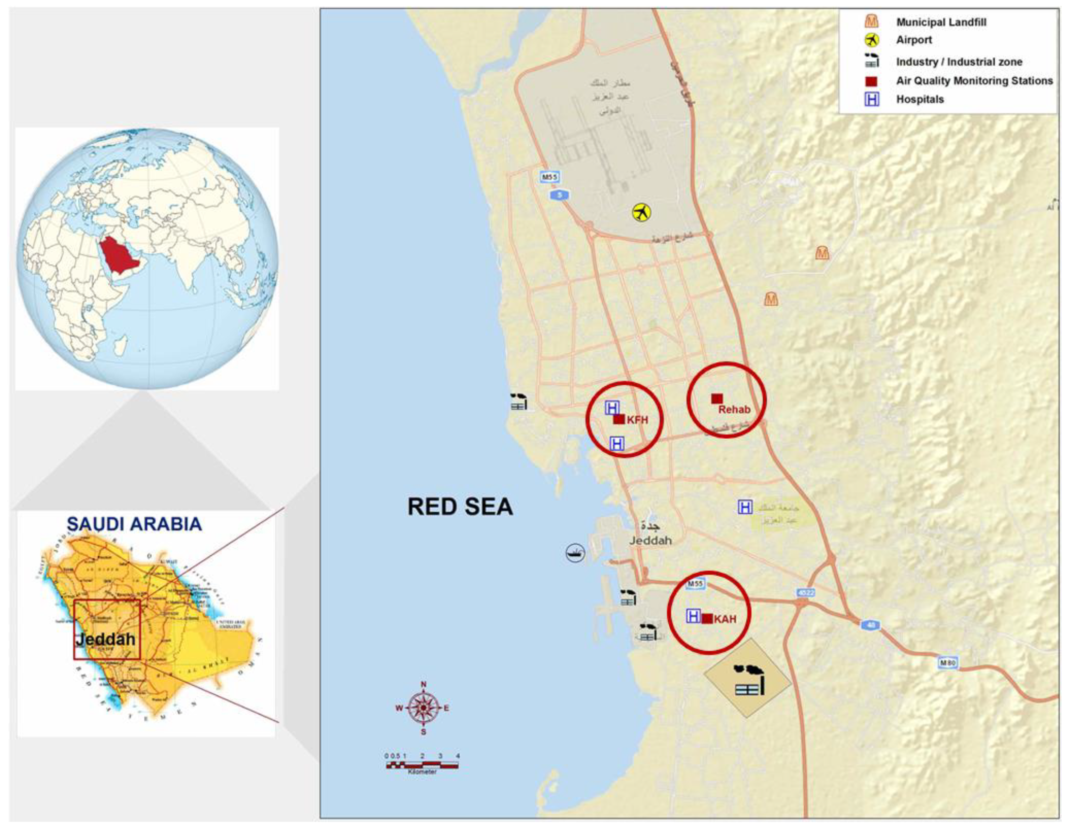
2.1. Study Area

Jeddah city (Figure 1) is the second-largest city in Saudi Arabia, located in the Hijaz Tihamah region (Lat. 21.3° North and Lon. 39.2° East), midway eastern shore of the Red Sea. The city has a municipality area of 5460 km2 and population of 3.98 million people [23]. Jeddah features a semi-arid to arid climate [24]. Rainfall only occurs around November to January, with an annual mean of 44.6 mm (http://www.holiday-weather.com/jeddah/averages/ accessed on 4 May 2021). The city is characterized by heavily industrialized areas with different types of industries (such as oil refineries, desalination, iron smelting, etc.), heavy vehicular traffic, and sandstorms.
Due to its location, Jeddah’s prevailing winds are frequently northwesterly. During winter, spring, and fall, blustery winds also blow from the south, causing sandstorms, sometimes accompanied by thunderstorms and heavy rains [24]. Winters are warm, from 15–18 °C at dawn to ≥28 °C in the afternoon. Summers are hot and humid (≥40 °C in the afternoon and ≥31 °C in the evening). These weather conditions directly influence the levels of PM2.5. More climate information on Jeddah can be found at: http://www.jeddah.climatemps.com/ (accessed on 4 May 2021).

2.2. PM2.5 Sampling and Analysis

PM2.5 samplers were installed at three fixed sampling sites (Figure 1). Sampling was done for six weeks in each quarter of the year starting from 8 April 2013–18 February 2014. Each quarter represented a sampling cycle. The first and second cycles were sampled at King Abdul-Aziz Hospital (KAH) and King Fahad Hospital (KFH), while the third and fourth were at KAH and Al-Rehab/or KAU (King Abdul-Aziz University) sites. The first 10 days of cycle 1 were sampled at Al-Rawda, and the rest at the KFH site. These sampling sites were selected in such a way as to represent a relatively uniform blend of residential and industrial areas. Residential sites were densely populated areas, while the heavy traffic and industrial areas represented industrial sites. This resulted in a representative mix for both the residential and industrial areas, and thus, a more accurate estimation of the actual pollution levels in real time. Meteorology data were obtained online from https://www.wunderground.com (accessed on 4 May 2021).
The 24-h PM2.5 samples were collected on pre-weighed, sequentially labeled Whatman 46.2 mm diameter 2.0 μm pore polytetrafluoroethylene (PTFE) filters (Whatman plc, Florham Park, NJ, USA) using a low volume air sampling pump (VS23 series pump, HI-Q Environmental Products Company, Inc., San Diego, CA, USA). The PM2.5 sampler (Figure S1) was equipped with a cyclone separator with a cut size of 2.5 µm operated at a flow rate 16.7 ± 0.84 L/min, optimum for sampling the PM2.5 size range. The sampler inlets were fixed at about 5 m above the ground for a good representation of ambient PM2.5 and to avoid influence of ground dust. The sampled filters were stored in labeled clean polypropylene petri-dishes and immediately refrigerated at 4 °C to minimize further loss of temperature sensitive ammonium, nitrate, and oxalate. At the end of the sampling cycle, all the samples were shipped to the Wadsworth Center, New York State Department of Health, Albany, NY, USA, to be analyzed for PM2.5 levels, black carbon (BC), trace elements (TEs), and water-soluble ionic species. The samples were refrigerated until analysis. Given the large number of samples corrected, analysis for the different pollutants was completed within 3–4 months of receiving the samples.
The 24-h PM2.5 levels were determined gravimetrically as the difference of the PTFE filter weight before and after sampling. BC loading (μg/m3) on the filters was determined using a dual-wavelength Optical Transmissometer (Model OT-21, 2007), Magee Scientific, Francisco St, Berkeley, CA, USA. The OT-21 collects absorbance data at 370 nm and 880 nm wavelengths. To correct for the loading effects, we applied attenuation coefficients K880nm = 16.6 m2 g−1 and K370nm = 39.5 m2 g−1 [25] at respective channels. The difference between BC370nm and BC880nm estimates delta–C (Equation (1)), a marker for organic matter combustion [26,27].
Delta–C = BC370nm − BC880nm
TEs were analyzed by an energy dispersive X-ray fluorescence (ED–XRF) spectrometer (Thermo Scientific™, Waltham, MA, USA) using six secondary fluorescers (Si, Ti, Fe, Cd, Se, and Pb). ED–XRF has been extensively used for TEs analysis in air particulate samples [28,29,30] because it is fast and does not require chemical digestion of samples prior to analysis [31], which minimizes contamination. This technique works on a principle that distinct atoms, when excited by an external high energy, will emit X-ray photons with characteristic energy and wavelengths. So, TEs in a sample can be identified and quantified by measuring the intensity of photons of each energy emitted from the sample [32,33]. The intensity of radiation signal from each TE in the sample, which is also proportional to its concentration, is then computed from a set of internal calibration curves.
The water-soluble ionic species were analyzed using ion-exchange chromatography (IC) (Dionex, Sunnyvale, CA, USA). A summary of the optimized conditions used for the analysis of water-soluble ionic species by IC, has been included in the Supplemental Materials (Table S1). Strict quality control and quality assurance measures were taken throughout the study. Typical detection limits of trace elements measured in this study are provided in Supplemental Materials (Table S2, based on [34]). More details of the sampling and analyses for PM2.5 levels, BC, TEs, and ionic species have been previously provided [1,7].

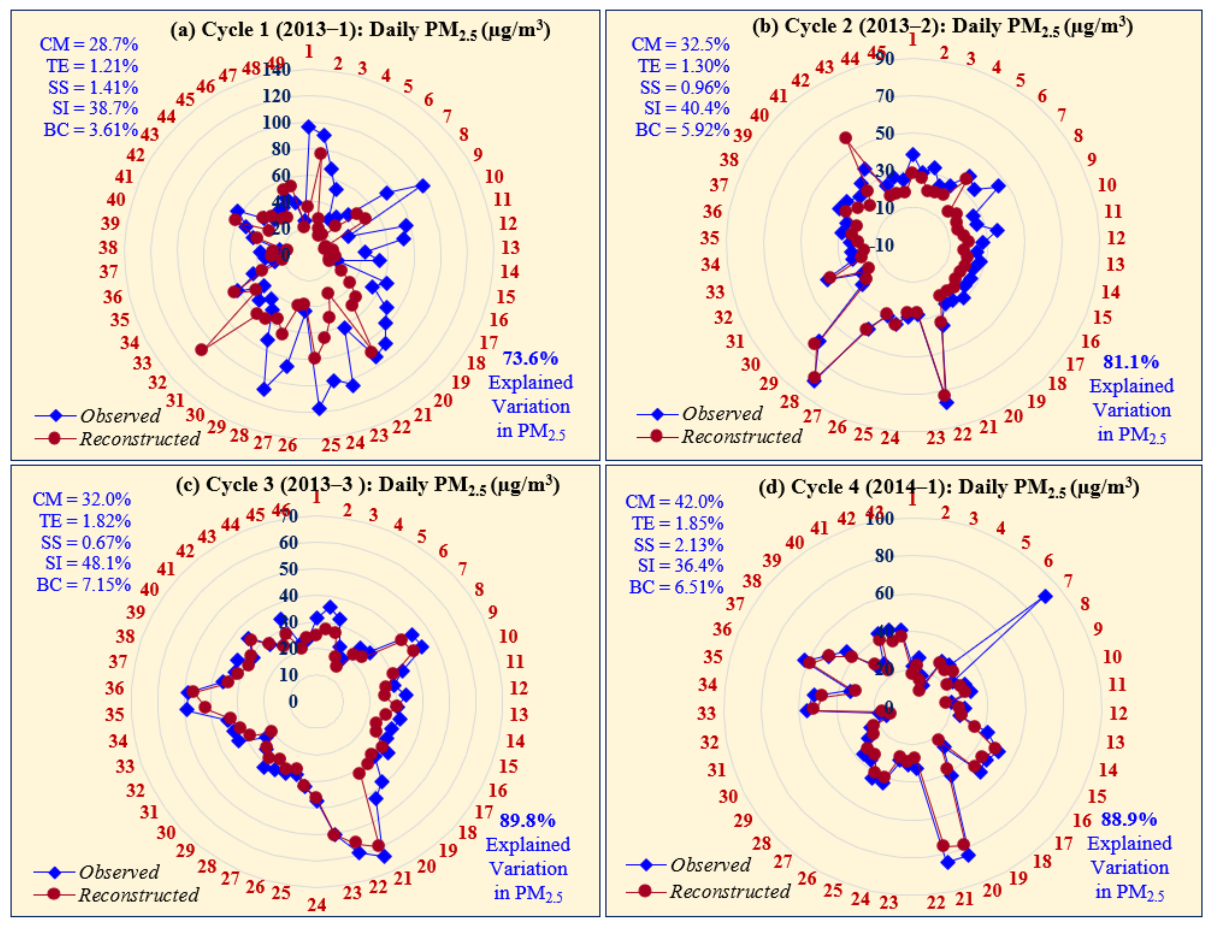
2.3. PM2.5 Mass-Reconstruction

We performed PM2.5 mass-reconstruction by re-grouping the chemical species measured in PM2.5 aerosol into six major categories [1]: (1) crustal/geological materials; (2) anthropogenic trace elements (TEs); (3) secondary inorganic ions (IS) (SO42−, NO3, NH4+, and C2O42−); (4) sea salt/sea sprays; (5) black carbon (BC)/soot; and (6) particulate organic matter (POM). These categories makeup the proportion of the overall PM2.5 explained by the measured pollutant species in our analyses [35]. Additional details on the frequently applied mass-reconstruction equations and the backgrounds and assumptions related to each pollutant category can be found in several previous studies [35,36]. The reconstructed PM2.5 mass was calculated as shown in Equation (2):
Reconstructed PM2.5 = Crustal Material [CM] + Trace Elements [TE] + Sea Spray [SS] + Secondary Ions [SI] + Elemental Carbon [EC/ or BC] + Organic Matter [OM]
where:
[CM] = 1.89[Al] + 1.21[K] + 1.43[Fe] + 1.4[Ca] + 1.66[Mg] + 1.67[Ti] + 2.14[Si]
[TE] = 1.31[V] + 1.46[Cr] + 1.29[Mn] + 1.27[Ni] + 1.13[Cu] + 1.24[Zn] + 1.32[As] + 1.41[Se] + 1.40[Br] + 1.37[Sr] + 1.14[Er] + 1.12[Ba] + 1.14[Lu] + 1.08[Pb](4) [7,37,38]
[SS] = [Cl] + ss [Na+] + ss [Mg2+] + ss [K+] + ss [Ca2+] + ss [SO42−]
where ss [Na+] = 0.556 [Cl]; ss [Mg2+] = 0.12 ss [Na+]; ss [K+] = 0.036 ss [Na+]; ss [Ca2+] = 0.038 ss [Na+]; and ss [SO42−] = 0.252 ss [Na+]; [39]
[SI] = nss [SO42−] + [NO3] + [NH4] + [C2O42−]
where nss [SO42−] = [SO42−] − ss [SO42−]; ss and nss denote sea spray and non-sea spray, respectively.
The oxide factors used in Equations (3) and (4) were estimated bases on the most stable oxides (Al2O3, K2O, Fe2O3, CaO, MgO, TiO2, SiO2, VO, Cr2O3, MnO, NiO, Cu2O, ZnO, As2O3, SeO2, BrO2, SrO2, Er2O3, BaO, Lu2O3, and PbO) of these elements [7,37,38].

2.4. PM2.5 Source Apportionment

We performed source apportionment for PM2.5 using three approaches; PM2.5 mass-reconstruction, elemental enrichment factor (EF), and positive matrix factorization (PMF). Results were carefully studied from the three approaches to accurately define the sources of PM2.5 in Jeddah.
Enrichment factors (EFs) were calculated using Al as a reference element (Equation (7)) to assess the extent of anthropogenic contributions to the measured PM2.5 levels, as explained in previous studies and some of our past work [26,27].
EF = ( C x / C Al ) PM 2.5 ( C x / C Al ) Earth crust
Cx and CAl denote the levels of the element “x” and “Al”, respectively, in the ambient PM2.5 sample and the earth-crust. The relative abundances of trace elements in the earth-crust were obtained from Taylor (1964). EF values greater than 10 suggest a significant anthropogenic contribution, while EF values less than 10 are indicative of major contributions from the earth-crust. Generally, the EF values between 10 to 50 are indicative of mixture of anthropogenic and earth-crust derived emissions, while EF values greater than 50 are indicative of purely anthropogenic emissions.
To delineate various sources of PM2.5, we used the latest the United States Environmental Protection Agency (U.S.EPA) positive matrix factorization (PMF) receptor model (version 5.0.14). This is a mathematical receptor model that utilizes a multivariate factor analysis to breakdown a complex matrix of well speciated sample data (containing both concentration and uncertainty estimates) into two simpler matrices as factor profiles and factor contributions. Based on the species within each profile, we drew interpretations for the source types using the measured chemical species in the samples as markers for specific sources. More details on PMF analysis and the resolution, interpretation of factors, and the QA/QC measures have been provided in several previous studies [40,41,42].
We utilized the backward-in-time hybrid single-particle Lagrangian integrated trajectories (HYSPLIT) set at an altitude of 500 m above sea level, to determine the direction of air-mass flow. The atmospheric boundary layer (ABL), which is the lowest part of the atmosphere, is about 50 to 3000 m above sea-level [43]. This is the space where most of the anthropogenic activities and meteorological trends occur. Obtaining an accurate estimate of the ABL for a given study area is of a critical importance in air pollution studies. Previously reported data show that the depth of the mixed layer over the Arabian Sea ranges from 400 to 900 m, but with high variability near the shores due to the intricate nature of the interactions between the land and sea breezes [44]. In another study, Jeddah’s ABL was estimated around 900 m, but with some variability [45]. Given the range of ABL estimates around the Arabian Sean and Jeddah, we ran our HYSPLIT models set at 500 m above the sea level because this height provides a representative regional ABL where most anthropogenic activities take place. However, most importantly, the significance of this ABL height is that; (1) it is optimum for long-range atmospheric transport of pollutants, and (2) it has a direct influence on human exposure risk. Pollutants dispersed over 500 m above sea-level will be transported over a much longer distance, but the possibility of human exposure is significantly diminished to almost zero. So, as we assessed the wind trajectories, our focus remained centered around the question of how this influences human exposure. Trajectories covering a period of up to 72 h prior to sampling date were computed to determine the direction of air mass flow into the study area. The plots for backward-in-time trajectories with their respective data files were downloaded from the National Oceanic and Atmospheric Administration (NOAA) website [46,47]. When interpreted correctly, wind trajectories can provide insightful information about the contribution of the regional and local emissions towards the observed levels of PM2.5.

3. Results and Discussion

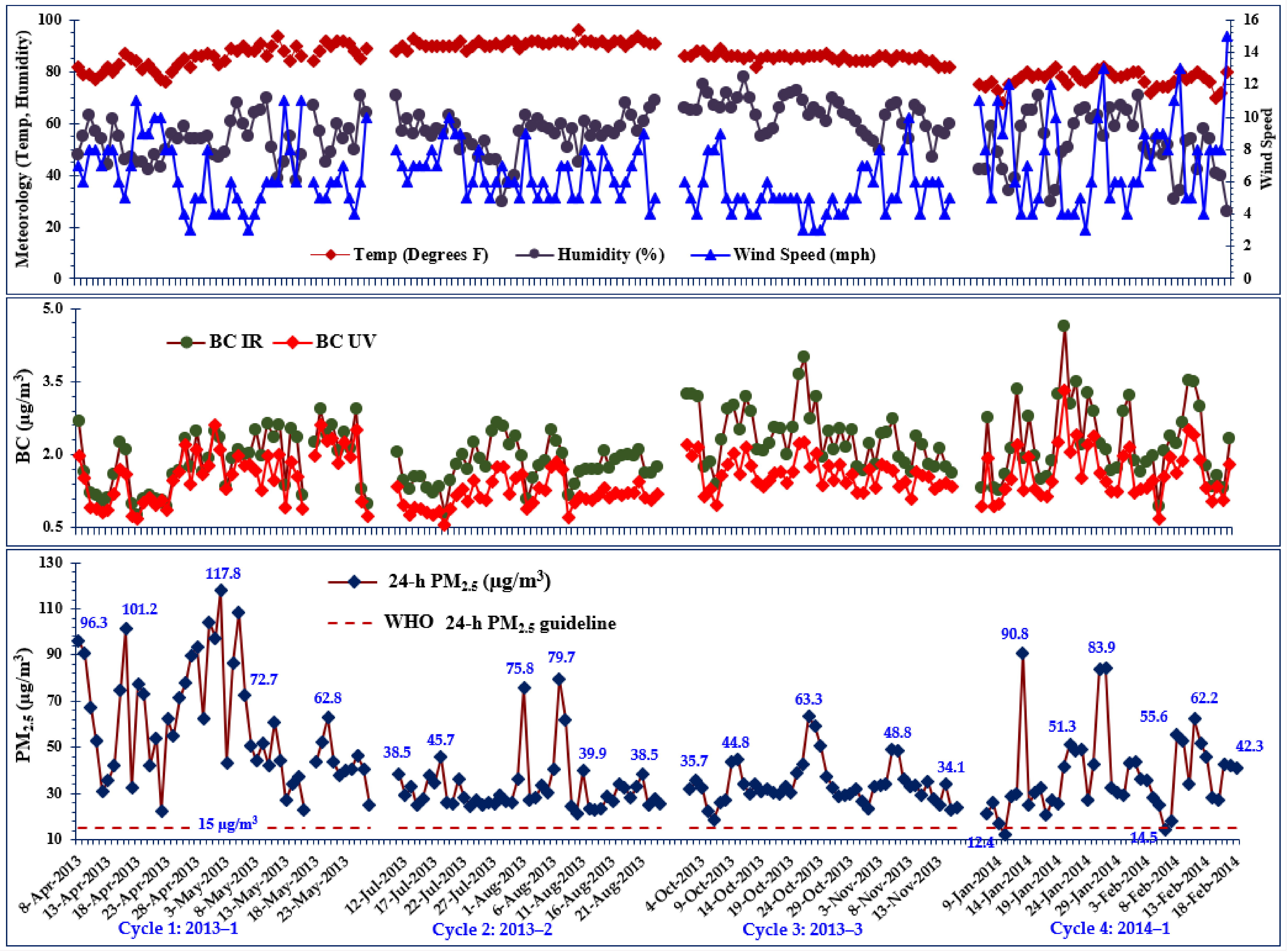
3.1. PM2.5 Mass and Chemical Composition

The mean daily (24-h) PM2.5 and its components (BC, TEs, and IS), and meteorology, are summarized in Table 1. The mean daily temperature was relatively stable (25.0–29.6 °C), while relative humidity (RH) and wind speed (WS) varied significantly throughout the study period (Figure 2). Additionally, the 24-h PM2.5 displayed significant temporal variability with the mean PM levels per cycle, far exceeding the 24-h WHO guideline (25 μg/m3), 91% of the study period (Figure 2). Overall, PM2.5 levels gradually increased around January and February (cycle 4) and was highest in April and May (cycle 1). This seasonal trend may partly be linked to meteorology. Jeddah experiences strong winds and sandstorms during winter and spring [48]. This may account for a significant portion of the high PM2.5 levels recorded during cycles 1 and 4. Moreover, the ambient temperature inversion during winter lowers the atmospheric boundary layer, which in turn limits the dispersion of airborne pollutants. Ultimately, this leads to increased concentration of ambient PM2.5 as observed in this study.
Black carbon (BC) had a significant daily variability but with no major seasonal variability observed (Figure 2). This was linked to BC being mostly associated with vehicular and industrial emissions. Emissions from these sources may fluctuate significantly by the day of the week (weekday–weekend trends), but not by season. BC, as represented by a signal at infra-red λ (BCIR), explained only 3.6–7.2% of the total PM2.5. In addition, the mean delta–C levels per cycle were below zero (Table 1). Only two (2) days in cycle 1 had delta–C ˃ 0 (0.01 and 0.14 μg/m3). Delta–C, computed as the difference in BC measurements at ultraviolet λ (BCUV) and BCIR, is a strong marker for organic matter combustion [26,27]. Thus, the observed results in this study point to a minor or no contribution from biomass burning to the overall recorded PM2.5 levels in Jeddah.
Up to twenty-four (24) trace elements (TEs) were detected at levels above their respective limits of quantification (LOQ), as per the analytical method used (Table 1). Crustal elements (Si, Ca, Fe, Al, and Mg) recorded the highest concentrations, signaling a significant influence from the earth crust/soil. Sulfur (S), Cl, and Na also constituted the most abundant elements. Several anthropogenic TEs (S, Ni, V, Cu, Y, Zn, Cl, S, Pb, Br, Lu, and Ce) were detected. These TEs are intricately linked to vehicular emissions (Pb, Ni, Cu, Br, and Ce), fossil-fuels/oil combustion (S, V, and Lu), and other industrial processes [49,50].
The water-soluble ionic species (IS) were mostly sulfate (SO42−), nitrate (NO3), and ammonium (NH4+), as shown in Table 1. High concentrations of SO42− and NO3 species in the ambient air can be indicative of significant anthropogenic emissions from fossil-fuels/oil combustion (SO42−) and vehicular emissions (NO3).

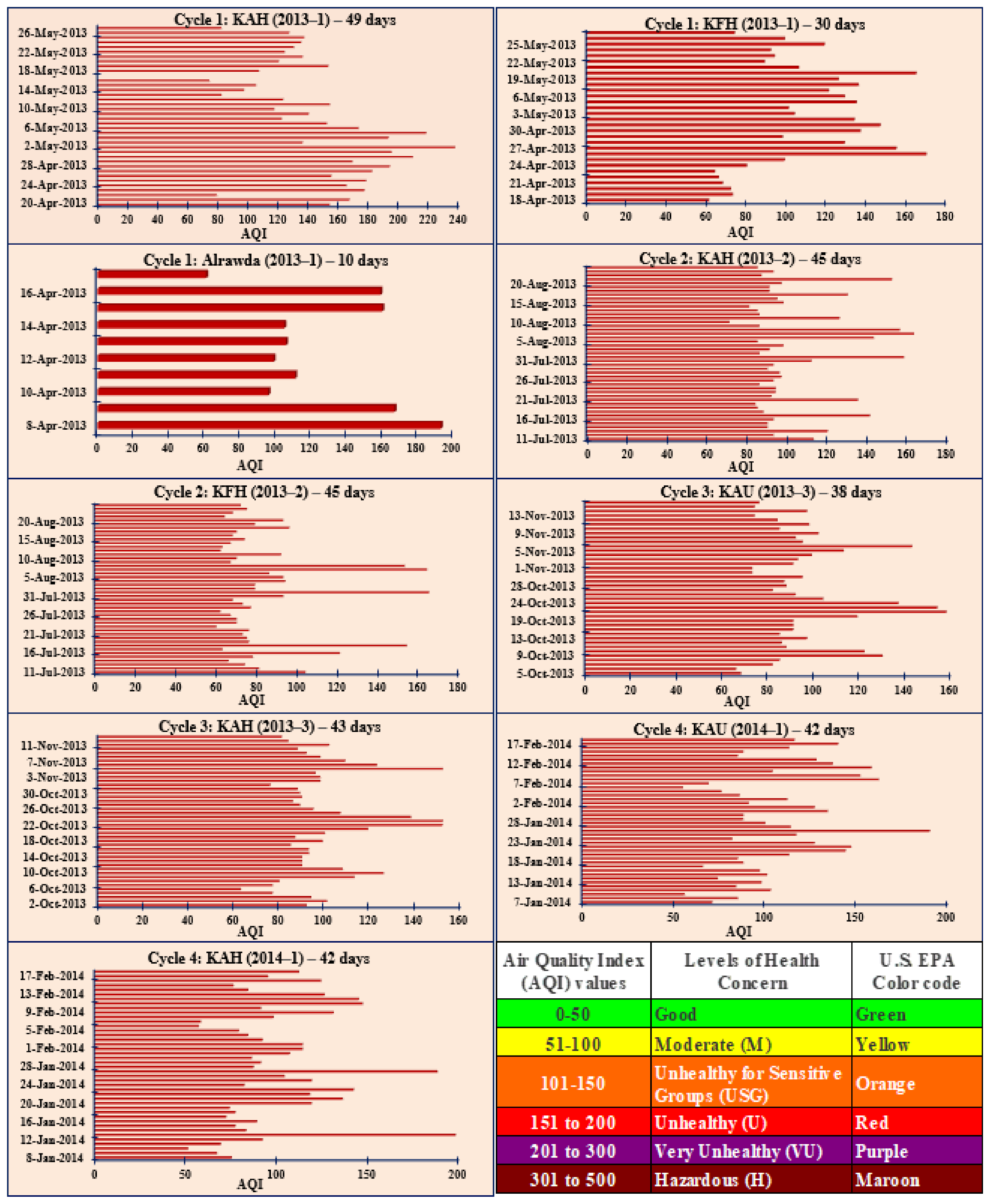
3.2. Air Quality Index (AQI) in Jeddah and Comparison with Other Studies

The AQI was calculated [51] based on the observed daily PM2.5 levels (Figure 3). The calculated AQI for any given pollutant is always proportional to its levels in the air. Thus, the high AQI values, as seen in this study, simply imply elevated levels of ambient PM2.5 in Jeddah. This also translates to a great deal of severe health risk for the exposed population. With exception of cycle 1 that recorded unhealthy to very unhealthy AQI, the general air quality for the rest of the study period was mostly at a moderate level (Figure 3). Notably, we did not observe a single day with good air quality throughout the study period. This further stressed the severity of particulate air pollution in Jeddah and the rest of the Middle East region. Moreover, the AQI in this study was calculated using only the overall PM2.5 levels. Thus, we may have potentially underestimated the severity of the observed air pollution levels. Results could possibly show more severe health effects, if additional AQI values based on the gaseous pollutants, such as ozone (O3) and sulfur dioxide (SO2), were available. It is also noteworthy that, though the AQI provides a simplified interpretation of the health hazard level associated with an exposure to a given air pollutant, it is not an air quality guideline. Nevertheless, the AQI results can inform the process of policy formulation and implementation.
Furthermore, we compared the recorded daily PM2.5 levels with both the WHO and Saudi Arabia’s PME guidelines, and the levels recorded in other cities worldwide. The observed mean 24-h PM2.5 did not only exceed the 24-h WHO (15 μg/m3) and PME (35 μg/m3) guidelines but were also markedly higher than levels reported for most urban centers of developed countries globally (Figure S2, based on [1,11,12,16,52,53,54,55,56,57,58,59,60,61,62,63,64,65]). Only the major cities in developing countries such as India, China, Pakistan, Bangladesh, and Mongolia, that have historically high levels of air pollution, had PM2.5 levels that were either comparable or higher than the levels recorded in this study (Figure S2). This further stressed the extent of particulate air pollution in Jeddah and the rest of the Middle Eastern region.

3.3. PM2.5 Mass-Reconstruction

The PM-mass reconstruction tool was utilized to explain the variations between the observed and the expected PM2.5 levels. Daily PM2.5 was decomposed into five (5) broad pollutants categories as: crustal materials (CMs), secondary ions (SI), sea-sprays (SS), black carbon (BC), and anthropogenic TEs, which we used to explain the variations in daily PM2.5, as presented in Figure 4. Overall, the largest portion (38.7–48.1%) was attributed to SI (SO42−, NO3, and NH4+). The precursors of p-SO42− (SO2) and p-NO3 (NOX) are typically linked to fossil-fuel combustion and vehicular emissions. The second largest portion (28.7–42%) was attributed to CMs, especially during cycle 4 (January–February) where CMs comprised the largest proportion (42%) of the overall PM2.5. Jeddah experiences strong winds accompanied by sandstorms during winter and spring seasons [48]. These drastically increase the ambient enrichment of CMs. BC and the anthropogenic TEs also constituted a significant portion of the measured PM2.5, further highlighting the influence of anthropogenic PM emissions in Jeddah. In general, BC, TEs, and SI combined explained 73.6–89.5% of the observed PM2.5 (Figure 4).
The estimates of particulate organic matter (POM) were not available for this study. In addition, converting the total S from ED-XRF to SO42− (expected) and comparing it with the soluble SO42− from IC analysis (observed), showed significant differences per cycle (Table S3). While cycle 1 over-estimated SO42−, cycles 2–4 showed significant under-estimates of observed SO42−. This may partially be due to some S-containing compounds not being completely water-soluble [36]. The observed SO42 represents only the water-soluble portion. The PM mass closure on SI used the observed SO42−. The remaining water-insoluble portion and POM account for the unexplained portion of PM2.5 during cycles 2–4. Despite the significant over-estimates in SO42−, cycle 1 still had the largest portion of unexplained PM2.5 (26.4%). This may partially be attributed to the missing POM and some measurement errors. Besides being a useful tool for delineation of sources, PM mass-reconstruction can be utilized for assessing the data integrity where significant over- and under-estimates may be revealed by comparing the observed and re-constructed levels of target pollutants, as shown in Figure 4.

3.4. Correlation between Air Pollutants and Meteorology

Correlations (r) between various pollutants are summarized in Table S4. Pearson’s correlation was favored because we wanted to assess the linear relationships between individual pollutant species and meteorology. This is critical to understanding the links between the pollutants measured in PM2.5 aerosol, and ultimately, the accurate delineation of their emission sources. Mean daily PM2.5 had a weak negative correlation with wind speed (WS) (r = −0.24), and temperature (r = −0.13), p-value < 0.0001. WS increases the ambient dispersion of PM2.5, while elevated ambient temperatures cause unstable atmospheres and strong convective winds, leading to quick dispersion of PM2.5; thus, the observed negative correlations.
Daily PM2.5 was moderately correlated (p-value < 0.0001) with crustal TEs; Mg (r = 0.67), Si (r = 0.66), Al (r = 0.63), K (r = 0.57), Ti (r = 0.43), Fe (r = 0.39), and Ca (r = 0.33), indicating a major contribution from the earth crust, as highlighted by the proportion of PM2.5 attributed to CM (Figure 4). In addition, PM2.5 was moderately correlated with anthropogenic TEs; Ni (r = 0.53), Cu (r = 0.48), Lu (r = 0.42), Zn (r = 0.32), and Pb (r = 0.20), p-value < 0.0001. Though these TEs accounted for a small portion (1.2–1.9%) of PM2.5 (Figure 4), they are good makers for specific anthropogenic sources.
Daily PM2.5 had a moderate correlation with p-SO42 (r = 0.50, p-value < 0.0001) and not correlated with p-NO3, indicating a major industrial contribution. Jeddah is heavily industrialized, and thus the high emissions of SO2 are a precursor for the observed high levels of p-SO42 in this study. p-SO42− constituted a major portion of the secondary aerosols (SI).
The daily PM2.5 was moderately correlated with p-NH4+ (r = 0.30), but p-NH4+ was highly correlated with p-SO42− (r = 0.73), p-value < 0.0001. This high correlation between p-NH4+ and p-SO42− is more linked to the fact that both species are mostly formed as fine aerosols, through similar gas-phase reactions, as opposed to having a common source. Moreover, p-NH4+ was evidently less than p-SO42− (Table 1) with a molar ratio (NH4+:SO42−) of 0.24 (<2), implying an incomplete neutralization of ambient H2SO4. Thus, the available NH4+ salts consisted of a mixture of (NH4)2SO4 and NH4HSO4 (Equations (8) and (9)). In addition to the high emission sources, the observed high p-SO42− levels may also be attributed to elevated ambient temperatures, favorable for the photochemical activity and atmospheric oxidation processes; hence, the increased oxidation of SO2 to p-SO42. Besides, there was barely enough NH4+ to neutralize one quarter of the observed p-SO42. Thus, most of the p-SO42 was likely from ionization of atmospheric H2SO4, as shown in Equation (10).
2NH3 (g) + H2SO4 (aq) → (NH4)2SO4 (aq) − likely
NH3 (g) + H2SO4 (aq) → (NH4)HSO4 (aq) − likely
H2SO4 (aq) ↔ H+ (aq) + SO42 (aq) − largest proportion of p-SO42
In addition, p-SO42− was moderately correlated with Ni (r = 0.56), Cu (r = 0.38), Zn (r = 0.35), Lu (r = 0.30), V (r = 0.26), and Pb (r = 0.24), p-value < 0.0001, suggesting both a common source and a portion of the observed p-SO42− existing in the form of sulfates of these anthropogenic TEs.
p-NO3 had a moderate negative correlation with p-NH4+ (r = −0.50), SO42− (r = −0.27), and a positive correlation with Cl (r = 0.39). p-NH4+ and Cl were also negatively correlated (r = −0.32), p-value < 0.0001. These negative correlations are indicative of different temporal variabilities. Additionally, this shows that there was no p-NH4+ attributable to neutralization of atmospheric HNO3 and HCl. Thus, the p-NH4+ salts did not comprise any NH4NO3 and NH4Cl. Positive correlations between p-NH4+, p-SO42−, p-NO3, and Cl would imply uniform mixing and/or similar gas-phase formation processes.
The p-NO3 is formed either as a coarse or fine aerosol depending on the geographical location and meteorology [66,67]. In marine coastal areas such as Jeddah, there is a high ambient enrichment of Na, K and Mg from the soil and sea-sprays. Indeed, p-NO3 had a moderate correlation with Na (r = 0.57), K (r = 0.32), and Mg (r = 0.24), p-value < 0.0001. Thus, a portion of p-NO3 was in the form of NaNO3, KNO3 and Mg(NO3)2. These nitrates typically form as coarse aerosols [68]. The fine aerosol mode p-NO3 (NH4NO3) only forms in regions with high levels of ambient NH3 and HNO3 and low p-SO42 [69]. Once formed, NH4NO3 is thermally unstable and exists in a dynamic equilibrium with its precursors (NH3 and HNO3). It can only be in aerosol phase at low temperatures [69,70]. Given the high ambient temperatures in this study, NH4NO3 would quickly be lost through evaporation and photolytic decomposition upon formation [70]. p-NO3 loss has been reported in several studies [71,72]. We did not explore the dissociation of atmospheric HNO3, but it is likely that some of the observed p-NO3 was generated from this process.
Black carbon (BC) was moderately correlated with PM2.5 (r = 0.31), p-SO42− (r = 0.33), Ni (r = 0.47), Cu (r = 0.34), V (r = 0.27), and Pb (r = 0.27), p-value < 0.0001, suggesting a common emission source with these pollutants and further stressing a major influence from vehicular and industrial emissions.

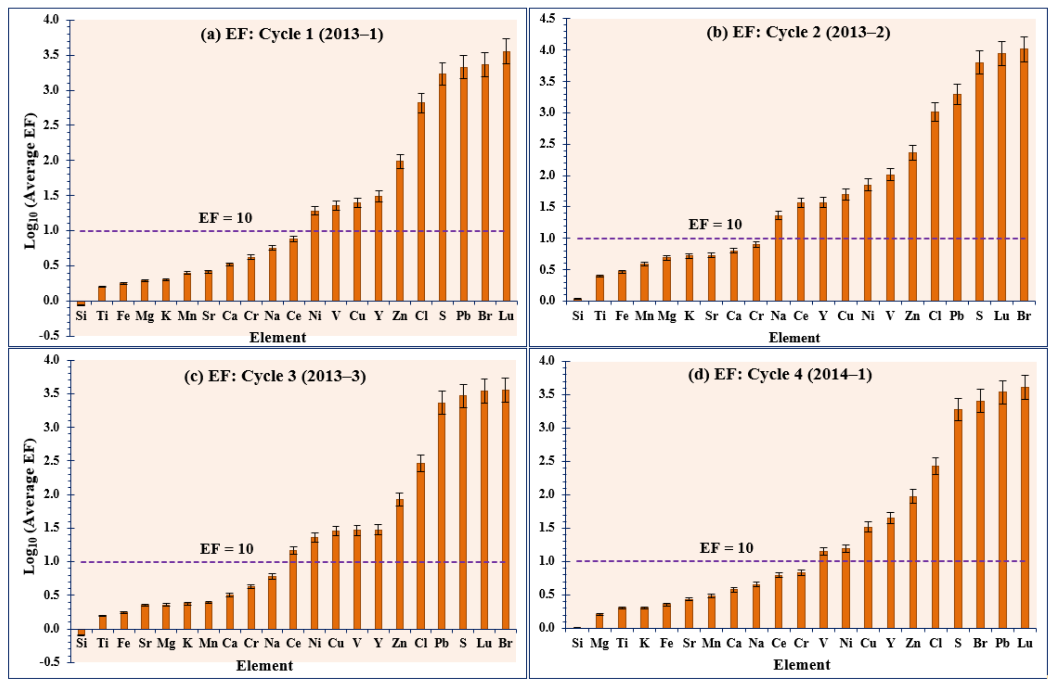
3.5. Elemental Enrichment Factor (EF)

The distribution of natural and anthropogenic TEs per cycle is presented in Figure 5 and Supplemental Materials (Table S5). Anthropogenic sources as indicated by EF > 10, contributed significantly to Ni, V, Cu, Y, Zn, Cl, S, Pb, Br, and Lu; while the earth-crust derived TEs (EF ≤ 10) included Si, Ti, Fe, Mg, K, Mn, Sr, Ca, Cr, Na, Ce, and Al. Whereas a TE may be classified as earth-crust derived based on the EF value, it is important to note that there could be some proportions coming from the anthropogenic sources. Notably, EF, when combined with other analyses such as PMF, principal component analysis, and chemical mass balance, can be key to defining the overall extent of anthropogenic influence in air pollution research.
Apart from sulfur (S), anthropogenic TEs contributed a small portion (~1.6%) of the overall PM2.5. Though Cl was classified as anthropogenic by EF, Cl is typically associated with marine input as sea-sprays. With Jeddah’s location, the contribution of sea-sprays during the study was likely substantial. Vanadium (V) and S are typically associated with oil combustion processes as seen in petrol-chemical industries. V occurs naturally in fossil-fuels, natural oil deposits, and in about 65 different minerals [73], while S is typically emitted as SO2 from fossil-fuel/oil combustion processes. Copper (Cu), Zn, Ni, Br, and Pb can originate from vehicular emissions [73,74] and several industrial processes (especially Ni and Br). Notably, Cu and Zn have antioxidant properties that attract their use in engine oil. Notably, though Saudi Arabia phased out the use of leaded gasoline in January 2001, as of 2011, the allowable Pb content in gasoline remained at 13 mg/L, which meant that in high traffic density cities the EF of Pb would still be elevated. It was estimated that total Pb in consumed fuel in Jeddah was about 83.6 tons per year [3,74]. Over the years, with continued implementation of the ban on Pb-gasoline, the current Pb emissions from automobiles are considerably lower. However, the environmental Pb contamination is still an issue and may be attributable to several sources. In addition, the ban on Pb-gasoline implied the phasing out of the use of Br as an essential component of engine anti-knock fluid. However, Br compounds are still being used in batteries of electric cars designed to produce zero BC and NOX emissions, and several other applications (such as, water treatment, pesticides, and drugs).
Rare earth TEs (Lu, Ce, and Y) were also quantified above their respective limits of quantification (LOQs). Being rare, these elements in PM2.5 are typically indicative of anthropogenic applications. For example, the stable isotopes of Lu (175Lu and 176Lu) are used as catalysts in petroleum industry for cracking hydrocarbons in oil refineries [1,75], while Ce is used as a fuel additive to cut automobile emissions. The oxides of Ce are also used to catalyze petroleum cracking in petroleum refineries (CeO) [76,77], and as a catalytic converter in automobiles (Ce2O3), for oxidation of CO and NOX emissions [78].

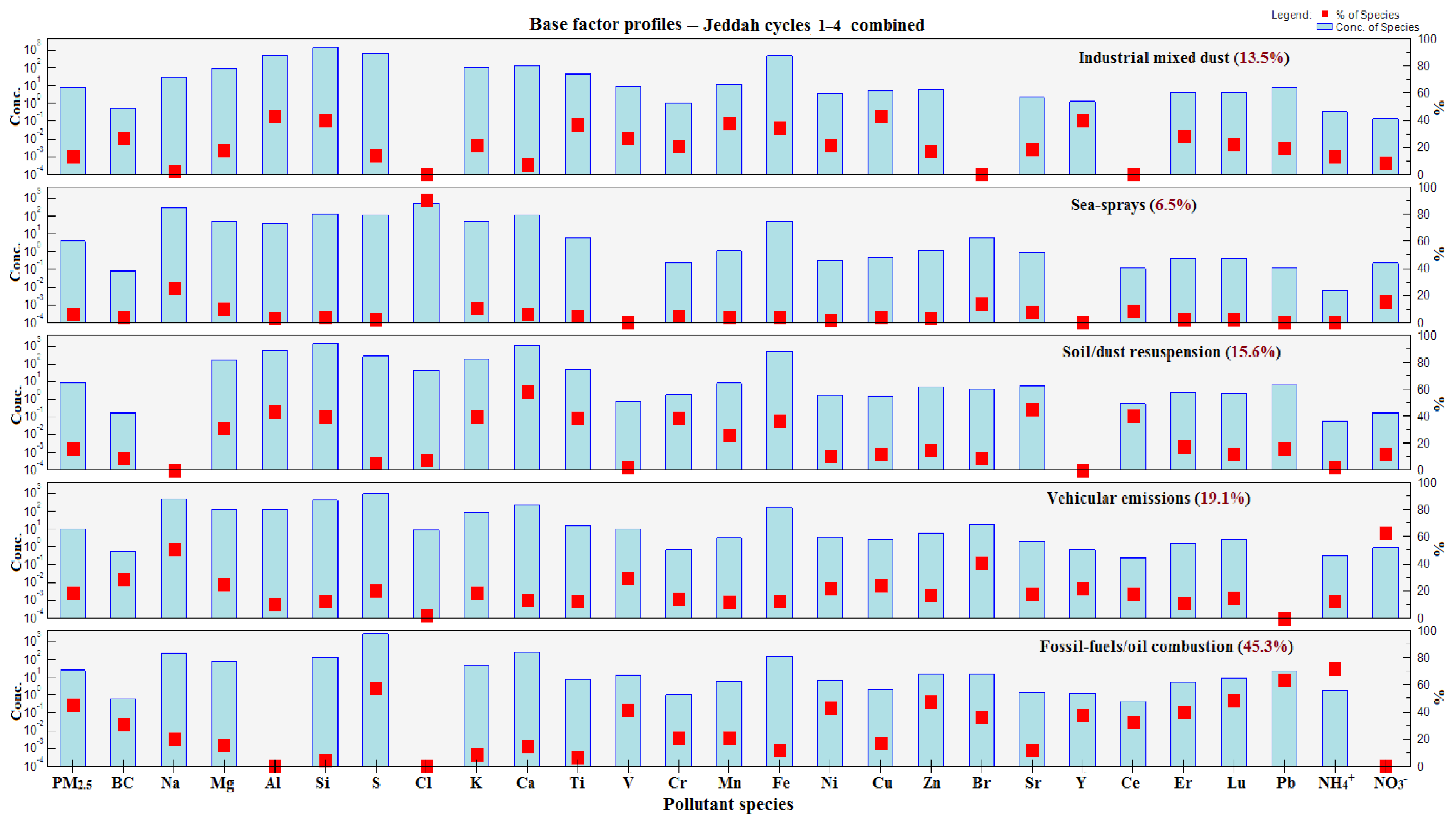
3.6. Positive Matrix Factorization (PMF)

PMF (version 5.0.14) was applied to resolve the emission sources of PM2.5 in Jeddah. To improve the study statistical power, we performed the PMF analysis utilizing data from combined cycles. The results are presented in Table 2 and Figure 6 and Figure S3. Due to substantial seasonal variations in pollutant concentrations, we performed additional analyses per cycle, to evaluate seasonal variations in emission sources. Results are presented in Supplemental Materials (Tables S6 and S7 and Figures S4–S7). Sulfur (S) and SO42 are basically related since SO42 is formed as a secondary aerosol from oxidation of SO2. However, S from ED–XRF represents the total S, while SO42 represents only the water–soluble portion of S. Since there were significant over– and under–estimates in SO42 per cycle (Table S3), total S from ED–XRF became more favorable for the PMF analysis. Moreover, though S and SO42 were highly correlated (R2 = 0.79–0.98), these correlations varied significantly by cycle (Figure S8), making S a better option for the PMF analysis. Oxalate (C2O42) was excluded from PMF analysis due to its low levels in all the samples.
A rotational tool (bootstrap analysis) was used to estimate the factor-related uncertainties and assess the rotational uncertainty of our PMF models. We compared the factors between each bootstrap run with the initial PMF output. The PMF solutions that did not attain optimal factor separation (as shown by the residual analyses) were not considered for further analyses. We then used the retained solutions to further test the robustness of our PMF models output(s). Finally, we resolved the PMF base models at 20 runs with five (5) factors. As a quality control and robustness test, we ran/applied the selected base models 5–10 times each, to test the consistency of the results (PMF outputs). Typically, PMF outputs are always consistent and attain a 100% convergence on all the runs when the PMF models are resolved with the correct number of factors.
Overall, the Q-values (Q-robust and Q-true) for all the models were consistent and within a close range, following multiple runs. Given that the Q-robust values are based on the model with controlled outliers, while the Q-true values include outliers, the observed slight differences in the Q-values implied a perfect fit for the data within each model. Additionally, all the models attained a 100% convergence rate on all the runs, and thus alluding more to the accuracy of the number of factors used. The presented PMF results are based on the run with the lowest Q-robust value. However, given the minor differences in the Q-values, results were similar for all the runs.
From the diagnostics data (residual analyses), most of the pollutant species had normally distributed residuals and relatively high signal-to-noise ratios (S/N), except Ce (Table 2). Thus, Ce was classified as “weak”, to limit its influence on the results. Additionally, since we were delineating the PM2.5 emission sources, PM2.5 as a parameter was categorized as “weak” to restrict it from strongly influencing the model results. Pollutant species with S/N > 5 were all classified as “strong” (Table 2 and Table S7).
The interpretation of factors to determine the PM2.5 emission sources was done by comparing the factor loadings in the profiles of each pollutant specie, as presented in Figure 6 and Figure S3. The chemical components of PM2.5 originate from specific sources as discussed in previous sections, and thus can be used as markers for source identification.
Overall, the five delineated PM2.5 sources in Jeddah were: (1) fossil-fuels/oil combustion (45.3%)—S, V, Pb, Ni, Lu, Zn, Br, Y, and BC; (2) vehicular emissions (19.1%)—NO3, Br, Cu, Zn, Ni, V, S, Mg, Na, and BC; (3) soil/dust resuspension (15.6%)—Mg, Al, Si, K, Ca, Ti, Cr, Mn, Fe, Zn, Sr, Er and Pb; (4) industrial mixed dust (13.5%)—Mg, Al, Si, S, K, Ti, V, Cr, Mn, Fe, Ni, Cu, Zn, Sr, Y, Er, Lu, Pb and BC. Jeddah has several industries and heavy vehicular traffic. The industrial dust contained a mixture of pollutants emitted from several anthropogenic activities; and (5) sea-spray (6.5%)—Cl, Na, Mg, K, and Ca. Jeddah’s location at the coast of the Red Sea, makes the contribution from sea-sprays to the overall air pollution significant.

3.7. Backward-In-Time Trajectories

Plots of wind trajectories 72 h prior to sampling for the two days with the highest and lowest PM2.5 levels per cycle are presented under Supplemental Materials (Figures S9–S12). The days with wind flowing over the Red Sea into Jeddah had the lowest PM2.5. Ideally, the air above the sea has lower PM levels, which introduces a dilution effect. Conversely, wind flowing over inland areas into Jeddah had higher PM2.5. Jeddah and the neighboring cities of Makkah, Medina, and Rabigh are heavily industrialized. This presented an opportunity to pick up pollutants from these neighboring cities into Jeddah. This also further highlights the significance of local and regional emissions to the PM2.5 levels in Jeddah.
Notably, during cycle 4 (Figure S12), one of the days with high PM2.5 (27 January 2014) had wind trajectories passing over the Red Sea. On this day, the southeasterly gusty winds originating from the Gulf of Eden were associated with a dust-storm event from 12:00 pm to 19:00 pm which contributed to the high PM2.5 levels observed on that day.
Overall, across the study period, the wind trajectories indicated that local and regional emissions, as well as the long-distance transport, may have contributed significantly to the observed PM2.5.

4. Conclusions

This is a comprehensive assessment of PM2.5 air pollution, providing a thorough delineation of the major emission sources in Jeddah. The observed PM2.5 levels exceeded the WHO (15 μg/m3) and Saudi Arabia’s PME (35 μg/m3) guidelines, stressing a major pollution issue. Results highlight a significant anthropogenic influence on air pollution levels in Jeddah and thus, will be key to refining the local policies on air pollution. From delta–C estimates, results indicated little to no PM2.5 emissions from biomass combustion. Conversely, the estimates of p-SO42, p-NO3, and p-NH4+ were significantly high, indicating major PM2.5 emissions from industrial and automobile sources. Furthermore, EF defined several anthropogenic TEs (Ni, V, Cu, Zn, Pb, S, Lu, and Br) that were intricately linked to industrial and automobile emissions. Further analyses from PMF resolved five (5) major sources including: fossil-fuels/oil combustion (45.3%), vehicular emissions (19.1%), soil/dust resuspension (15.6%), industrial mixed dust (13.5%) and sea-spray (6.5%).
Anthropogenic sources contributed ~78% of the measured PM2.5 with the largest proportions coming from industrial and vehicular emissions. Thus, future policies on particulate air pollution may need to target these two sources. Furthermore, given the existing body of evidence of adverse health outcomes at much lower exposure levels than reported in this study, the current PME guideline on PM2.5 needs to be revised to lower the acceptable levels as well as enforce strict compliance. Introduction of go-green policies in mass transit systems may be a great idea. Go-green policies may involve the electrification and hybridization of the existing transport modes, to reduce the overdependency on petroleum, and thus lower the BC and NOX emissions.
Notably, the wind trajectories highlighted a possible major pollution contribution from regional and long-distance transport. Thus, a regional approach to air pollution control will be more beneficial and effective, given the long-distance transport. In addition, as per the suggestion from the reviewers, future studies utilizing wind trajectories may need to incorporate additional receptor analyses based on hybrid receptor models (such as the potential source contribution function (PSCF) model, CWT, etc.) to analyze the spatial distribution and ultimately quantify the contribution from regional/long-distance transport. These models are applicable on both the PM2.5 and PMF reconstructed sources that are potentially influenced by wind transport. This is a key feature for further assessment of the potential contribution of long-distance transport to the observed PM2.5 levels.
Overall, our results supplement the previously published data, and further highlight the need for more research to fully appreciate the major air pollution related issues in Saudi Arabia. This is key to both the formulation and enactment of sustainable policies on air pollution for the entire Middle East region.

Supplementary Materials

The following supporting information can be downloaded at: https://www.mdpi.com/article/10.3390/atmos13050711/s1, Figure S1: An assembled PM2.5 sampler showing the major components—Photo by author(s); Figure S2: Comparison of mean PM2.5 levels measured in Jeddah with other cities worldwide; Figure S3: Factor fingerprints and contributions to the overall PM2.5 in Jeddah—combined cycles; Figure S4: Base factor profiles and contributions to the overall PM2.5—Jeddah cycle 1; Figure S5: Base factor profiles and contributions to the overall PM2.5—Jeddah cycle 2; Figure S6: Base factor profiles and contributions to the overall PM2.5—Jeddah cycle 3; Figure S7: Base factor profiles and contributions to the overall PM2.5—Jeddah cycle 4; Figure S8: Plots of water-soluble SO42− from IC analysis versus total S from ED-XRF analysis; Figure S9: Plots of backward-in-time wind trajectories showing wind direction and its influence on daily PM2.5 measured in Jeddah (cycle 1); Figure S10: Plots of backward-in-time wind trajectories showing wind direction and its influence on daily PM2.5 measured in Jeddah (cycle 2); Figure S11: Plots of backward-in-time wind trajectories showing wind direction and its influence on daily PM2.5 measured in Jeddah (cycle 3); Figure S12: Plots of backward-in-time wind trajectories showing wind direction and its influence on daily PM2.5 measured in Jeddah (cycle 4); Table S1: Summary of the optimum conditions for analysis of water-soluble cations and anions by ion exchange chromatography; Table S2: Typical detection limits of elements measured on a Thermo Scientific™ ARL™ QUANT’X ED-XRF Spectrometer; Table S3: Summary of the overall variations in expected and observed SO42−, NH4+ and NO3 during the four sampling cycles in Jeddah, Saudi Arabia; Table S4: Pearson correlations between different pollutant species measured from PM2.5 and with meteorology; Table S5: Mean values for the elemental enrichment factors (EFs) per study cycle; Table S6: Summary of the PMF solution in Jeddah: Sources of PM2.5 and their overall relative contributions; Table S7: Signal-to-Noise ratios (S/N) and classifications/categories of air pollutant species used for PMF analysis per cycle in Jeddah.

Author Contributions

Data analysis and organization, interpretation of data, writing original draft, S.R.N.; project administration, funding, review of data, O.S.A.; field measurements, data review, A.S.; experimental execution, M.M.H.; field measurements, J.Z.; software, F.K.; data review and editing, D.O.C.; data review and editing, D.R.B.; conceptualization, supervision, methodology, review, and editing, H.A.K. All authors have read and agreed to the published version of the manuscript.

Funding

This work was supported by a grant from King Abdul-Aziz University, Jeddah, Saudi Arabia.

Institutional Review Board Statement

Not applicable.

Informed Consent Statement

Not applicable.

Data Availability Statement

Not applicable.

Acknowledgments

This research was supported by a grant from King Abdul-Aziz University, Jeddah, Saudi Arabia. The authors are also grateful to Dr. Lung C. Chen, of New York University, School of Medicine, for his support analyzing trace elements by ED-XRF. The authors would also like to acknowledge the contribution of peer reviewer(s) that significantly improved the quality of this publication.

Conflicts of Interest

The authors declare no conflict of interest.

References

  1. Nayebare, S.R.; Aburizaiza, O.S.; Khwaja, H.A.; Siddique, A.; Hussain, M.M.; Zeb, J.; Khatib, F.; Carpenter, D.O.; Blake, D.R. Chemical Characterization and Source Apportionment of PM2.5 in Rabigh, Saudi Arabia. Aerosol Air Qual. Res. 2016, 16, 3114–3129. [Google Scholar] [CrossRef] [Green Version]
  2. Alharbi, B.; Shareef, M.M.; Husain, T. Study of chemical characteristics of particulate matter concentrations in Riyadh, Saudi Arabia. Atmos. Pollut. Res. 2015, 6, 88–98. [Google Scholar] [CrossRef] [Green Version]
  3. Khodeir, M.; Shamy, M.; Alghamdi, M.; Zhong, M.; Sun, H.; Costa, M.; Chen, L.-C.; Maciejczyk, P. Source Apportionment and Elemental Composition of PM2.5 and PM10 in Jeddah City, Saudi Arabia. Atmos. Pollut. Res. 2012, 3, 331–340. [Google Scholar] [CrossRef] [PubMed] [Green Version]
  4. Munir, S.; Habeebullah, T.M.; Seroji, A.R.; Gabr, S.S.; Mohammed, A.M.F.; Morsy, E.A. Modeling Particulate Matter Concentrations in Makkah, Applying a Statistical Modeling Approach. Aerosol Air Qual. Res. 2013, 13, 901–910. [Google Scholar] [CrossRef] [Green Version]
  5. WHO. The World Health Organization (WHO) Air Quality Guidelines-Global Update 2021: Ambient (Outdoor) Air Quality and Health. 2021. Available online: https://www.who.int/news-room/fact-sheets/detail/ambient-(outdoor)-air-quality-and-health (accessed on 29 March 2022).
  6. PME. Presidency of Meteorology and Environment (PME), Ambient Air Quality Standards. Available online: http://www.pme.gov.sa/en/En_EnvStand19.pdf (accessed on 12 April 2016).
  7. Nayebare, S.R. Fine Particulate Air Pollution in Saudi Arabia–Implications for Cardiopulmonary Morbidity; State University of New York: Albany, NY, USA, 2016. [Google Scholar]
  8. Nasrallah, M.M.; Seroji, A.R. Particulates in the Atmosphere of Makkah and Mina Valley during Ramadhan and Hajj Season of 1424 and 1425 H (2004–2005). Arab Gulf J. Sci. Res. 2008, 26, 199–206. [Google Scholar]
  9. Khreis, H.; Cirach, M.; Mueller, N.; Hoogh, K.D.; Hoek, G.; Nieuwenhuijsen, M.J.; Rojas-Rueda, D. Outdoor air pollution and the burden of childhood asthma across Europe. Eur. Respir. J. 2019, 54, 1802194. [Google Scholar] [CrossRef]
  10. Guerreiro, C.B.B.; Foltescu, V.; De Leeuw, F. Air quality status and trends in Europe. Atmos. Environ. 2014, 98, 376–384. [Google Scholar] [CrossRef] [Green Version]
  11. Sillanpää, M.; Frey, A.; Hillamo, R.; Pennanen, A.S.; Salonen, R.O. Organic, elemental and inorganic carbon in particulate matter of six urban environments in Europe. Atmos. Chem. Phys. 2005, 5, 2869–2879. [Google Scholar] [CrossRef] [Green Version]
  12. Anderson, H.; Bremner, S.; Atkinson, R.; Harrison, R.; Walters, S. Particulate matter and daily mortality and hospital admissions in the west midlands conurbation of the United Kingdom: Associations with fine and coarse particles, black smoke and sulphate. Occup. Environ. Med. 2001, 58, 504–510. [Google Scholar] [CrossRef] [Green Version]
  13. Sheffield, P.E.; Speranza, R.; Chiu, Y.-H.M.; Hsu, H.-H.L.; Curtin, P.C.; Renzetti, S.; Pajak, A.; Coull, B.; Schwartz, J.; Kloog, I.; et al. Association between particulate air pollution exposure during pregnancy and postpartum maternal psychological functioning. PLoS ONE 2018, 13, e0195267. [Google Scholar] [CrossRef] [Green Version]
  14. Crouse, D.L.; Peters, P.A.; Van Donkelaar, A.; Goldberg, M.S.; Villeneuve, P.J.; Brion, O.; Khan, S.; Atari, D.O.; Jerrett, M.; Pope, C.A.; et al. Risk of Nonaccidental and Cardiovascular Mortality in Relation to Long-term Exposure to Low Concentrations of Fine Particulate Matter: A Canadian National-Level Cohort Study. Environ. Health Perspect. 2012, 120, 708–714. [Google Scholar] [CrossRef] [PubMed]
  15. Weuve, J.; Puett, R.C.; Schwartz, J.; Yanosky, J.D.; Laden, F.; Grodstein, F. Exposure to Particulate Air Pollution and Cognitive Decline in Older Women. Arch. Intern. Med. 2012, 172, 219–227. [Google Scholar] [CrossRef] [PubMed] [Green Version]
  16. Bell, M.L.; Dominici, F.; Ebisu, K.; Zeger, S.L.; Samet, J.M. Spatial and Temporal Variation in PM2.5 Chemical Composition in the United States for Health Effects Studies. Environ. Health Perspect. 2007, 115, 989–995. [Google Scholar] [CrossRef] [PubMed] [Green Version]
  17. Pope, C.A.; Turner, M.C.; Burnett, R.T.; Jerrett, M.; Gapstur, S.M.; Diver, W.R.; Krewski, D.; Brook, R.D. Relationships between fine particulate air pollution, cardiometabolic disorders, and cardiovascular mortality. Circ. Res. 2015, 116, 108–115. [Google Scholar] [CrossRef] [PubMed]
  18. Brook, R.; Rajagopalan, S.; Pope, C.; Brook, J.; Bhatnagar, A.; Diez-Roux, A.; Holguin, F.; Hong, Y.; Luepker, R.; Mittleman, M.; et al. Particulate matter air pollution and cardiovascular disease: An update to the scientific statement from the American Heart Association. Circulation 2010, 121, 2331–2378. [Google Scholar] [CrossRef] [Green Version]
  19. Pope, C.A.I.; Dockery, D.W. Health Effects of Fine Particulate Air Pollution: Lines that Connect. J. Air Waste Manag. Assoc. 2006, 56, 709–742. [Google Scholar] [CrossRef]
  20. Pope, C.A.; Burnett, R.T.; Thurston, G.D.; Thun, M.J.; Calle, E.E.; Krewski, D.; Godleski, J.J. Cardiovascular Mortality and Long-Term Exposure to Particulate Air Pollution: Epidemiological Evidence of General Pathophysiological Pathways of Disease. Circulation 2004, 109, 71–77. [Google Scholar] [CrossRef] [Green Version]
  21. Peden, D.B. The epidemiology and genetics of asthma risk associated with air pollution. J. Allergy Clin. Immunol. 2005, 115, 213–219. [Google Scholar] [CrossRef]
  22. Sunyer, J.; Schwartz, J.; Tobías, A.; Macfarlane, D.; Garcia, J.; Antó, J.M. Patients with Chronic Obstructive Pulmonary Disease Are at Increased Risk of Death Associated with Urban Particle Air Pollution: A Case-Crossover Analysis. Am. J. Epidemiol. 2000, 151, 50–56. [Google Scholar] [CrossRef] [Green Version]
  23. SADP. Saudi Arabia Demographic Profile 2014; PopulationPyramid.Net: Saudi Arabia, 2014. [Google Scholar]
  24. Hasanean, H.; Almazroui, M. Rainfall: Features and Variations over Saudi Arabia, A Review. Climate 2015, 3, 578. [Google Scholar] [CrossRef] [Green Version]
  25. Ahmed, T.; Dutkiewicz, V.A.; Shareef, A.; Tuncel, G.; Tuncel, S.; Husain, L. Measurement of black carbon (BC) by an optical method and a thermal-optical method: Intercomparison for four sites. Atmos. Environ. 2009, 43, 6305–6311. [Google Scholar] [CrossRef]
  26. Rattigan, O.V.; Civerolo, K.; Doraiswamy, P.; Felton, H.D.; Hopke, P.K. Long term black carbon measurements at two urban locations in New York. Aerosol Air Qual. Res. 2013, 13, 1181–1196. [Google Scholar] [CrossRef] [Green Version]
  27. Wang, Y.; Hopke, P.K.; Rattigan, O.V.; Chalupa, D.C.; Utell, M.J. Multiple-year black carbon measurements and source apportionment using Delta-C in Rochester, New York. J. Air Waste Manag. Assoc. 2012, 62, 880–887. [Google Scholar] [CrossRef] [PubMed] [Green Version]
  28. Shaltout, A.A.; Boman, J.; Al-Malawi, D.A.R.; Shehadeh, Z.F. Elemental Composition of PM2.5 Particles Sampled in Industrial and Residential Areas of Taif, Saudi Arabia. Aerosol Air Qual. Res. 2013, 13, 1356–1364. [Google Scholar] [CrossRef] [Green Version]
  29. Yatkin, S.; Gerboles, M.; Borowiak, A. Evaluation of standardless EDXRF analysis for the determination of elements on PM10 loaded filters. Atmos. Environ. 2012, 54, 568–582. [Google Scholar] [CrossRef]
  30. Xu, H.M.; Cao, J.J.; Ho, K.F.; Ding, H.; Han, Y.M.; Wang, G.H.; Chow, J.C.; Watson, J.G.; Khol, S.D.; Qiang, J.; et al. Lead concentrations in fine particulate matter after the phasing out of leaded gasoline in Xi’an, China. Atmos. Environ. 2012, 46, 217–224. [Google Scholar] [CrossRef]
  31. Korzhova, E.N.; Kuznetsova, O.V.; Smagunova, A.N.; Stavitskaya, M.V. Determination of inorganic pollutants in atmospheric aerosols. J. Anal. Chem. 2011, 66, 222–240. [Google Scholar] [CrossRef]
  32. Margui, E.; Van Grieken, R. X-Ray Fluorescence Spectrometry and Related Techniques; Momentum Press, LLC.: New York, NY, USA, 2013. [Google Scholar]
  33. Buhrke, V.E.; Jenkins, R.; Smith, D.K. Practical Guide for the Preparation of Specimens for X-ray Fluorescence and X-ray Diffraction Analysis; Wiley: Hoboken, NJ, USA, 1998. [Google Scholar]
  34. Thermo-Scientific. Analysis of Air Filters by ARL QUANT’X High Performance Energy Dispersive X-ray Fluorescence Spectrometer (EDXRF). 2007. Available online: https://www.thermofisher.com/document-connect/document-connect.html?url=https%3A%2F%2Fassets.thermofisher.com%2FTFS-Assets%2FMSD%2FApplication-Notes%2FXRAN41964-air-filter-analysis-EDXRF.pdf (accessed on 29 March 2022).
  35. Chow, J.C.; Lowenthal, D.; Chen, L.W.A.; Wang, X.; Watson, J. Mass reconstruction methods for PM2.5: A review. Air Qual. Atmos. Health 2015, 8, 243–263. [Google Scholar] [CrossRef] [Green Version]
  36. Watson, J.G.; Chow, J.C.; Lowenthal, D.H.; Chen, L.-W.A.; Wang, X.; Biscay, P. Reformulation of PM2.5 Mass Reconstruction Assumptions for the San Joaquin Valley Final Report; Desert Research Institute, Nevada System of Higher Education: Reno, NV, USA, 2012. [Google Scholar]
  37. Macias, E.S.; Zwicker, J.O.; Ouimette, J.R.; Hering, S.V.; Friedlander, S.K.; Cahill, T.A.; Kuhlmey, G.A.; Richards, L.W. Regional haze case studies in the southwestern US—I. Aerosol chemical composition. Atmos. Environ. (1967) 1981, 15, 1971–1986. [Google Scholar] [CrossRef]
  38. Solomon, P.A.; Fall, T.; Salmon, L.; Cass, G.R.; Gray, H.A.; Davidson, A. Chemical characteristics of PM10 aerosols collected in the Los Angeles area. JAPCA 1989, 39, 154–163. [Google Scholar] [CrossRef]
  39. Seinfeld, J.H.; Pandis, S.N. Atmospheric Chemistry and Physics: From Air Pollution to Climate Change; John Wiley & Sons: Hoboken, NJ, USA, 2012. [Google Scholar]
  40. Fabretti, J.-F.; Sauret, N.; Gal, J.-F.; Maria, P.-C.; Schärer, U. Elemental characterization and source identification of PM2.5 using Positive Matrix Factorization: The Malraux road tunnel, Nice, France. Atmos. Res. 2009, 94, 320–329. [Google Scholar] [CrossRef]
  41. Sofowote, U.M.; McCarry, B.E.; Marvin, C.H. Source Apportionment of PAH in Hamilton Harbour Suspended Sediments: Comparison of Two Factor Analysis Methods. Environ. Sci. Technol. 2008, 42, 6007–6014. [Google Scholar] [CrossRef] [PubMed]
  42. Hopke, P.K. A Guide to Positive Matrix Factorization (PMF); Center for Air Resources Engineering and Science, Clarkson University: Potsdam, NY, USA, 2000; pp. 1–16. [Google Scholar]
  43. Vivone, G.; D’Amico, G.; Summa, D.; Lolli, S.; Amodeo, A.; Bortoli, D.; Pappalardo, G. Atmospheric Boundary Layer height estimation from aerosol lidar: A new approach based on morphological image processing techniques-(Preprint). Atmos. Chem. Phys. 2020, 21, 4249–4265. [Google Scholar] [CrossRef]
  44. Ramana, M.V.; Krishnan, P.; Nair, S.M.; Kunhikrishnan, P.K. Thermodynamic structure of the Atmospheric Boundary Layer over the Arabian Sea and the Indian Ocean during pre-INDOEX and INDOEX-FFP campaigns. Ann. Geophys. 2004, 22, 2679–2691. [Google Scholar] [CrossRef] [Green Version]
  45. Li, W. Study of Diurnal Cycle Variability of Planetary Boundary Layer Characteristics over the Red Sea and Arabian Peninsula; King Abdullah University of Science and Technology (KAUST): Thuwal, Saudi Arabia, 2012. [Google Scholar] [CrossRef]
  46. Draxler, R.R.; Rolph, G.D. HYSPLIT (HYbrid Single-Particle Lagrangian Integrated Trajectory) Model Access via NOAA ARL READY Website. NOAA Air Resources Laboratory, College Park, MD. Available online: http://www.arl.noaa.gov/HYSPLIT.php (accessed on 13 July 2021).
  47. Rolph, G.D. Real-Time Environmental Applications and Display sYstem (READY) Website. NOAA Air Resources Laboratory, College Park, MD. Available online: http://www.ready.noaa.gov (accessed on 13 July 2021).
  48. Jish Prakash, P.; Stenchikov, G.; Kalenderski, S.; Osipov, S.; Bangalath, H. The impact of dust storms on the Arabian Peninsula and the Red Sea. Atmos. Chem. Phys. 2015, 15, 199–222. [Google Scholar] [CrossRef] [Green Version]
  49. Singh, N.; Murari, V.; Kumar, M.; Barman, S.C.; Banerjee, T. Fine particulates over South Asia: Review and meta-analysis of PM2.5 source apportionment through receptor model. Environ. Pollut. 2017, 223, 121–136. [Google Scholar] [CrossRef] [PubMed]
  50. Jennifer, G.; Paul, K. Preliminary Examination of Trace Elements in Tyres, Brake Pads and Road Bitumen in New Zealand; Ministry of Transport: Wellington, New Zealand, 2003.
  51. U.S.EPA. The National Ambient Air Quality Standards for Particle Pollution. Revised Air Quality Standards for Particle Pollution and Updates to the Air Quality Index (AQI); U.S.EPA: Washington, DC, USA, 2012.
  52. Zhao, X.; Zhang, X.; Xu, X.; Xu, J.; Meng, W.; Pu, W. Seasonal and diurnal variations of ambient PM2.5 concentration in urban and rural environments in Beijing. Atmos. Environ. 2009, 43, 2893–2900. [Google Scholar] [CrossRef]
  53. Begum, B.A.; Hossain, A.; Nahar, N.; Markwitz, A.; Hopke, P.K. Organic and black carbon in PM2.5 at an urban site at Dhaka, Bangladesh. Aerosol Air Qual. Res. 2012, 12, 1062–1072. [Google Scholar] [CrossRef] [Green Version]
  54. Amarsaikhan, D.; Battsengel, V.; Nergui, B.; Ganzorig, M.; Bolor, G. A Study on Air Pollution in Ulaanbaatar City, Mongolia. J. Geosci. Env. Prot. 2014, 2, 123. [Google Scholar] [CrossRef]
  55. Kulshrestha, A.; Satsangi, P.G.; Masih, J.; Taneja, A. Metal concentration of PM2.5 and PM10 particles and seasonal variations in urban and rural environment of Agra, India. Sci. Total Environ. 2009, 407, 6196–6204. [Google Scholar] [CrossRef] [PubMed]
  56. Hamad, S.H.; Schauer, J.J.; Heo, J.; Kadhim, A.K.H. Source apportionment of PM2.5 carbonaceous aerosol in Baghdad, Iraq. Atmos. Res. 2015, 156, 80–90. [Google Scholar] [CrossRef]
  57. Yatkin, S.; Bayram, A. Source apportionment of PM10 and PM2.5 using positive matrix factorization and chemical mass balance in Izmir, Turkey. Sci. Total Environ. 2008, 390, 109–123. [Google Scholar] [CrossRef] [PubMed]
  58. Kermani, M.; Arfaeinia, H.; Nabizadeh, R.; Alimohammadi, M.; Aalamolhoda, A. Levels of PM2.5—associated heavy metals in the ambient air of Sina hospital district, Tehran, Iran. J. Air Pollut. Health 2015, 1, 1–6. [Google Scholar]
  59. Brown, K.W.; Bouhamra, W.; Lamoureux, D.P.; Evans, J.S.; Koutrakis, P. Characterization of Particulate Matter for Three Sites in Kuwait. J. Air Waste Manag. Assoc. 2008, 58, 994–1003. [Google Scholar] [CrossRef]
  60. Degobbi, C.; Lopes, F.D.; Carvalho-Oliveira, R.; Muñoz, J.E.; Saldiva, P.H. Correlation of fungi and endotoxin with PM2.5 and meteorological parameters in atmosphere of Sao Paulo, Brazil. Atmos. Environ. 2010, 45, 2277–2283. [Google Scholar] [CrossRef]
  61. Akyuz, M.; Cabuk, H. Meteorological variations of PM2.5/PM10 concentrations and particle-associated polycyclic aromatic hydrocarbons in the atmospheric environment of Zonguldak, Turkey. J. Hazard Mater. 2009, 170, 13–21. [Google Scholar] [CrossRef]
  62. Nakhle, M.M.; Farah, W.; Ziade, N.; Abboud, M.; Coussa-Koniski, M.L.; Annesi-Maesano, I. Beirut Air Pollution and Health Effects—BAPHE study protocol and objectives. Multidiscip. Respir. Med. 2015, 10, 21. [Google Scholar] [CrossRef] [Green Version]
  63. Hueglin, C.; Gehrig, R.; Baltensperger, U.; Gysel, M.; Monn, C.; Vonmont, H. Chemical characterization of PM2.5, PM10 and coarse particles at urban, near-city and rural sites in Switzerland. Atmos. Environ. 2005, 39, 637–651. [Google Scholar] [CrossRef]
  64. Pateraki, S.; Assimakopoulos, V.; Maggos, T.; Fameli, K.; Kotroni, V.; Vasilakos, C. Particulate matter pollution over a Mediterranean urban area. Sci. Total Environ. 2013, 463–464, 508–524. [Google Scholar] [CrossRef]
  65. Khan, M.F.; Shirasuna, Y.; Hirano, K.; Masunaga, S. Characterization of PM2.5, PM2.5–10 and PM10 in ambient air, Yokohama, Japan. Atmos. Res. 2010, 96, 159–172. [Google Scholar] [CrossRef]
  66. Zhuang, H.; Chan, C.K.; Fang, M.; Wexler, A.S. Formation of nitrate and non-sea-salt sulfate on coarse particles. Atmos. Environ. 1999, 33, 4223–4233. [Google Scholar] [CrossRef]
  67. Zhuang, H.; Chan, C.K.; Fang, M.; Wexler, A.S. Size distributions of particulate sulfate, nitrate, and ammonium at a coastal site in Hong Kong. Atmos. Environ. 1999, 33, 843–853. [Google Scholar] [CrossRef]
  68. Wioletta, R.-K.; Izabela, S.; Barbara, M.; Krzysztof, K.; Anna, Z.; Kornelia, K. Size-Resolved Water-Soluble Ionic Composition of Ambient Particles in an Urban Area in Southern Poland. J. Environ. Prot. 2013, 4, 371–379. [Google Scholar] [CrossRef] [Green Version]
  69. Bauer, S.E.; Koch, D.; Unger, N.; Metzger, S.M.; Shindell, D.T.; Streets, D.G. Nitrate aerosols today and in 2030: A global simulation including aerosols and tropospheric ozone. Atmos. Chem. Phys. 2007, 7, 5043–5059. [Google Scholar] [CrossRef] [Green Version]
  70. U.S.EPA. Atmospheric Ammonia: Sources and Fate: A Review of Ongoing Federal Research and Future Needs; U.S.EPA: Washington, DC, USA, 2000.
  71. Frank, N.H. Retained nitrate, hydrated sulfates, and carbonaceous mass in federal reference method fine particulate matter for six eastern U.S. cities. J. Air Waste Manag. Assoc. 2006, 56, 500–511. [Google Scholar] [CrossRef] [PubMed]
  72. Chow, J.C.; Watson, J.G.; Lowenthal, D.H.; Magliano, K.L. Loss of PM2.5 nitrate from filter samples in central California. J. Air Waste Manag. Assoc. 2005, 55, 1158–1168. [Google Scholar] [CrossRef] [PubMed] [Green Version]
  73. Raask, E. The mode of occurrence and concentration of trace elements in coal. Prog. Energy Combust. Sci. 1985, 11, 97–118. [Google Scholar] [CrossRef]
  74. Aburas, H.M.; Zytoon, M.A.; Abdulsalam, M.I. Atmospheric Lead in PM2.5 after Leaded Gasoline Phase-out in Jeddah City, Saudi Arabia. Clean-Soil Air Water 2011, 39, 711–719. [Google Scholar] [CrossRef]
  75. RSC. Royal Society of Chemistry (RSC): Uses and Properties of Lutetium (Lu). Available online: http://www.rsc.org/periodic-table/element/71/lutetium (accessed on 6 June 2016).
  76. Steinbach, C. Cerium Dioxide (CeO2) - Overview. nanopartikel.info (2011-02-02). Available online: http://nanopartikel.info/en/nanoinfo/materials/cerium-dioxide (accessed on 6 June 2016).
  77. Trovarelli, A. Catalysis by Ceria and Related Materials; Imperial College Press: London, UK, 2002. [Google Scholar]
  78. Bleiwas, D.I. Potential for Recovery of Cerium Contained in Automotive Catalytic Converters: U.S. Department of the Interior; U.S. Geological Survey Open-File Report 2013–1037; U.S. Geological Survey: Reston, VA, USA, 2013; p. 10.
Figure 1. Map of Jeddah showing the sampling sites (King Abdul-Aziz Hospital (KAH), King Fahad Hospital (KFH), King Abdul-Aziz University (Al-Rehab/KAU)), industrial areas, major roads, and hospitals. Al-Rawda sampling site not depicted.
Atmosphere 13 00711 g001
Figure 2. Time-series plots for the 24-h PM2.5, BC, and meteorology during the study period in Jeddah—averaged sampling sites.
Atmosphere 13 00711 g002
Figure 3. Bar graphs showing the Air Quality Index for PM2.5 measured in Jeddah. AQI computations are based on the provisions of the United Sates Environmental Protection Agency (U.S. EPA).
Atmosphere 13 00711 g003
Figure 4. Variations in the observed and reconstructed PM2.5 per cycle averaged sampling sites: cycle 1—(a), cycle 2—(b), cycle 3—(c), cycle 4—(d) The relative proportions of daily PM2.5 explained by crustal material (CM), trace elements (TE), sea sprays (SS), secondary ions (SI), and black carbon (BC) per cycle are also provided.
Atmosphere 13 00711 g004
Figure 5. The log transformed enrichment factors (EFs) of trace elements measured from PM2.5 per cycle—averaged sampling sites: cycle 1—(a), cycle 2—(b), cycle 3—(c), cycle 4—(d). Elements with EF values exceeding 10 (as indicated by the dotted line), have significant proportions coming from anthropogenic emission sources.
Atmosphere 13 00711 g005
Figure 6. Base factor profiles and contributions to the overall PM2.5—all cycles combined.
Atmosphere 13 00711 g006
Table 1. Summarized 24-h PM2.5, BC, TEs, IS, and meteorology (mean daily temperature, relative humidity (RH) and wind speed (WS)) per sampling cycle in Jeddah.
Cycle 1Cycle 2Cycle 3Cycle 4
ParameterMean ± S.DMinMaxMean ± S.DMinMaxMean ± S.DMinMaxMean ± S.DMinMax
PM2.5 (μg/m3)58.8 ± 2522.311836.2 ± 12.321.38033.9 ± 9.118.56338 ± 17.712.490.8
BCIR (μg/m3)1.9 ± 0.60.82.91.8 ± 0.40.82.72.4 ± 0.61.44.02.3 ± 0.80.94.6
BCUV (μg/m3)1.6 ± 0.50.72.61.2 ± 0.30.61.81.6 ± 0.30.12.31.6 ± 0.50.73.3
Delta–C (μg/m3)−0.3 ± 0.2−0.90.1−0.6 ± 0.2−1.02−0.2−0.8 ± 0.3−1.7−0.3−0.6 ± 0.3−1.3−0.2
RH (%)53.6 ± 8.138.07156.2 ± 8.030.07163.8 ± 6.8477851.9 ± 122671.0
Temp. (°C)29.6 ± 2.624.434.427.2 ± 0.831.135.629.6 ± 1.227.831.725 ± 1.82027.8
WS (m/s)6.5 ± 2.13.0116.6 ± 1.54.0105.4 ± 1.63.0107.5 ± 3.03.015
Trace Elements, TEs (ng/m3)
Sulfur (S)4972 ± 2577132310,9354434 ± 1301127179736838 ± 2714262915,2244348 ± 221612149549
Silicon (Si)3427 ± 207672712,7332727 ± 378339716,4692255 ± 93157841973748 ± 273972314,151
Calcium (Ca)1780 ± 140466010,0151049 ± 56545527301216 ± 36762820371863 ± 13425007380
Iron (Fe)1367 ± 77235447601252 ± 16222837295945 ± 34031816651565 ± 11173475549
Aluminum (Al)1227 ± 83217751161052 ± 166253.17191830 ± 36115215681193 ± 98896.84812
Sodium (Na)1065 ± 51643429191151 ± 7211722552953 ± 4564802090735 ± 3882371723
Chlorine (Cl)547 ± 997DL5621261 ± 477DL1674108 ± 364DL2150219 ± 389DL1882
Magnesium (Mg)516 ± 2322271688397 ± 2341691181454 ± 121241767439 ± 3051081663
Potassium (K)490 ± 2872592160412 ± 2342081236412 ± 76.8286558460 ± 2921531622
Lead (Pb)318 ± 4012.73178389.2 ± 190DL1157294 ± 3044.711142361 ± 44116.12298
Titanium (Ti)126 ± 77.928.8498112 ± 1462562885.3 ± 3026.9152141 ± 9430.2458
Zinc (Zn)90.5 ± 14911.669660.9 ± 94.69.749452.1 ± 44.512.120653.3 ± 49.912.1224
Bromine (Br)50.2 ± 14.824.592.564 ± 22.921.211468.2 ± 18.436.513051.4 ± 20.325.7136
Vanadium (V)36.5 ± 19.8DL80.941.6 ± 14.222.174.732.8 ± 14.48.567.915.1 ± 13.1DL50.4
Manganese (Mn)31.3 ± 16.99.577.726.2 ± 32.43.414422.6 ± 8.76.141.535.3 ± 28.97.7148
Lutetium (Lu)21.4 ± 15.55.071.516.7 ± 11.46.256.615.8 ± 7.43.53518.5 ± 9.96.246
Nickel (Ni)17.3 ± 8.83.940.317.1 ± 5.79.037.115.0 ± 5.65.128.111.3 ± 6.22.831.4
Copper (Cu)17 ± 13.83.259.910.4 ± 5.83.626.213.6 ± 13.35.289.317.4 ± 12.93.670.5
Erbium (Er)16.1 ± 12.74.365.812.1 ± 123.955.810.9 ± 5.7DL28.214.6 ± 8.82.243.5
Strontium (Sr)12.2 ± 7.33.452.08.0 ± 5.12.825.97.6 ± 2.64.21412.9 ± 9.91.449.3
Yttrium (Y)11.3 ± 13DL58.35.0 ± 7.3DL39.610.2 ± 10.2DL37.312.2 ± 14.4DL75
Cerium (Ce)6.2 ± 5.8DL27.89.4 ± 7.9DL40.48.5 ± 3.9DL14.13.4 ± 3.0DL12.7
Chromium (Cr)5.2 ± 2.61.114.13.9 ± 3.71.119.13.6 ± 1.8DL9.36.4 ± 3.22.119.5
Water-soluble ions IS (μg/m3)
Sulfate (SO42−)17.8 ± 172.985.98.5 ± 3.21.922.912.1 ± 4.94.629.38.6 ± 4.72.120.2
Ammonium (NH4+)2.5 ± 1.90.28.32.4 ± 0.90.64.93.2 ± 1.31.26.53.2 ± 1.70.447.3
Nitrate (NO3)1.5 ± 0.90.14.11.1 ± 0.80.23.90.9 ± 0.60.12.31.2 ± 0.60.42.6
Oxalate (C2O42−)0.3 ± 0.1DL0.50.1 ± 0.10.040.20.1 ± 0.10.040.30.4 ± 0.50.021.9
Cycle 1 (Spring): 8 April–28 May 2013 (KAH, KFH and Al-Rawda—only the first 10 days were sampled at this site), Cycle 2 (Summer): 11 July–24 August 2013 (KAH and KFH), Cycle 3 (Fall): 2 October–16 November 2013 (KAH and Al-Rehab/or KAU), Cycle 4 (Winter): 7 January 2014–18 February 2014 (KAH and Al-Rehab/or KAU), DL: detection limit; S.D: standard deviation; BC: black carbon; TEs: trace elements/metals; IS: water-soluble ionic species.
Table 2. Signal-to-noise ratios (S/N), categories, and distribution of residuals for the pollutant species used for positive matrix factorization (PMF) analysis.
Pollutant SpeciesCategoryR2Normal ResidualsS/NModeled Samples (%)
PM2.5Weak0.39Yes10100
Black carbon (BC)Strong0.62Yes10100
Sodium (Na)Strong0.83Yes10100
Magnesium (Mg)Strong0.95Yes10100
Aluminum (Al)Strong1.00Yes10100
Silicon (Si)Strong1.00No10100
Sulfur (S)Strong0.98No10100
Chlorine (Cl)Strong1.00No6.4100
Potassium (K)Strong0.97Yes10100
Calcium (Ca)Strong1.00Yes10100
Titanium (Ti)Strong0.99Yes10100
Vanadium (V)Strong0.74No9.5100
Chromium (Cr)Strong0.71Yes8.8100
Manganese (Mn)Strong0.87Yes10100
Iron (Fe)Strong0.99Yes10100
Nickel (Ni)Strong0.76Yes10100
Copper (Cu)Strong0.32Yes10100
Zinc (Zn)Strong0.24No10100
Bromine (Br)Strong0.03Yes9.3100
Strontium (Sr)Strong0.98Yes10100
Yttrium (Y)Strong0.08Yes7.8100
Cerium (Ce)Weak0.19Yes3.0100
Erbium (Er)Strong0.51No7.3100
Lutetium (Lu)Strong0.49No9.9100
Lead (Pb)Strong0.08Yes9.3100
Ammonium (NH4+)Strong0.89No9.8100
Nitrate (NO3-)Strong1.00Yes10100
Publisher’s Note: MDPI stays neutral with regard to jurisdictional claims in published maps and institutional affiliations.

