Application of GIS and Machine Learning to Predict Flood Areas in Nigeria

Abstract

Floods are one of the most devastating forces in nature. Several approaches for identifying flood-prone locations have been developed to reduce the overall harmful impacts on humans and the environment. However, due to the increased frequency of flooding and related disasters, coupled with the continuous changes in natural and social-economic conditions, it has become vital to predict areas with the highest probability of flooding to ensure effective measures to mitigate impending disasters. This study predicted the flood susceptible areas in Nigeria based on historical flood records from 1985~2020 and various conditioning factors. To evaluate the link between flood incidence and the fifteen (15) explanatory variables, which include climatic, topographic, land use and proximity information, the artificial neural network (ANN) and logistic regression (LR) models were trained and tested to develop a flood susceptibility map. The receiver operating characteristic curve (ROC) and area under the curve (AUC) were used to evaluate both model accuracies. The results show that both techniques can model and predict flood-prone areas. However, the ANN model produced a higher performance and prediction rate than the LR model, 76.4% and 62.5%, respectively. In addition, both models highlighted that those areas with the highest susceptibility to flood are the low-lying regions in the southern extremities and around water areas. From the study, we can establish that machine learning techniques can effectively map and predict flood-prone areas and serve as a tool for developing flood mitigation policies and plans.

1. Introduction

There has been a drastic increase in climate-related disasters in the recent past [1,2]. The majority of disasters caused by climate change are influenced by changes in land use, population density, geological conditions, and geographical location [3]. Of all the climate-induced natural disasters, flood accounts for an estimated 80% of deaths globally, with an estimated annual loss of $US 60 billion, impacting people and damaging existing agricultural land and infrastructure [4,5]. These remarkable changes in the meteorological and socio-economic dynamics have increased the frequency of flood events over the years, which has triggered disaster management and policy officials to develop measures to estimate flood susceptible areas for implementing preventive flood strategies.

In Nigeria, floods have caused massive damage to human life, infrastructure, and socio-economic systems, increasing in frequency and intensity in the last few years [6,7,8]. The annual floods occurrence accounts for the millions of dollars in damages to infrastructure and agricultural land. The Center for Research on the Epidemiology of Disasters (CRED) states that flooding has caused over 21,000 deaths and produced losses of US$17 billion between 1969 and 2020 [9]. Similarly, the International Federation of the Red Cross and Red Crescent Society (IFRC) highlighted the September 2020 flood occurrence of torrential rainfall, rivers and flash flood that impacted 192,594 persons across 22 states, resulting in 825 injuries, 155 deaths, and 24,134 displaced [10].

The increased reoccurrence of flooding disasters based on recent observations explains how climatic variations have led to an increase in precipitation volume annually and increased runoffs based on a hydrological perspective, directly impacting and increasing the risk of flooding. According to Nigeria’s Hydrological Services Agency (NIHSA), the cause of flooding in Nigeria, especially in urban areas, is linked to inadequate drainage channels, poor compliance with existing zoning and planning codes and over-exploitation of vegetative land, which serves as barriers against flooding.

The phenomenon above has led to increased pressure to create accurate flood risk maps that ensure sustainable flood risk prevention and protect people and infrastructure from harmful hazards [11]. However, for Nigeria to successfully implement a chosen approach to flood management, governmental agencies, planners, and engineers must utilise complex instruments and methods for determining the precise timing, location, and magnitude of future flood episodes [12,13]. A typical approach to flood management would involve embarking on the production of flood hazards maps that help pinpoint areas at risk or prone to floods and develop and allocate appropriate measures either through structural defences or land use planning. Using Nigeria as an example, the unavailability of comprehensive floods data and the continuous expansion of settlements within flood hazard zones have increased the estimated annual loss resulting from flooding disasters. Therefore, it is now vital to assess the areas prone to flooding disasters by developing flood susceptibility maps that highlight and rank the probability of flooding on different scales, which can help ensure proper prioritisation of areas in dire need of intervention.

In previous studies, predicting flood susceptible areas comprises various hydrological or statistical model settings. For example, the hydrological rainfall and runoff models are the most common methods for estimating flood-prone areas [14]. These models require precise topographical and precipitation datasets collected over a certain period, which are sometimes not readily available and accessible for large coverage areas. However, more recent developments in flood risk assessment have utilised straightforward statistical methods. These models include logistic regression and frequency ratio (FR) [15].

Furthermore, flood prediction models are essential in assessing flood hazards and extreme events management. Using an accurate flood prediction model can contribute to disaster management strategies, policy ideas, and prioritisation of countermeasures against existing hazards. Therefore, it is crucial to integrate advanced modelling systems that can predict short and long-term floods and other hydrological events, which is essential to lessen the damage in a disaster. Current studies on flood prediction utilise mainly data-specific models involving various simplified assumptions. These models can be physical, data-driven, and machine learning (ML).

The physical-based models [16] are the most conventional flood forecasting techniques used to simulate rainfall-runoff processes and water flows of river channels or drainage basins. The Hydrological Engineering Centers’ River Analysis System (HEC-RAS) and Hydrological Modelling System (HEC-HMS) are two examples of physical models. Although these models are most effective in simulating possible flood-prone areas and multiple flooding scenarios, they largely depend on extensive hydrological and climatic information and data accumulated over a long period, rigorous computations for short and long-term flood prediction. Furthermore, physical-based models often require in-depth knowledge and expertise regarding hydrology, which are highly challenging [17].

Data-driven models (DDM) highlight the relationship between system state variables without prior knowledge of the system’s physical behaviour. Instead, they require hydrological and climatic information to arrive at a specific conclusion. For example, in estimating flash flood susceptible areas, the DDM model assumes that flash flood occurrence is a function of rainfall events recorded over time, based on an interaction with other selected variables or conditions such as soil moisture, altitude and slope within the study area [18]. The DDM models are helpful for areas where hydrological information is highly insufficient to establish a physical model. Some well-known DDM models for modelling and predicting floods include the autoregressive integrated moving average (ARIMA) and the frequency ratio analysis [19]. However, the disadvantage is their complexity in estimation, and they require extensive data collected and processed over a period.

The machine learning (ML)-based prediction models’ are the more recent to flood risk modelling. Therefore, they are promoted as modelling tools that are relatively faster without extensive data requirements than the physical models. The machine learning algorithms used in this modelling approach are derived from artificial intelligence (AI), which simulates patterns and symmetries with superior performance to the well-known physical-based models. Convolutional neural networks (CNNs), recurrent neural networks and artificial neural networks (ANNs) are examples of frequently used machine learning techniques [20]. As ML methodologies are experiencing continuous advancements in predicting capability in recent years, existing literature on flood risk assessment and predictive modelling has highlighted their suitability in flood forecasting. These models can outperform the conventional modelling approaches in terms of development cost and time and maintain a high-efficiency level in modelling complex hydrological systems in short-term and long-term flood forecasts [21,22,23].

1.1. An Overview of Machine Learning and Its Relevance to Flood Prediction

Machine learning has become a popular tool for delving into non-linear systems and generating flood forecasts. Traditional techniques for determining hazard factors in flood forecasting usually include physical processes represented by a sequence of hydrologic and hydraulic models. Even though these models help understand a system, they frequently have significant computational and data needs. Methods based on machine learning can enhance accuracy while reducing calculation time and model building costs. Machine learning is a branch of artificial intelligence (AI) that focuses on applying mathematical and computer-based algorithms that recognise patterns within a dataset without complex and sophisticated programming. As a result, real complicated issues may be implemented more efficiently with lower computing costs and faster training, and validation, with less complexity and equally good performance as the physical models [24]. There are two types, namely, supervised and unsupervised learning.

Supervised learning is a sort of machine learning in which an algorithm learns to train itself into a function or functions that may subsequently be used to create prediction outputs or labels [25]. After sufficient training, the system will be able to provide objectives for each new input. Traditional numerical methods such as linear regression can be used in the supervised learning domains. The training is completed after an appropriate level of performance has been achieved [26]. Unsupervised learning describes a scenario in which each observation has a set of predictors but no matching response value. It can also be employed to uncover patterns from sample data and establish the connections between each variable.

1.2. Flood Prediction and Modelling with ML Models

Machine Learning models have now been utilised for prediction with good precision than standard statistical models. For example, Ortiz-Garca et al. [27] demonstrated how machine learning approaches predict complicated hydrological systems like floods [27]. Artificial neural networks (ANNs), neuro-fuzzy and support vector regression (SVR) are just a few machine learning techniques that are helpful for both short-range and continuous flood forecasting. As a result, these ML applications can be used to learn complicated flood systems adaptively. Some of the most used machine learning algorithms include artificial neural networks (ANN), logistic regression (LR) and decision tree (DT).

The artificial neural network (ANN) is a network of interconnected artificial neurons that uses statistical models to process data based on the connectivity between different variables, the properties of the data, and the data processing to provide meaningful solutions. The artificial neural network can be applied in various estimations, including prediction, classification, data conceptualisation, and data filtering. ANNs are efficient parallel-processing mathematical modelling systems that may be used to simulate a biological neural network with linked neuron units. The ANNs are reliable data-driven tools used to develop intricate models for estimating the non-linear linkage between rainfall and floods. They have also successfully forecasted river flows and discharge within a catchment area. The existing literature shows that the ANNs have also been successful in streamflow forecasting, rainfall-runoff modelling, and recently in flood susceptibility mapping [28].

Several studies in predictive mapping have utilised the ANN models; some include predicting soil changes, landslides susceptibility mapping and flooding risk assessment. For example, Islam et al. [29] utilised the ANN combined with other ensemble machine models to estimate flood susceptibility in China. The ANN model used in the study successfully predicted that 20% of the overall study area was classified as high flood zones. The model also achieved 83% and 84% accuracy for training and testing datasets [30]. Another notable study from Khoirunisa [30] used a geographic information system (GIS) and an artificial neural network (ANN) model to analyse flood risk in Keelung, Taiwan. The study revealed that the proposed approach could accurately predict flood susceptibility. According to the findings, roughly 3.5 per cent of the study area, which comprises the city’s core district and a densely populated region including the financial centre, was within the high to very high flood susceptibility zones [30].

The logistic regression model is one of the most popular machine learning algorithms under the supervised learning techniques. It can be applied to predict binary and categorical dependent variables using a set of independent variables. The logistic model has proved to be an equally effective method for determining the areas with the highest likelihood of flooding in flood modelling. Several studies, such as Al-Juaidi et al. [31], explored a logistic regression model to map flood vulnerability in the Gaza Strip’s southern parts. The research emphasised the resilience and high-performance accuracy of the supervised classification algorithms-logistic regression model. The results emphasised the significance of machine learning as a tool for decision-makers in Gaza to decrease death, suffering and infrastructure losses from flooding. Similarly, Lee [32] suggested a real-time flood extent forecast approach to reduce the period between the onset of a flood and an advisory issue. Their approach used logistic regression to build a flood probability discriminant model and then correlated the quantity of runoff induced by rainfall to forecast flood extent [32].

Based on the effectiveness and popularity of both the logistic and artificial neural networks, as shown in previous studies, we chose to utilise them to forecast flood-prone locations in Nigeria. This research aims to create a map of Nigeria’s flood susceptibility using two statistical models: artificial neural networks (ANN) and logistic regression (LR). The data utilised in these models are derived from historical flood inventory maps to forecast where future floods may occur. The models were trained and validated, and the publication discusses the results in greater detail. Additionally, the results from both models are compared to demonstrate their performance and prediction accuracies, highlighting which model is more effective in mapping and assessing flood risk.

2. Materials and Methods

2.1. Description of the Study Area

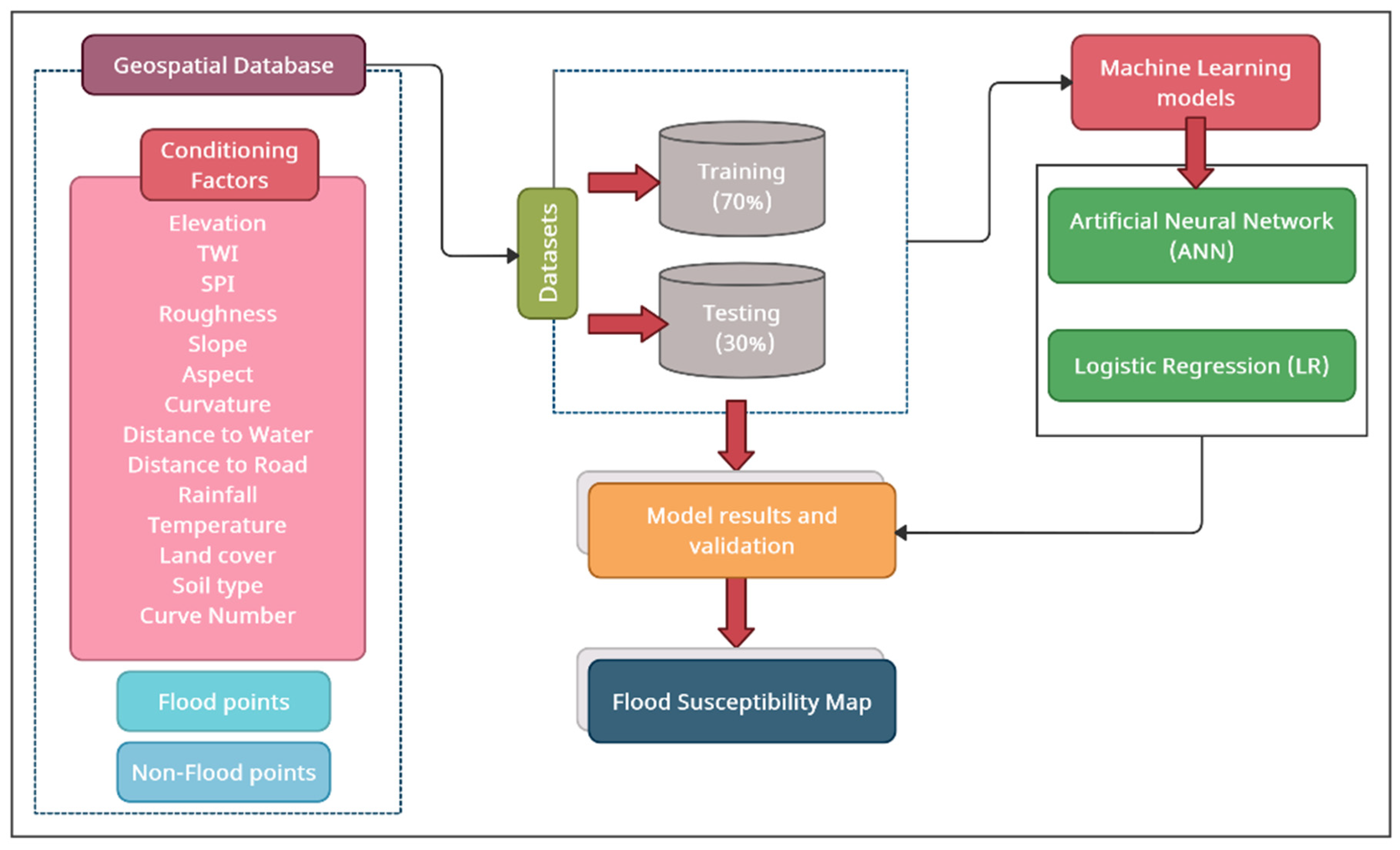
Nigeria is located between the Benin Republic and Cameroun in Western Africa (Figure 1). It has a total size of around 923,770 km² with a total landmass of about 910,770 km² and water bodies of about 13,000 km². Its coastline spans roughly 853 km along the Gulf of Guinea. Nigeria’s topography is divided into five regions: the coast along the Gulf of Guinea; the north-central plateaus; the rivers Niger-Benue, plateaus around the north borders; and mountainous zones to the east, with Chappal Waddi at 2419 m its highest point.

Nigeria has four distinct climate zones: savannahs, Sahel, equatorial monsoon, and alpine, distributed from north to south. In the south, maximum temperatures range from 30 to 32 degrees Celsius, while temperatures range from 33 to 35 degrees Celsius in the north. There are two main seasons: the dry (November to February) and wet seasons (March to September). The average annual rainfall declines as one travels north, ranging from roughly 2000 mm at the coasts (averaging 3550 mm in the Niger Delta regions) to between 500 and 750 mm in the northern regions [33].

Nigeria’s two main water systems are the Niger-Benue and the Chad basins. The rivers Niger-Benue is the primary water source for practically most of Nigeria. The upstream river Niger (north-west), the lower Niger (south-south), and the Benue River (north-east) are the three main river portions. The Benue basin is a tributary of the Niger River that began in the Mandara highlands (forms a confluence at Lokoja with the River Niger). Katsina-Ala, Taraba, and Gongola are the principal tributaries of the Benue River in Nigeria. During the rainy months, the upper Niger River rises to around 800 m in Guinea’s Fouta Djallon Massif and runs northeast through Mali’s interior Delta to the Niger Delta region bordering the Gulf of Guinea into the Atlantic Ocean. Other notable rivers, including the Zamfara and Kaduna, flow into the Niger River and travels south towards the lower banks through Nigeria.

Nigeria has a prevalent history of natural disasters. Flooding is the most frequent and destructive natural hazard in Nigeria (80%), according to the National Emergency Management Agency (NEMA). In July 2012, continuous extensive rainfall in the rivers Niger-Benue axis of Nigeria caused destructive flooding. As a result, 30 of Nigeria’s 36 states were affected by significant flooding from early July 2012 until late October 2012, following a long rainy season from April to September 2012. “Highlighted as one of the worst flooding incidents to occur in the modern history of Nigeria, with a total economic loss of US$16 billion, an estimated 2.1 million people were displaced from their homes, and 363 deaths were recorded as of September 2012. By the end of October, about 7.7 million persons had been affected, and over 2 million Nigerians were registered as internally displaced persons (IDPs)” [34]. The Niger-Benue River flood was caused by several factors, including (a) torrential continuous rainfall across multiple states resulting from over 14 days of continuous rain, (b) excess runoffs and overflows of water reservoirs and (c) dam failure due to excessive water inflow leading to the destruction of farmlands, infrastructural property, and flash floods. For example, the water levels from the riverbanks in the Niger-Benue axis rose to about 12.84 metres (42 ft). According to the data provided by the Dartmouth Flood Observatory, the climax of flooding occurred between late August and early September.

However, poor data collection and reporting issues make it difficult to effectively estimate the extent of the loss, especially to the human and natural environment. Man-made actions aggravate Nigeria’s frequent flooding, evident in the lack of preventive planning, high rate of deforestation, rapid and unregulated urban expansions and the limitations in the available infrastructural amenities to provide comprehensive defence against flooding.

2.2. Methodology

There were four main steps in the flood susceptibility mapping process (Figure 2). These include: (i) the creation of the geospatial database containing all essential elements (conditioning variables) and historical flood occurrences; (ii) building the machine learning models; (iii) models’ validation; and (iv) production of the flood susceptibility map. A detailed description of each stage is included in the subsections that follow.

2.2.1. Inventory Map of Historical Flood Events

It is critical to identify and map historical flood locations to investigate the geographical link between flood likelihood and the factors that impact it [35]. Numerous methods for creating flood inventory maps have been explored, including utilising existing historical archives, field surveys and remote sensing. Since the coverage area is relatively large in this study, we chose to utilise historical extensive flood archives obtained from the Dartmouth Flood Observatory (DFO) [36]. The information made available in the archives was derived from new sources, governmental organisations, and remote sensing. In addition, supplementary flood information was obtained from the EM-DAT public database (

Table 1. Sources of data for the flood inventory.

Period	Contents of the Data	Data Type	Source
1985–2020	Location, date, validation, displaced, deaths, severity	Polygon (points)	EM-DAT, CRED
1985–2020	Location, date, affected	Polygon (points)	Dartmouth Flood Observatory (DFO)

). To further verify the authenticity of the obtained information, we verified the data from historical news archives from the governmental organisation in Nigeria, NEMA. Sources of data for the flood inventory map are shown in Table 1.

Seven hundred and sixty-five (765) flood events between 1985 and 2020 were identified (Figure 3). In addition, we sampled 765 non-flood incident points from areas with a known history of non-flooding. The datasets from the two samples (flooded and non-flooded) were allocated values of 0 and 1, required for the model development—1 indicating the flooded area and 0 denoting non-flooded area. The total number of generated location datasets was pooled and divided into two groups, 70:30 training and testing datasets [37]. Consequently, 1071 data points were used as training sets and the remaining 459 as validation sets.

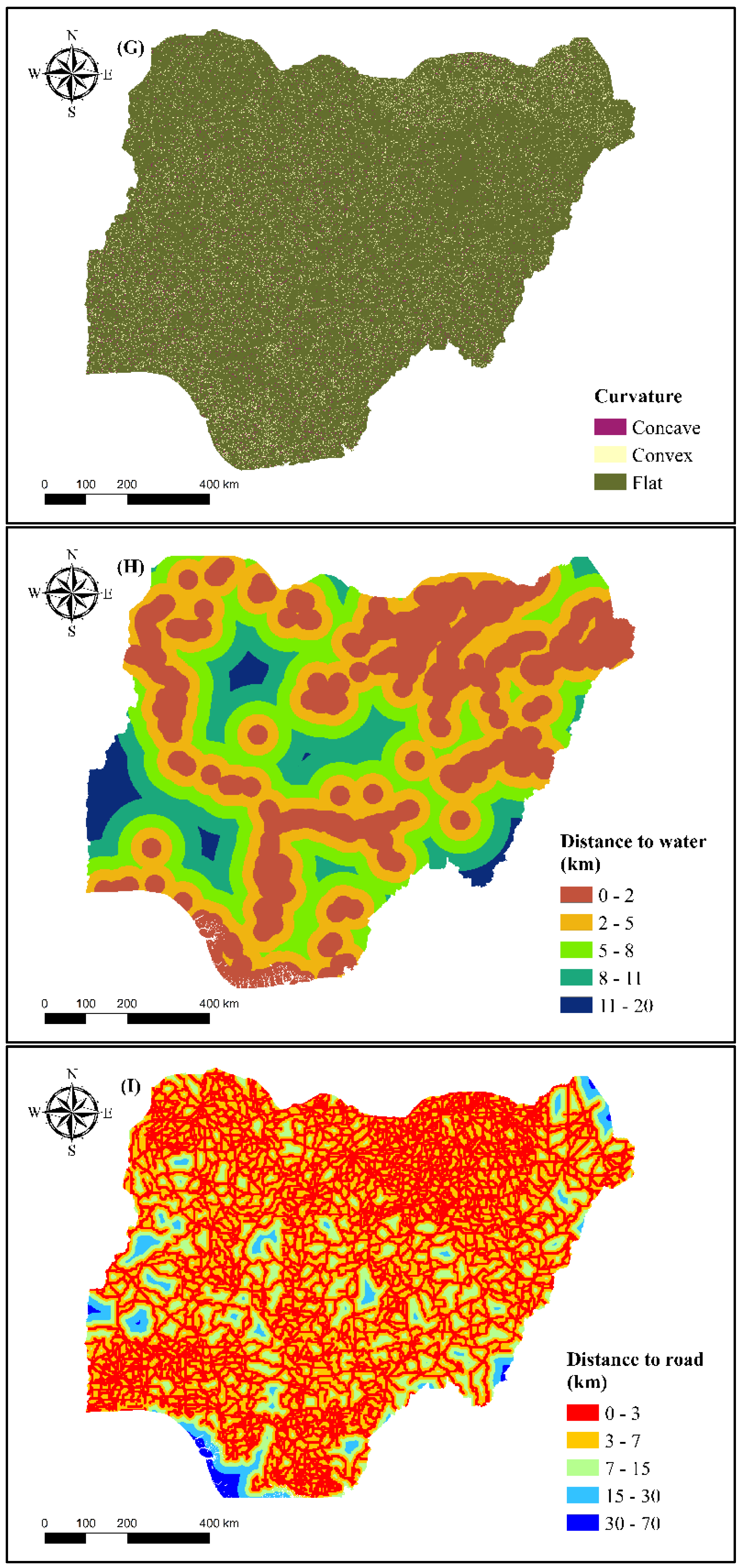
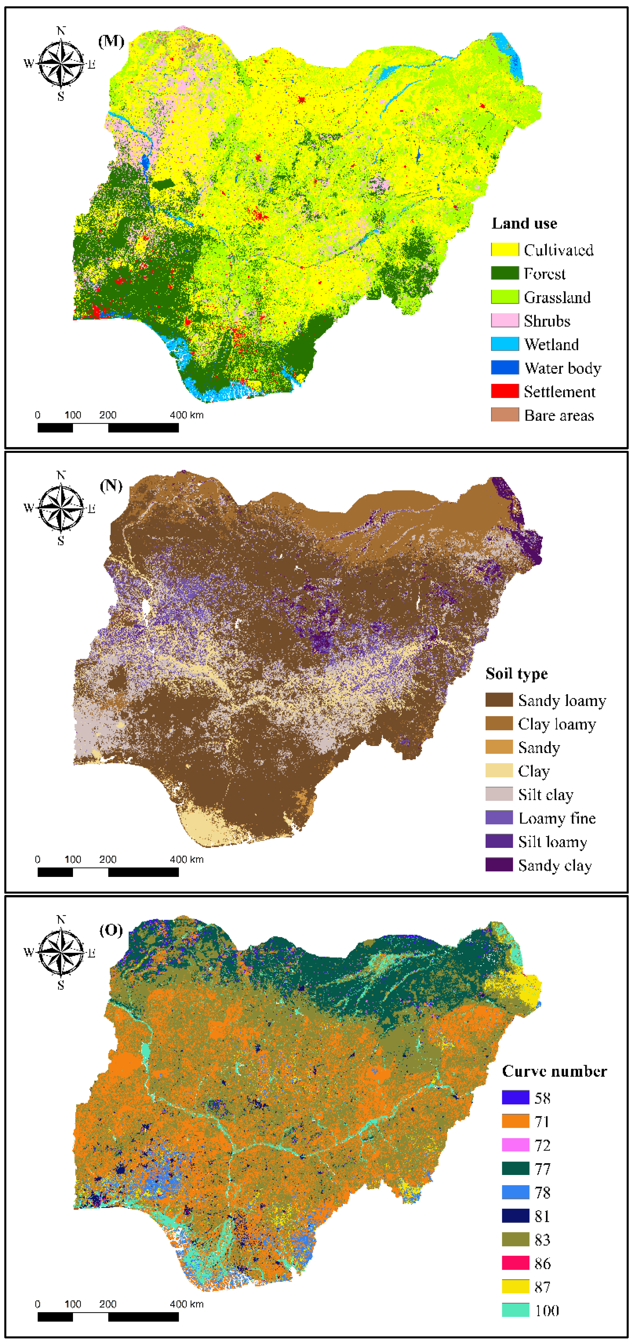
2.2.2. Flood Conditioning Factors

Flood conditioning factors are the topographical, hydrological, or socio-economic variables that influence the occurrence or magnitude of flooding incidents. Each factor acts independently and in unison to form a flood incident. Existing literature on flood modelling was considered [38,39,40,41,42]. In addition to consulting previous literature, the selection of the final set of conditioning factors was based on conducting surveys on the factors that had a significant impact on the local territory of Nigeria.

The selection of flood conditioning factors is commonly chosen based on past research and expert opinions. However, because each region comprises diverse natural and anthropogenic components [43], it is vital to acquire geographical knowledge about the study area and its surroundings in flood modelling. As a result, the criteria for selecting the conditioning factors for this study are discussed in the following sections. The flood conditioning factors in this study are categorised into two groups, namely, natural and anthropogenic factors. The natural factors include the topographic, hydrographic, and climatic components of the study area, while the anthropogenic factors are the components influenced by human activities, including road network and land use. A digital elevation model (DEM) with a 30-m spatial resolution produced by the USGS Earthexplorer was used to derive other related parameters. Afterwards, aspect ratio (Figure 4F), slope (Figure 4E), curvature (Figure 4G), SPI (Figure 4C), and TWI (Figure 4B) were derived from the elevation data. Finally, the QGIS and SAGA GIS software was used to produce the final maps of the slope, aspect, TWI, SPI, and curvature.

New research [44,45] found that the topography of a place has a vital role in determining the severity of floods and identifying flood-prone locations. The elevation is selected as a conditioning factor due to its importance in the occurrence of floods because previous literature shows that locations with a high elevation increase runoff, whereas flat areas are more prone to flooding owing to high water discharge [46]. In the case of Nigeria, the southern regions close to the major rivers and the Atlantic Ocean have very low elevations, which makes an excellent factor for flood susceptibility mapping. Similarly, as water travels from higher to lower elevations, the degree of slope affects surface runoff and water infiltration rate [47]. Therefore, low degree slope areas are prone to flooding, which makes slope as a conditioning factor becoming vital in flood conditioning factors selection [48].

Curvature is a morphometric feature that impacts the occurrence of floods by identifying the divergent and convergent runoff zones. Curvature can either be flat (zero curvature), convex (positive curvature), or concave (negative curvature). Flooding is more likely to occur in flat and concave areas [49], as these areas tend to hold water longer than those with convex shapes [50]. The aspect of the topographic surface is the horizontal direction in which a slope face. It considers weathering consequences because of the quantity of rainfall, making it an essential factor in flood analysis [51].

Furthermore, the hydrological factors stream power index (SPI) and topographic wetness index (TWI) were also considered conditioning factors in the study. The SPI is one of the most essential and extensively utilised parameters in most flood modelling studies, as it measures the erosive strength of runoff [52]. It also indicates the erosive power and concentration of surface runoffs, which plays a vital role in terrain stability. As a result, it helps determine where soil conservation measures might help prevent erosion from surface runoff. The TWI defines the flow and accumulation of water at a given place within a watershed due to gravitational force. The TWI detects flood-prone locations within a watershed because steeper slopes have a lower filtration rate than level terrains [53]. As a result, TWI reveals the infiltration capacity in a region and flood-prone zones. Roughness deals with variations in surface changes and irregularities. These elements, such as trees, shrubs, and logs, can be found on the topographical surface. Modelling the floodplain’s hydrology requires mapping the geographical distribution of these roughness characteristics at various scales [54] and how they contribute to flooding incidents. As such, the roughness was considered a conditioning factor in this study.

Soil properties vary by area due to differences in particle composition, which impacts the amount of water filtration. The amount and pace of water infiltration and runoff determine the soil’s texture, type, and structure. Soil types were selected as a conditioning factor because Nigeria possesses multiple soil characteristics which can shed light on the nature and cause of flooding across its region. The curve number (CN) was chosen as the key index for runoff circumstances. The curve number (CN) is an empirical metric for calculating direct runoff or infiltration from excess rainfall in hydrology.

In addition, land use plays an essential part in flood occurrence; urban areas are more prone to flooding owing to the presence of imperviousness surfaces such as roads and building structures, whereas vegetated regions are less likely to trigger flooding incidents, especially in areas with higher vegetative cover such as forests. As a result, land use is selected as a flood conditioning factor, as it can highlight the link between land utilisation and the probability of flooding.

In most flood studies, rainfall has been identified as an essential factor in flood occurrence [55]. Rainfall has a substantial impact on flood occurrence due to its geographical and temporal patterns; as a result, an increase in rainfall leads to a considerable rise in the likelihood of flooding [56,57,58]. Climate change has the potential to affect flood risk and water resource management. Mitigation planning should be able to forecast changes in floods and their occurrence. Recorded temperature correlations inform changes in hydrologic extremes, ranging from basic proportional change techniques to conditioning stochastic rainfall production based on observed temperatures. As temperature changes can potentially alter the amount of precipitation/rainfall at a given location, affecting the probability of flooding incidents. The temperature was considered a conditioning factor, as Wasko [59] highlighted the sensitivities between temperature changes, precipitation, and increase in flow volume at the peak of flooding incidents [59]. In Nigeria’s case, the considerable variation in temperature distribution across the geographical region is a cause for integration and further investigation into the factors that affect flood occurrence.

Studies show that flooding is influenced by the distance from the river, which can determine the extent and size of the flood [60]. A river floods when the volume of water surpasses the capacity of the river network [61]. In Nigeria, most flooding incidents occur when the riverbanks overflow into settlement and agricultural land areas within proximity to existing rivers. As a result, the river’s distance must be considered an influencing element.

Distances from road and rail networks can influence flooding. Road and other artificial surfaces increase water inundation due to their imperviousness and create a conduit for water flow. Hence, lowering the infiltration rate, resulting in a higher runoff rate [62]. Similarly, human settlements are likely to be situated close to roads, which exposes them to a higher probability of flooding. As a result, the distance to the road was selected as a flood conditioning factor.

Overall, the study used a total of fifteen (15) variables: elevation, roughness, slope, curvature, curve number, stream power index (SPI), rainfall, topographic wetness index (TWI), aspect ratio, soil type, land cover, distances to the road, water, and rail, and temperature to predict flood susceptible areas in Nigeria. (

Table 2. Data sources and their specific use.

Data	Sources	Format	Period
Rainfall	Nimet, Nigeria	vector	1975–2015
Temperature	Global Climate data: Worldclim	1 km	1975–2017
Land cover	Globeland30	30 m	2020
Soil *a	The Harmonised World Soil Database v1.2	vector	-
Soil *b	Global Hydrological Soil Group- ORNL DAAC	250 m	2020
Elevation	USGS, Earthexplorer	30 m	2015
Road network	NASA, Socioeconomic Data and Applications Center; Global Roads Open Access Dataset v1	vector	2010
Rail network	OCHA, Nigeria	vector	2009
Water areas	OCHA, Nigeria	vector	2010

Soil data: *a: provides regional soil information and soil parameters provided by FAO-UNESCO; *b: Hydrological soil groups (HSGs) data applied to estimating the curve-number for rainfall runoff estimates, provided by the ORNL DAAC.

, Figure 4A–O). Further details on each conditioning factor are found in the subsections that follow.

To ensure uniformity of the raster datasets with different resolutions in the modelling process, we utilised the resample function in ArcGIS to derive a standard resolution and projection at 30-m. Here, we selected the bilinear interpolation method to calculate the pixel value, which uses the distance-weighted values of the nearest pixel, a relatively efficient approach for reducing errors.

Topographic elements (slope, aspect, altitude, curvature, roughness, SPI, and TWI) are frequently utilised as conditioning variables in flood modelling because floods have a high correlation with a location’s current topography (Figure 4A–G) [63]. Previous flood modelling literature indicates that floods often occur in flat and low-lying locations, influencing the study’s selection as a conditioning element [64,65]. Aspect and curvature are related to the union, direction of flow, and contour of the ground surface contour, which influences the likelihood of flooding. TWI, SPI, and roughness are secondary parameters generated from the elevation, which provide information about the hydrological environment.

The elevation is a critical component in flood vulnerability studies. Areas with lower elevation values, particularly coastal areas, are more prone to floods than areas with higher elevations, usually prone to landslides [66,67]. We developed the topographic conditioning factors using a 30-m resolution digital elevation model (DEM) retrieved from NASA Earth explorer.

The topographic wetness index (TWI) measures the amount of water accumulated at a specific site and the likelihood of water flowing downward due to gravity. The higher the TWI number, the greater the risk of floods. The TWI is expressed as

$$\mathrm{TWI}=\mathrm{Ln}\frac{A_s}{\tan \beta }$$

(1)

where: $A_s$ is the local upslope area draining through a certain point per unit contour length, and $\tan \beta$ denotes the local slope in radians.

The stream power index (SPI) measures the erosive power of flowing water at a given point on a topographic surface. The SPI is expressed as

$$\mathrm{SPI}=A_s\times \tan \beta$$

(2)

where: $A_S$ is the local upslope area draining through a certain point per unit contour length and $\tan \beta$ denotes the local slope in radians.

Roughness measures the degree of change on a topographic surface. It also represents the resistance to flooding flows within a channel and floodplain.

In flood susceptibility mapping and hydrological investigations, the slope is one of the most often utilised conditioning variables. Since this study involves estimating flood susceptible areas, the slope was selected as there is a close relationship between the direction of the slope and the infiltration of rainfall on the topographical surface. The slope values ranged between 0 and 90 degrees.

Aspect represents the direction of the maximum slope. It is also a measure of the steepness of the topographical surface. The aspect has nine (9) categories at 45-degree intervals.

Curvature is another component that influences flood studies. It denotes the topography’s morphology. It is either flat, convex or concave.

Proximity factors: distances to water, road and railway, were also considered. The distance to water is necessary when estimating the factors that influence flood probability due to flooding typically resulting from an overflow of neighbouring water surfaces [68,69]. Similarly, the distance to infrastructural services such as road and railway were also estimated. The distance to the road and railway is an influencing element because artificial surfaces adjacent to bodies of water have a substantial effect on the soils’ hydraulic conductivity. As urbanisation continues, areas with a lower hydraulic conductivity due to infrastructure development are likely to be flooded [70]. The generation of the distances to water, road and railway map is in the SAGA GIS and QGIS 3.14 software (Figure 4I,J).

Rainfall and temperature (Figure 4K,L) are essential variables, especially for Nigeria, as the massive climate variations between regions play a vital role in determining flood probability. At this point, we took historical precipitation data (1975–2017) from 28 rainfall stations across Nigeria and interpolated the annual rainfall map using the inverse distance weighted (IDW) method. The IDW interpolation method was selected as it allows for the estimation of unknown values within a specified distance, based on the mathematical assumption that the closer values are more related than other values (Figure 4K). In addition, the mean annual temperature data were collected and analysed from the Worldclim for this study.

Land use and soil cover information were used as conditioning factors to help understand how human activities and the existing landscape modifications impact flood probability. The land use maps comprise eight (8) categories: forest, shrubs, cultivated, water, wetland, grassland, settlement, and bare areas. Land use maps were from Globeland 30 and soil information from the Harmonised world soil database v1.

The curve number (CN), used in many hydrological studies that assess runoff or infiltration from excess rainfall, was selected as one of the conditioning factors. The Curve Number estimates were derived using global hydrological soil groups (HYSOGs) data at 250 m spatial resolution [71] and land cover data for 2020 for Nigeria.

The conditioning factors (Figure 4A–O) mentioned above help assess the possibility of flood occurrence using the machine learning ANN and LR algorithms. Using machine learning methods allows assessing each conditioning factor and evaluating their correlations without classifying the independent datasets (conditioning factors). Furthermore, the methodology used in this study can be reproduced and implemented in other predictive modelling tasks such as landslides because it does not require extensive data on the hydrology and topology of the study area.

2.3. Machine Learning Models

2.3.1. Artificial Neural Network (ANN)

The artificial neural network (ANN) is a subset of techniques used in machine learning. These non-linear statistical models exhibit a complicated interaction between inputs and outputs to identify new patterns. ANNs can perform a wide range of tasks, including image identification, speech recognition, predictive mapping and medical diagnosis. They consist of multi-layered interconnected neural nets, comprising an input layer, one or more hidden layers, and an output layer [72].

The input represents the basic information required in the network represented by the activity of the inputs. The hidden identifies and houses the activities between the initial model datasets and their derived weights within each connection. Finally, the output measures the interaction and behaviours between the parameters in the model.

After collecting the conditioning factors, the artificial neural network simulated the link between the presence or absence of a flood episode (response variable) and the fifteen covariates chosen (conditioning factors- TWI, SPI, Curvature, Slope, Elevation, Land use, Curve Number, soil type, Rainfall, Distances to water, road and rail and temperature based on the cross-entropy (“ce”) method for the flood susceptibility mapping.

A typical artificial neural network model usually consists of three main layers: an input, a hidden, and an output [73]. The input layer contains all covariates (contingent variables), whereas the output layer comprises the response variables. The hidden layer(s) is between the input and output layers and is not visible. As the neural network models the relationship between covariates (x) and the response variable (y) [74], a weight is added to the modelling process to represent the effect of the variables given as signals within the neural network. A simple depiction of neural net training is

$$O\left(\nu \right)=f\left({\omega }_0+{\displaystyle \sum }_{r=1}^k{\omega }_r{x}_r\right)=f\left({\omega }_0+W^{T}v\right)$$

(3)

where: $O\left(v\right)$ is the output of the neural network, ${\omega }_0$ denotes the intercept, $k$ is the total number of flood conditioning factors, ${\omega }_r$ the flood conditioning factors’ weight coefficient and $f$ specifies the activation function in the hidden and output layers, ranging from 0 to 1. The function is calculated by

$$W^{T}v=\left({\omega }_1{v}_1+{\omega }_2{v}_2+\dots \dots ..+{\omega }_k{v}_k\right)$$

(4)

where: $\omega$ is the vector containing all the weights without the intercept, $\nu$ is the vector of all covariates, and $W^{T}v$ is a scaled product of the weights and input vectors.

As the ANN calculates the output $O\left(x\right)$ based on the given inputs and current weights, there is a need to define the error function, which describes the deviations between the predicted and observed outcomes. A model with a significant deviation indicates a poor fit and would require adjustments. Therefore, our study chose the cross-entropy function over the conventional back-propagation approach.

The cross-entropy was selected as the modelling approach for the ANN because it is relatively faster than the conventional back-propagation technique in terms of system processing duration [75,76]. The cross-entropy classification method is a measure from the field of information theory built on the entropy backbone to calculate the difference between two probability distributions. The cross-entropy method measures the differences between two probability distributions for a given random variable or set of events. It extends the concept of entropy from information technology by calculating the number of bits required to describe or transmit an average event from one distribution to another. The cross-entropy error function is expressed as

$$E_{ce}=\frac{1}{2}{\displaystyle \sum }_{l=1}^L{\displaystyle \sum }_{h=1}^H(y_{lh}\log \left(O_{lh}\right)+\left(1+y_{lh}\right)\log 1-O_{lh}))$$

(5)

where: $l$ = 1 is the index of the observation (inputs and outputs), and $h=1$ is the output nodes.

After successfully training the model, we visualised the results to understand the contributions of each conditioning factor to flood occurrence. Although the ANN can make sound predictions compared to other models, it is often challenging to interpret the results [77]. The generalised weights help define the effect and contribution of each covariate on the response variable (flood). The generalised weights expressions are as follows

$${\tilde{\omega }}_i=\frac{\partial \log \left[\frac{o\left(x\right)}{1-o\left(x\right)}\right]}{\partial {\mathrm{x}}_i}$$

(6)

where: $i$ is the index for the covariate (conditioning factors), and $o\left(x\right)$ denotes the result (predictions) as a function of each covariate [78].

The effect and connection between the input and output variables reflect in the output weight distribution. If the distribution of the weights accumulates around zero, it shows that the selected variable does not affect the outcome status. If the distribution is large, the input variables have a non-linear effect. Another advantage of this method is that it represents the statistical significance of each variable in the datasets concerning its effect on the model. It is easier to visualise each predictor based on their contributions to the model outcome, allowing for easy understanding, comparison and elimination of predictors that contribute nothing to the model.

To compare the ANN’s performance and predictive power with other machine learning models, we employed the logistic regression (LR) model, another widely used approach for assessing flood risk, using the same data parameters as the ANN.

2.3.2. Logistic Regression (LR)

The logistic regression model enables the creation of a multivariate link between the independent and the dependent variable. While the dependent variable is binary, the independent variables can be binary or categorical [79,80]. Like the multiple linear regression, the logistic regression model enables an understanding of the relationship between flood and the specified independent variables. The dependent variable in this study is binary [0,1], denoted by the existence or absence of a flood occurrence. The logistic regression model is denoted by

$$P=\frac{exp\left(z\right)}{1+exp\left(z\right)}$$

(7)

where: $P$ is the chance of an event (flood) occurring, which ranges from 0 to 1, and z denotes the linear combination of the selected flood conditioning elements, further expressed as

$$\mathrm{z}={\beta }_0+{\beta }_1{\chi }_1+{\beta }_2{\chi }_2+\dots \dots \dots ..+{\beta }_n{\chi }_n$$

(8)

where: $\mathrm{z}$ represents a combination of all the independent variables (conditioning factors); $X_1,\dots .X_n$, ${\beta }_0$ representing the intercept and ${\beta }_{1 }, \dots ..{\beta }_n$ are the logistic parameters.

2.4. Correlation Analysis

It is crucial to investigate the relationships between and within the selected independent variables in predictive modelling to ensure the model produces accurate results. Correlation analysis is the process of investigating the relationship between the selected independent variables. When two or more selected independent variables have a high correlation, multicollinearity occurs [81]. Furthermore, when a group of independent variables have a very strong correlation between them, they are considered multicollinear, which, if left in the dataset samples, increases the probability of analytical mistakes in natural hazards modelling [82]. Multicollinearity may be measured using various approaches, including the variance inflation factor (VIF), the conditional index, Pearson’s correlation coefficients and variance decomposition proportions [83,84,85]. We chose the VIF and Pearson’s correlation coefficients in this study, popular in flood and other statistical analytical studies [86,87].

The VIF determines the degree of interdependence between the variable and other predictor variables. A higher variance means an increase in the standard error of the variable within the model. The square root of VIF represents the degree to which collinearity raises the standard error for that variable. A VIF of 5, 10, or greater means multicollinearity has emerged [88].

2.5. Pearson’s Correlation Coefficients Estimation

The Pearson correlation coefficient indicates how strong a linear link is between two variables. It ranges from −1 to 1, with −1 indicating a complete negative linear correlation, 0 indicating no correlation, and +1 indicating a real positive linear correlation. The pearson correlation coefficient is estimated by

$$r=\frac{{\displaystyle \sum }\left(x_i-\overline{x}\right)\left(y_i-\overline{y}\right)}{\sqrt{{\left(x_i-\overline{x}\right)}^2{\displaystyle \sum }{\left(y_i-\overline{y}\right)}^2}}$$

(9)

where: $r$ is the correlation coefficient, $x_i$ and $y_i$ are the values of variables $x\mathrm{and}y$ and $x$, and $y_i$-denotes the mean values of each variable.

The Pearson correlation coefficient analysis is presented in a table known as the correlation matrix. Each value indicates the linear relationship between each of the independent variables.

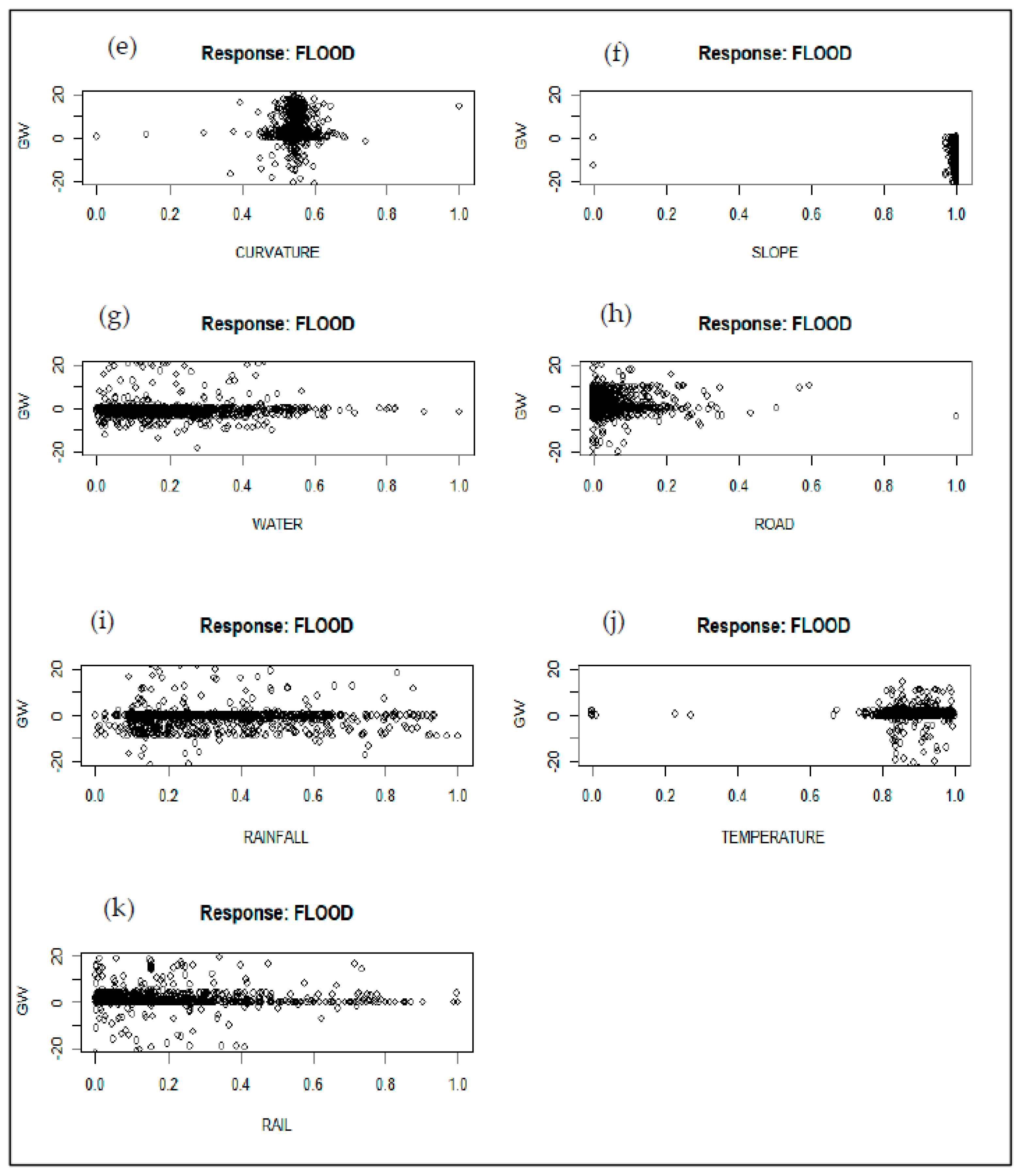
2.6. Variable Importance Estimation

The relative importance is a measure for estimating the contribution of the input variables used for predicting the dependent variable. There are numerous ways to estimate input variables’ relative importance in machine learning models.

The sensitivity analysis, Garson’s algorithm, Lek’s profile approach, connection weights algorithm and usage of partial derivatives are some of the most used variable importance estimation methods. In this study, we chose the connection weights algorithm. Olden et al. [89,90] highlight that the connection weight method has the best performance compared to the other approaches in terms of estimating and ranking the importance of all the variables in the model based on the accuracy (the degree of similarity) between the actual and estimated variables and precision (the degree of variations in accuracy). Similarly, the connection weight strategy performed the best when properly assessing each variable’s actual significance in the neural network. It is the product of the input to hidden and hidden to output connection weights established between input and output neurons and sums the products across all hidden neurons. As a result, the relative importance is determined by

$${\mathrm{RI}}_{\mathrm{x}}={\displaystyle \sum }_{y=1}^m{w}_{xy}{w}_{yz}$$

(10)

where: ${\mathrm{RI}}_{\mathrm{x}}$ is the relative importance of the input variable $x$. ${\displaystyle \sum }_{y=1}^m{w}_{xy}{w}_{yz}$ is the sum of the final weights of the connection from the input to hidden neurons, y is the total number of hidden neurons, and z is the total number of output neurons. This method correctly identifies the fundamentally important variables in the model.

2.7. Assessment of Modeling Accuracy

We evaluated the models’ accuracy with the area under the curve (AUC) and the receiver operator curve (ROC). The AUC is one of the most popular methods of quantitatively assessing the accuracy of success and predictive capacity of a diagnostic model. Multiple studies on flood susceptibility mapping have utilised the AUC approach and verified its efficiency in validating diagnostic models. The AUC was estimated in both models applied in the study (ANN and LR) by comparing the model performance results using the training and testing datasets.

As noted previously in the methodology section, flood inventory data (consisting of 1486 flood and non-flood locations) were divided randomly into 70:30 ratios to train and test the model. The success rate was determined using the training dataset of 1071 points, while the prediction rate of the model was determined using the testing dataset of 459 points.

2.8. Model Performance Evaluation

A high performing machine learning (ML) model is accessed based on the accuracy in predicting possible outcomes based on training and validation datasets. One key factor responsible for high-performance ML models is the selection of multiple parameters that influence the model outcome [91]. In ML, this process is called hyperparameter tuning. Hyperparameter tuning involves deriving a first-rate set of parameters to achieve the best result for the model. These may include decisions on choosing the number of layers and neurons, optimisation and loss functions, learning rate, metrics and layer weights, all of which influence the model’s outcome. Hence, to derive the best parameter values for the model in this study, a trial-and-error method is adopted by testing multiple parameters before achieving an acceptable result.

We employed multiple statistical indicators to assess the performance of the ANN and LR models, including the area under the curve (AUC), receiver operating characteristic curve (ROC), accuracy, mean square error (MSE), and the root mean square error (RMSE). In this study, all the evaluation metrics were derived based on a confusion matrix of the models’ outputs. In addition, the MSE and RMSE indexes helped evaluate the model performance. After repeated model runs, we developed an ANN model structure with eight hidden layers with 64 neurons (

Table 3. Parameter settings for machine learning models (ANN).

Parameters	Model Values
	ANN	Logistic
Training	70	70
Testing	30	30
Number of hidden layers	8	0
Number of neurons	64	0
Activation function	logistic	logistic
Learning rate	0.001	0.001
Architecture selection	Trial-and-error	Trial-and-error

).

3. Results

3.1. Artificial Neural Network Model (ANN)

The artificial neural network model identifies flood conditioning elements and their effect on flood susceptibility. The analysis result shows the graphical visualisation of the ANN model training results, which explains the relative contribution of each covariate (condition factors) on flood susceptibility. In addition, the first result group (continuous data) (Figure 5) shows the generalised weights of the ANN, which is an effective method for determining the relationship between each covariate and flood.

The generalised weights distribution describes that curvature, slope, TWI, distance to water, distance to road, roughness, elevation, rainfall, distance to railway and temperature have significant positive non-linear effects on flood occurrence. Figure 5a–k shows that most covariates have negative and positive effects on flood occurrence. In interpreting the ANN generalised weights results, if all the weights are around zero (0), the covariate does not affect the outcome (flood) status. However, having most of the weights above zero (0) denotes having a positive effect on the response variable and vice versa if the majority are below 0 [92].

In this study, curvature, distance to water, roughness, road distance, SPI, TWI, rainfall, distance to rail, and temperature all exert positive and negative non-linear effects. Similarly, the lower TWI values have adverse effects on a flood. Moreover, higher temperature values positively affect flood outcomes, while slope and elevation negatively have a non-linear effect on a flood.

3.2. Logistic Regression Model (LR)

The logistic regression model results show each variable’s overall contribution to flood susceptibility levels in Nigeria.

Table 4. Coefficients of each independent variable used in the logistic regression model.

Factor	β Coefficient	Significance (p-Value)
Aspect	−0.0012	0.0022 **
Curve Number	0.0190	0.0219 *
Curvature	0.0009	0.0005 ***
Elevation	−0.0004	0.3717
Land use	−0.0076	0.0022 **
Rainfall	0.0001	0.0075 **
Roughness	0.0015	0.0028 **
Soil type	−0.0043	0.035 *
Slope	0.0007	0.0945 *
SPI	−0.2856	0.0271 *
Temperature	−0.0163	0.3035
TWI	0.0027	0.0934 *
Distance to Water	0.0728	0.008 **
Distance to Road	−0.2047	0.0002 ***
Distance to Railway	0.0397	0.7256

Significance codes: ‘***’ p < 0.001, ‘**’ p < 0.01, ‘*’, p < 0.05.

contains the findings for each independent variable included in the logistic model. To understand the significance of the variables in flood susceptibility mapping, we set the significance to 5% significance (p = 0.05). Curvature and road distance had the highest significance in the LR model. Similarly, aspect, land use, rainfall, roughness, and distance to water were also significant to flood occurrence. The insignificant variables in the model were the elevation, temperature and distance to the railway, respectively. The results from the logistic model highlight what variables impact flooding. The results from the logistic regression analysis show that the distance to road, curvature, land use, distance to water, rainfall, roughness, and soil type have a significant impact on Nigeria’s flood susceptibility, as they have p−values < 0.05 (5%) significance levels. In addition, we observe that the curve number, slope, TWI, SPI, and aspect were equally significant in the LR model.

3.3. Flood Susceptibility Map

The susceptibility map is the final output of the modelling process. The flood susceptibility map can help disaster planning and serve as an initial step in flood mitigation. The visualised map quickly identifies the most vulnerable locations and prompts appropriate responses. The susceptibility map produced in this study shows a flood probability index divided into five flood occurrence probabilities. We created the final maps after training and validating the machine learning models. The flood susceptible areas are derived based on the ANN & LR models. Each pixel allocates a value between zero (0) and one (1), which indicates the probability of flooding at a particular location. A score of 0 suggests a low flooding probability, whereas 1 indicates a higher probability [29].

To develop the probability map, we divided the flood susceptibility index map into five classes by adopting the quantile-based method [53], a commonly used approach in hazard research using ArcGIS 10.8, with categories ranging from very low to very high [40]. The maps of flood susceptibility generated by both the ANN and LR models are in Figure 6. In the map’s classification schemes, dark green indicates low flood susceptibility, and dark red indicates areas with very high susceptibility (Figure 6a,b).

Comparing the map produced by the ANN and the LR models, we can observe the differences in the susceptibility indexes produced due to the differences in the model classification despite applying the same data samples. For example, in the ANN-produced map (Figure 6a), regions around the northern region, coastal, and water bodies appear to have a higher flood susceptibility than the map produced by the LR model (Figure 6b). In contrast, the LR model map shows that aside from the coastal areas and Southern extremities, areas around water bodies were not classified as high susceptible zones but between low and moderate susceptible zones. Overall, despite the differences in the result produced by both models, we established a basic idea of the areas susceptible to floods in Nigeria.

3.4. Validation and Accuracy Assessment

We used flood training and testing datasets to validate the flood susceptibility models. 70% (train set) of the data were utilised for training, whereas 30% (test set) for validation. Similarly, the model’s accuracy in forecasting flood-prone locations was determined using the receiver operating characteristic (ROC) and the area under the curve analysis (AUC).

The ROC curve is a good way to describe the quality of the model performance, its success and predictive capacity. The ROC presents a chart that shows the proportion of true positives in a positive sample set against the false positives in a negative sample set while adjusting the discrimination threshold. The ROC can quantify the strength of a system to anticipate a predetermined event(s) correctly. The AUC is a metric that indicates a model’s performance and overall possible categorisation levels. A higher AUC indicates that a model can predict future events better. For example, if the AUC is between 0.9 and 1, the model is excellent, good between 0.7 and 0.8 and failed if less than 0.5 [93].

As shown in Figure 7a, the artificial neural network (ANN) model achieves a better AUC value (0.964) than the logistic regression (LR) model (0.677). Since we applied the training data to test the model performance success, it is not suitable to utilise the same data to test the predictive strength of the models. However, in the predictive rate results, the artificial neural network (ANN) model also possesses a higher predictive capacity than the logistic regression (LR) model, with individual AUCs of 0.764 and 0.625, respectively (Figure 7b). The model’s performance success and predictive rates prove that the artificial neural network (ANN) model has more robust capabilities than the logistic regression (LR) at predicting flood susceptibility areas in Nigeria.

4. Discussion

Identifying flood susceptible areas is one of the most common approaches to developing flood mitigation plans and ensuring adequate, timely and proper resources allocation to the most vulnerable locations. Multiple studies apply machine learning techniques to predict flood locations and generate reliable flood susceptibility maps. However, variations in data availability between locations have proven to be a challenge for regions where flood historical, environmental, and hydrological data are scarce.

In this study, we applied two machine learning models, the artificial neural network (ANN) and the logistic regression (LR), to estimate flood susceptible areas and compared their success and predictive performances for Nigeria. We chose 15 flood conditioning factors to develop our flood susceptibility maps. The results show that the ANN model had higher success and predictive capability than the LR model. Our findings from both models coincide with many flooding susceptibilities mapping studies, demonstrating that the ANN model can effectively estimate flood-prone locations. For example, Falah et al. [69] demonstrated in their study on data-scare urban regions; the effectiveness of the Artificial Neural Network (ANN) model and its capability in processing large amounts of data in a short amount of time utilising historical flood occurrences to predict future events. Other similar studies [17,26,52] have compared multiple machine learning models with the ANN to estimate the predictive success of flood susceptibility mapping, and on most occasions, the ANN model had good performance accuracies. Furthermore, our study confirms prior findings, which show that machine learning algorithms can predict flood-prone areas with good capability and reliability [18]. Similarly, several studies have successfully predicted and mapped flood susceptibilities in various places throughout the world, such as Iran [15], China [56] and Vietnam [57], using a combination of the ANN and other machine learning algorithms, including random forest (RF), convolutional neural network (CNN), recurrent neural network (RNN) [45], support vector machine (SVM) [21,38], multivariate discriminant analysis (MDA) [13], logistic regression [17] and the autoencoder neural networks [2] methodologies.

The ANN model approach offers numerous benefits that make it suitable for addressing various issues and situations. For example, because many of the relationships between inputs and outputs in real life are non-linear and complex, the ANN can represent non-linear and intricate interactions. Moreover, the ANN does not limit the number of input variables, making it have a good capability to predict multiple possible outcomes. Similarly, the other selected model in this study, the LR model, has also been proved to be very straightforward and equally efficient in flood susceptibility mapping.

According to our findings, the high susceptibility flood areas are mainly dominant in regions of extensive human activities, such as the cultivated and settlement land areas. Similarly, areas around the coasts and water bodies were most prone to flood occurrences, indicating an increased necessity to improve the design of flood mitigation measures and infrastructural defences, providing comprehensive flood protection for people and infrastructure. Similarly, due to the extensive human activities in Nigeria, the probability of floods in the current study may change over time, which highlights the need for periodic flood susceptibility assessments to enable the implementation of better-informed flood mitigation strategies.

Our findings as a tool for flood mitigation planning are highly significant because with the present unavailability of comprehensive hydrological data for several regions of Nigeria, relying mainly on hydrological techniques to address flooding issues effectively may be difficult. For this reason, the introduction of machine learning algorithms for flood-prone areas prediction is beneficial. Therefore, the flood susceptibility maps produced can identify areas where mitigation measures are needed and assist disaster management and evacuation strategies. In addition, promote the adoption of machine learning approaches for other flood-related research where data is limited and utmost speed is critical.

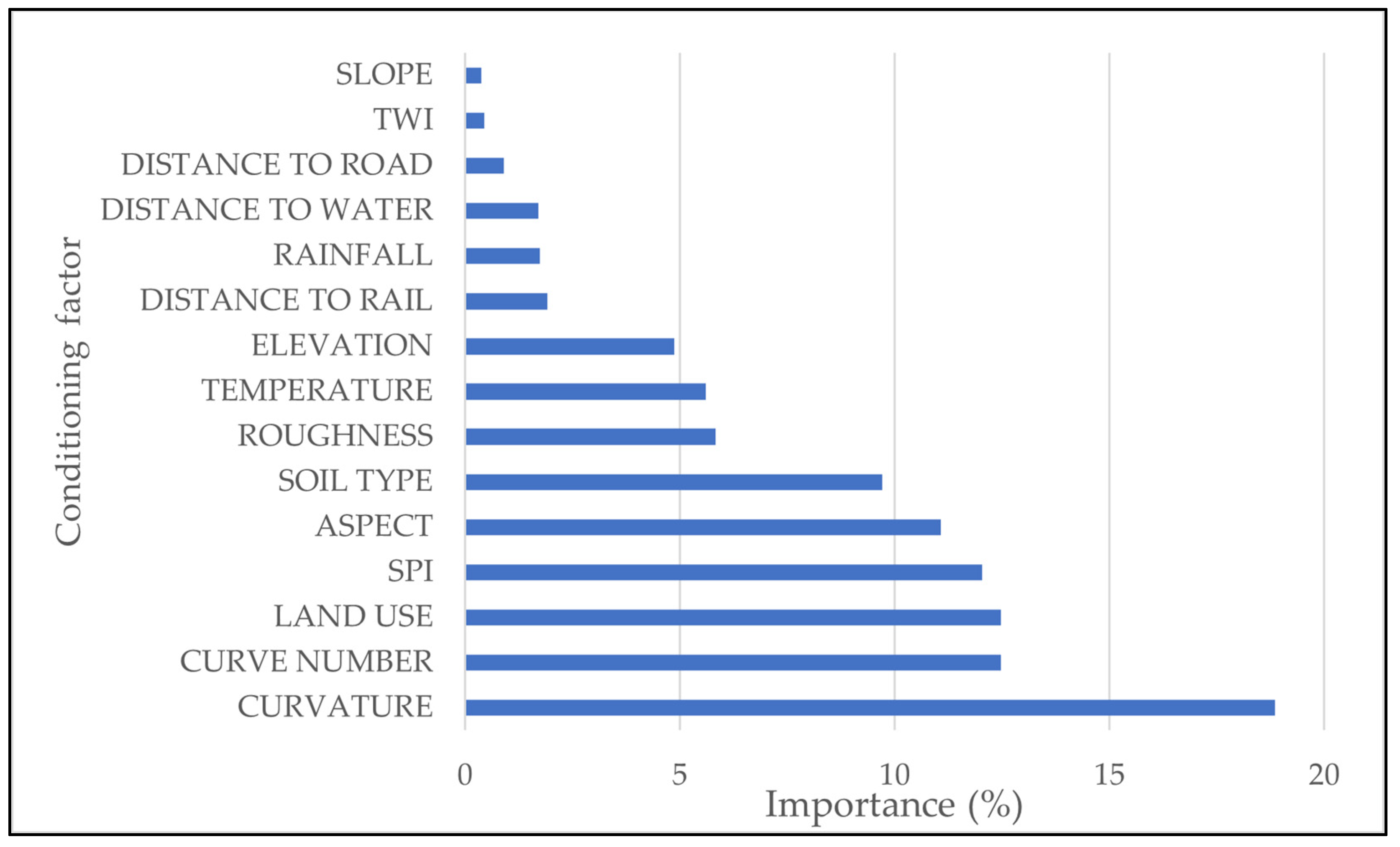
4.1. Variable Importance in Flood Susceptibility

Variable importance refers to methods for calculating a score for each model’s input features. The scores simply express the “importance” of each feature in the modelling results. A higher score indicates that a specific characteristic will significantly impact the model used to forecast a particular variable. The link between the features and the target variable may be understood using the variable importance. It also aids in determining which features are unnecessary for the model. The relative contributions of the input variables to flood susceptibility are in Figure 8.

The findings of relative importance estimation showed that soil and topographical components were the most critical factors that influenced flood susceptibility. Figure 8 indicates that curvature is the most important explanatory variable. Curve number, SPI, aspect, land cover and roughness are among the top essential factors in our analysis (Figure 8). On the other hand, variables TWI, distance to rail, slope and elevation have lower importance values, which is consistent with the results of the ANN generalised weights plot and the logistic regression coefficient values. From the results, curvature (18.86%), curve number (12.48%), land cover (12.47%), SPI (12.03%), and aspect (11.08%) are the top five most essential conditioning factors.

4.2. Analysis of Flood Susceptibility Model Results

Figure 9 depicts the distribution of the two flood-prone models’ flood susceptibility classification. According to the data, the very high category has the least proportion (18.47 per cent), followed by high (18.78 per cent), low (20.60 per cent), very low (20.90 per cent), and medium (21.25 per cent) classes in the logistic model. The percentages for the very low, low, moderate, high, and very high classes in the ANN model (Figure 9) are 6.5 per cent, 23.45 per cent, 26.07 per cent, 4.1 per cent, and 39.88 per cent, respectively. It can be found on both models’ flood susceptibility maps that the areas near the two main rivers (Niger and Benue) and the Atlantic Ocean (southern region) have incredibly high and very high flood-prone zones. Also, the areas close to rivers (Niger and Benue) and the middle belt regions near the confluence of the two main rivers flowing downwards from Nigeria’s eastern and western regions are highly susceptible to flooding.

The two models have nearly identical geographic distribution patterns of flood-prone areas regarding the locations classified as having high or very high risk. The LR model classifies the very high-risk zones as 18.47 per cent, significantly lower than the ANN model’s 39.88 per cent. The LR model result has a more balanced outcome than the ANN model despite the ANN’s superior accuracy and reliability. It also explains the sensitivity of the ANN model in predicting possible outcomes. Comparing the two model results creates an avenue for understanding how different models can produce different results despite utilising the same datasets. The result also highlights the need to utilise several modelling approaches based on trial and error to target land use and policy implementation to develop hazard mitigation plans.

4.3. Correlation Analysis Results

In this study, we undertook a correlation analysis to understand better the conditioning factors used in the evaluation. A correlation analysis is typically performed prior to starting any machine learning or regression modelling to provide insight into the existence of multicollinearity between the conditioning variables. After the first round of direct modelling, the correlation analysis evaluates the conditioning factors’ interrelationships. The variance inflation factor (VIF) and Pearson’s correlation coefficient (

Table 5. Pearson’s correlation coefficients and multicollinearity results for the selected conditioning factors.

Conditioning Factor	1	2	3	4	5	6	7	8	9	10	11	12	13	14	15
1	1.00
2	−0.03	1.00
3	0.58	−0.01	1.00
4	0.04	0.00	−0.06	1.00
5	0.02	−0.03	0.05	−0.02	1.00
6	−0.03	0.03	−0.01	0.34	0.01	1.00
7	−0.03	0.01	−0.05	−0.65	0.10	0.20	1.00
8	0.00	0.04	0.04	0.36	−0.04	0.07	0.22	1.00
9	0.03	−0.01	0.02	0.02	−0.02	0.02	0.14	−0.01	1.00
10	0.00	−0.04	−0.05	−0.18	−0.13	0.20	−0.06	0.08	0.14	1.00
11	0.20	−0.03	−0.11	0.01	0.00	0.04	0.00	−0.07	0.01	0.01	1.00
12	−0.04	−0.04	−0.02	0.06	−0.01	−0.03	0.09	0.00	0.03	0.00	0.02	1.00
13	0.05	−0.36	0.00	−0.07	−0.02	−0.01	−0.04	−0.06	0.10	−0.05	−0.08	−0.03	1.00
14	−0.05	0.08	0.03	−0.10	−0.13	0.00	−0.33	−0.09	0.02	0.05	0.00	0.02	−0.04	1.00
15	0.16	−0.02	−0.10	0.04	0.03	0.03	0.10	0.01	−0.02	−0.02	0.05	−0.01	0.00	0.17	1.00
VIF	1.64	1.18	1.56	2.25	1.09	1.24	2.13	1.27	1.08	1.12	1.06	1.02	1.21	1.25	1.07

Factors: 1-curve number; 2-Slope; 3-Soil type; 4-Elevation; 5-Land use; 6-Roughness; 7-Rainfall; 8-Distance to water; 9-Distance to road; 10-Distance to railway; 11-Curvature; 12-Aspect; 13-TWI; 14-Temperature; 15-SPI.

) help identify multicollinearity among the condition components. The model omitted the variable if the results proved a high correlation and multicollinearity.

Multicollinearity exists between variables when the VIF is greater than 5, 10, or above. Table 5 shows that the most considerable VIF value is 2.248, which means that none of the 15 conditioning variables in this study is multicollinear. The Pearson correlation coefficient also checks each pair of conditioning elements (Table 5). The range of values in the correlation coefficients is between −1 and 1. The closer a coefficient value is to 1, the higher the degree of collinearity.

In the event of a high Pearsons’ correlation value between two factors, the easiest way to deal with such a scenario is to remove one of the elements from the dataset and restart the study. In addition, the analysis results provide helpful information on how each of the selected conditioning factors relates to each other. For example, among all the flood conditioning factors selected, the curve number and soil type had the highest overall correlation coefficient (0.583), which predicted that soil input values govern surface runoff values.

In flood modelling, the Pearsons’ method determines the level of correlation between two variables, for example, slope and curvature assessed independently. However, for the VIF, it looks at how interdependent one variable is with all the other predictor variables, which increases the variance of the regression coefficient. Therefore, higher VIF scores imply a higher variance resulting from the selected variable. However, none of the selected variables has high multicollinearity and strong correlations from both methodologies, making all the conditioning factors necessary for the study objectives.

4.4. Performance of the ANN and LR Models

It is possible to have a high agreement between the aim and the output produced by a well-trained model. However, while there may be a good correlation between the goal and output of the testing dataset, this does not always indicate good prediction accuracy for the model. The indicators used to evaluate the performance of the ANN and LR model are the mean squared error (MSE), root mean square error (RMSE), accuracy and area under the curve (AUC) (

Table 6. Results of the performance of the ANN and LR models.

Model Parameters	ANN		LR
	Training	Testing	Training	Testing
MSE	0.047	0.035	0.195	0.107
RMSE	0.217	0.188	0.442	0.327
AUC	0.964	0.764	0.677	0.625
Accuracy	0.907	0.875	0.772	0.784

). The mean square error (MSE) and root mean square error (RMSE) in the ANN training dataset were 0.047 and 0.217, respectively; however, these values were 0.035 and 0.188 in the testing dataset (Table 6). In the LR model, the MSE and RMSE for the training dataset were 0.195 and 0.442, respectively. However, the values in the testing dataset were 0.107 and 0.327, respectively.

Classification Performance

Once we determined the best parameters needed for the modelling, we ran the models to see which ones produced the highest evaluation measures while also producing a minor error. Using the testing dataset, we discovered that our ANN model performed better than the LR model in terms of classification and performance. Our results for the validation phase are briefly summarised below in Table 6.

In order to acquire the metrics of accuracy and AUC, we used the confusion matrix of the models as a starting point. The ANN model had a good accuracy on the testing dataset (0.875). According to the study results, approximately 87.5 per cent of flooded and non-flooded regions were categorised accurately. For the LR model, the accuracy was 0.784 in the test sets and 0.772 in the training set. The AUC of the ANN model was found to be higher (0.764) when applied to the testing dataset and 0.964 when applied to the training dataset. While the AUC testing set (0.625) and training set (0.677) for the LR models. It showed that the ANN model has a higher accuracy when compared to the LR model (Table 6).

4.5. Advantages and Future Study

The advantage of this study methodology is its ability to predict flood susceptibility areas without the need for advanced hydrological models, which usually require enormous amounts of data that are sometimes readily unavailable. Another advantage of using machine learning techniques to predict flood susceptibility areas is that they may be used for much more extensive coverage areas than hydrological models, which are typically limited in their coverage. Similarly, machine learning models can be adopted and replicated in multiple locations with limited data availability. Future studies recommend combining hydrological models with climate model scenarios to estimate flood susceptibility areas. Future studies would emphasise how land use dynamics and future land use changes would affect the areas most susceptible to flood.

5. Conclusions

The frequent occurrence of flooding poses a severe threat to human life and infrastructure. Creating a flood susceptibility map is a critical first step toward minimising damage in a flooding disaster. A flood sustainability map helps to highlight areas at risk of flooding by categorising the probability of flood occurrence based on the interaction between multiple conditioning factors, ranked between low to high-risk areas. In this study, we utilised two machine learning (artificial neural network (ANN) and logistic regression (LR)) models to identify the areas that were most susceptible to flooding in Nigeria.

To successfully develop the flood susceptibility map, we selected 15 flood conditioning factors; elevation, TWI, SPI, roughness, slope, soil information, distances to water, road, railway, rainfall, temperature, curvature, and land use, aspect ratio and curve number. Firstly, we created a flood inventory map using historical flood incidents data between 1985 and 2020. We successfully identified and obtained 765 flood incidents and randomly sampled an additional 765 non-flooded points, which were combined to generate 1530 data points. Next, we randomly divided the generated data into training and validation datasets, where 70% for the training and the remaining 30% for validation. According to the findings of model validation using the ROC and AUC, the ANN model has a greater prediction accuracy (0.764) than the logistic regression (0.625) model, according to the findings of model validation using the ROC and AUC. Similarly, the model performance success also highlighted similar results, with the ANN model having a higher performance success (0.964) than the logistic regression (0.677).

We also utilised the MSE and RMSE indicators to cross-validate the performance of our models. As a result, the ANN performed better than the LR in classification and performance. Our model results also highlighted the variables with the most significant relative importance and how they impact flood susceptibility. For example, curvature, curve number, land use, SPI and aspect were the top essential flood influencing factors.

From this study, we understood that despite both models having the ability to simulate flood susceptible areas, the artificial neural network (ANN) is more advanced in simulating flood susceptible areas than the logistic regression model in the case of Nigeria. Therefore, the study’s flood susceptibility maps could help flood risk management and land use planning in Nigeria, crucial in mitigating flood disasters. Furthermore, from the results, we can quickly identify areas with high flood susceptibility and promote the development of policies and infrastructures that can reduce the potential effects of flooding.

References

1. Lee, S.; Kim, J.-C.; Jung, H.-S.; Lee, M.J.; Lee, S. Spatial prediction of flood susceptibility using random-forest and boosted-tree models in Seoul metropolitan city, Korea. Geomatics Nat. Hazards Risk 2017, 8, 1185–1203. [Google Scholar] [CrossRef] [Green Version]
2. Ahmadlou, M.; Al-Fugara, A.; Al-Shabeeb, A.R.; Arora, A.; Al-Adamat, R.; Pham, Q.B.; Al-Ansari, N.; Linh, N.T.T.; Sajedi, H. Flood susceptibility mapping and assessment using a novel deep learning model combining multilayer perceptron and autoencoder neural networks. J. Flood Risk Manag. 2020, 14, e12683. [Google Scholar] [CrossRef]
3. Diaz, J.H. Global Climate Changes, Natural Disasters, and Travel Health Risks. J. Travel Med. 2006, 13, 361–372. [Google Scholar] [CrossRef]
4. Jamali, B.; Bach, P.M.; Deletic, A. Rainwater harvesting for urban flood management—An integrated modelling framework. Water Res. 2020, 171, 115372. [Google Scholar] [CrossRef] [PubMed]
5. Haynes, K.; Coates, L.; Honert, R.V.D.; Gissing, A.; Bird, D.; de Oliveira, F.D.; D’Arcy, R.; Smith, C.; Radford, D. Exploring the circumstances surrounding flood fatalities in Australia—1900–2015 and the implications for policy and practice. Environ. Sci. Policy 2017, 76, 165–176. [Google Scholar] [CrossRef]
6. Kabari, L.G.; Mazi, Y.C. Rain—Induced Flood Prediction for Niger Delta Sub-Region of Nigeria Using Neural Networks. Eur. J. Eng. Res. Sci. 2020, 5, 1124–1130. [Google Scholar] [CrossRef]
7. Nkeki, F.N.; Henah, P.J.; Ojeh, V.N. Geospatial Techniques for the Assessment and Analysis of Flood Risk along the Niger-Benue Basin in Nigeria. J. Geogr. Inf. Syst. 2013, 5, 123–135. [Google Scholar] [CrossRef] [Green Version]
8. Chioma, O.C.; Chitakira, M.; Olanrewaju, C.; Louw, E. Impacts of flood disasters in Nigeria: A critical evaluation of health implications and management. Jàmbá J. Disaster Risk Stud. 2019, 11, 557. [Google Scholar] [CrossRef]
9. Guha-Sapir, D.; Hoyois, P.H.; Below, R. Annual Disaster Statistical Review 2015: The Numbers and Trends; CRED: Brussels, Belgium, 2016; Available online: http://www.cred.be/sites/default/files/ADSR_2015.pdf (accessed on 12 May 2019).
10. Floodlist. Available online: https://floodlist.com/africa/nigeria-floods-october-2020 (accessed on 20 January 2022).
11. Danso-Amoako, E.; Scholz, M.; Kalimeris, N.; Yang, Q.; Shao, J. Predicting dam failure risk for sustainable flood retention basins: A generic case study for the wider Greater Manchester area. Comput. Environ. Urban Syst. 2012, 36, 423–433. [Google Scholar] [CrossRef]
12. Bui, D.T.; Hoang, N.-D.; Martínez-Álvarez, F.; Ngo, P.-T.T.; Hoa, P.V.; Pham, T.D.; Samui, P.; Costache, R. A novel deep learning neural network approach for predicting flash flood susceptibility: A case study at a high frequency tropical storm area. Sci. Total Environ. 2020, 701, 134413. [Google Scholar] [CrossRef]
13. Choubin, B.; Moradi, E.; Golshan, M.; Adamowski, J.; Sajedi-Hosseini, F.; Mosavi, A. An ensemble prediction of flood susceptibility using multivariate discriminant analysis, classification and regression trees, and support vector machines. Sci. Total Environ. 2019, 651, 2087–2096. [Google Scholar] [CrossRef] [PubMed]
14. Lin, L.; Di, L.; Tang, J.; Yu, E.; Zhang, C.; Rahman, M.S.; Shrestha, R.; Kang, L. Improvement and Validation of NASA/MODIS NRT Global Flood Mapping. Remote Sens. 2019, 11, 205. [Google Scholar] [CrossRef] [Green Version]
15. Panahi, M.; Jaafari, A.; Shirzadi, A.; Shahabi, H.; Rahmati, O.; Omidvar, E.; Lee, S.; Bui, D.T. Deep learning neural networks for spatially explicit prediction of flash flood probability. Geosci. Front. 2021, 12, 101076. [Google Scholar] [CrossRef]
16. Zhao, M.; Hendon, H.H. Representation and prediction of the Indian Ocean dipole in the POAMA seasonal forecast model. Q. J. R. Meteorol. Soc. 2009, 135, 337–352. [Google Scholar] [CrossRef]
17. Mosavi, A.; Ozturk, P.; Chau, K.-W. Flood Prediction Using Machine Learning Models: Literature Review. Water 2018, 10, 1536. [Google Scholar] [CrossRef] [Green Version]
18. Suardiwerianto, Y. Flash Flood Modelling Using Data-Driven Models: Case Studies of Kathmandu Valley (Nepal) and Yuna Catchment (Dominican Republic). Master’s Thesis, UNESCO-IHE Institute for Water Education, Delft, The Netherlands, 2017. Available online: https://ihedelftrepository.contentdm.oclc.org/digital/collection/masters2/id/103719 (accessed on 12 January 2022).
19. Valipour, M.; Banihabib, M.E.; Behbahani, S.M.R. Comparison of the ARMA, ARIMA, and the autoregressive artificial neural network models in forecasting the monthly inflow of Dez dam reservoir. J. Hydrol. 2013, 476, 433–441. [Google Scholar] [CrossRef]
20. Meshram, S.G.; Singh, V.P.; Kisi, O.; Karimi, V.; Meshram, C. Application of Artificial Neural Networks, Support Vector Machine and Multiple Model-ANN to Sediment Yield Prediction. Water Resour. Manag. 2020, 34, 4561–4575. [Google Scholar] [CrossRef]
21. Mekanik, F.; Imteaz, M.; Gato-Trinidad, S.; Elmahdi, A. Multiple regression and Artificial Neural Network for long-term rainfall forecasting using large scale climate modes. J. Hydrol. 2013, 503, 11–21. [Google Scholar] [CrossRef]
22. Xu, Z.X.; Li, J.Y. Short-term inflow forecasting using an artificial neural network model. Hydrol. Process. 2002, 16, 2423–2439. [Google Scholar] [CrossRef]
23. Kim, S.; Matsumi, Y.; Pan, S.; Mase, H. A real-time forecast model using artificial neural network for after-runner storm surges on the Tottori coast, Japan. Ocean Eng. 2016, 122, 44–53. [Google Scholar] [CrossRef]
24. Wagenaar, D.; Curran, A.; Balbi, M.; Bhardwaj, A.; Soden, R.; Hartato, E.; Sarica, G.M.; Ruangpan, L.; Molinario, G.; Lallemant, D. Invited perspectives: How machine learning will change flood risk and impact assessment. Nat. Hazards Earth Syst. Sci. 2020, 20, 1149–1161. [Google Scholar] [CrossRef]
25. Gareth, J.; Witten, D.; Trevor, H.; Tibshirani, R. Springer Texts in Statistics. In An Introduction to Statistical Learning, 1st ed.; Casella, G., Fienberg, S., Olkin, I., Eds.; Springer: New York, NY, USA, 2013; Volume 103, pp. 203–264. [Google Scholar] [CrossRef]
26. Liu, Q.; Wu, Y. Supervised Learning. In Encyclopedia of the Sciences of Learning; Seel, N.M., Ed.; Springer: Boston, MA, USA, 2012; pp. 192–194. [Google Scholar] [CrossRef]
27. Ortiz-García, E.G.; Salcedo-Sanz, S.; Casanova-Mateo, C. Accurate precipitation prediction with support vector classifiers: A study including novel predictive variables and observational data. Atmos. Res. 2014, 139, 128–136. [Google Scholar] [CrossRef]
28. Skidmore, A.K.; Turner, B.J.; Brinkhof, W.; Knowles, E. Performance of a neural network: Mapping forests using GIS and remotely sensed data. Photogramm. Eng. Remote Sens. 1997, 63, 501–514. [Google Scholar]
29. Islam, A.R.M.T.; Talukdar, S.; Mahato, S.; Kundu, S.; Eibek, K.U.; Pham, Q.B.; Kuriqi, A.; Linh, N.T.T. Flood susceptibility modelling using advanced ensemble machine learning models. Geosci. Front. 2021, 12, 101075. [Google Scholar] [CrossRef]
30. Khoirunisa, N.; Ku, C.-Y.; Liu, C.-Y. A GIS-Based Artificial Neural Network Model for Flood Susceptibility Assessment. Int. J. Environ. Res. Public Health 2021, 18, 1072. [Google Scholar] [CrossRef]
31. Al-Juaidi, A.E.M.; Nassar, A.M.; Al-Juaidi, O.E.M. Evaluation of flood susceptibility mapping using logistic regression and GIS conditioning factors. Arab. J. Geosci. 2018, 11, 765. [Google Scholar] [CrossRef]
32. Lee, J.; Kim, B. Scenario-Based Real-Time Flood Prediction with Logistic Regression. Water 2021, 13, 1191. [Google Scholar] [CrossRef]
33. Ishaku, H.T.; Majid, M.R. X-Raying Rainfall Pattern and Variability in Northeastern Nigeria: Impacts on Access to Water Supply. J. Water Resour. Prot. 2010, 2, 952–959. [Google Scholar] [CrossRef] [Green Version]
34. Nigeria Floods Situation Report No. 2. Available online: https://reliefweb.int/report/nigeria/floods-situation-report-no-2-15-november-2012 (accessed on 21 July 2021).
35. Tehrany, M.S.; Jones, S.; Shabani, F. Identifying the essential flood conditioning factors for flood prone area mapping using machine learning techniques. Catena 2019, 175, 174–192. [Google Scholar] [CrossRef]
36. Brakenridge, G.R. Global Active Archive of Large Flood Events. Dartmouth Flood Observatory, University of Colorado, USA. Available online: http://floodobservatory.colorado.edu/Archives/ (accessed on 15 July 2021).
37. Chung, C.-J.; Fabbri, A.G. Predicting landslides for risk analysis—Spatial models tested by a cross-validation technique. Geomorphology 2008, 94, 438–452. [Google Scholar] [CrossRef]
38. Paul, G.C.; Saha, S.; Hembram, T.K. Application of the GIS-Based Probabilistic Models for Mapping the Flood Susceptibility in Bansloi Sub-basin of Ganga-Bhagirathi River and Their Comparison. Remote Sens. Earth Syst. Sci. 2019, 2, 120–146. [Google Scholar] [CrossRef]
39. Ullah, K.; Zhang, J. GIS-based flood hazard mapping using relative frequency ratio method: A case study of Panjkora River Basin, eastern Hindu Kush, Pakistan. PLoS ONE 2020, 15, e0229153. [Google Scholar] [CrossRef] [PubMed] [Green Version]
40. Rahman, M.; Ningsheng, C.; Islam, M.; Dewan, A.; Iqbal, J.; Washakh, R.M.A.; Shufeng, T. Flood Susceptibility Assessment in Bangladesh Using Machine Learning and Multi-criteria Decision Analysis. Earth Syst. Environ. 2019, 3, 585–601. [Google Scholar] [CrossRef]
41. Campolo, M.; Soldati, A.; Andreussi, P. Artificial neural network approach to flood forecasting in the River Arno. Hydrol. Sci. J. 2003, 48, 381–398. [Google Scholar] [CrossRef]
42. Tehrany, M.S.; Pradhan, B.; Mansor, S.; Ahmad, N. Flood susceptibility assessment using GIS-based support vector machine model with different kernel types. CATENA 2015, 125, 91–101. [Google Scholar] [CrossRef]
43. Fantin-Cruz, I.; Pedrollo, O.; Castro, N.M.; Girard, P.; Zeilhofer, P.; Hamilton, S.K. Historical reconstruction of floodplain inundation in the Pantanal (Brazil) using neural networks. J. Hydrol. 2011, 399, 376–384. [Google Scholar] [CrossRef]
44. Dodangeh, E.; Choubin, B.; Eigdir, A.N.; Nabipour, N.; Panahi, M.; Shamshirband, S.; Mosavi, A. Integrated machine learning methods with resampling algorithms for flood susceptibility prediction. Sci. Total Environ. 2020, 705, 135983. [Google Scholar] [CrossRef]
45. Wang, Y.; Fang, Z.; Hong, H.; Peng, L. Flood susceptibility mapping using convolutional neural network frameworks. J. Hydrol. 2020, 582, 124–482. [Google Scholar] [CrossRef]
46. Kia, M.B.; Pirasteh, S.; Pradhan, B.; Mahmud, A.R.; Sulaiman, W.N.A.; Moradi, A. An artificial neural network model for flood simulation using GIS: Johor River Basin, Malaysia. Environ. Earth Sci. 2012, 67, 251–264. [Google Scholar] [CrossRef]
47. Razavi-Termeh, S.V.; Kornejady, A.; Pourghasemi, H.R.; Keesstra, S. Flood susceptibility mapping using novel ensembles of adaptive neuro fuzzy inference system and metaheuristic algorithms. Sci. Total Environ. 2018, 615, 438–451. [Google Scholar] [CrossRef]
48. Hong, H.; Tsangaratos, P.; Ilia, I.; Liu, J.; Zhu, A.-X.; Chen, W. Application of fuzzy weight of evidence and data mining techniques in construction of flood susceptibility map of Poyang County, China. Sci. Total Environ. 2018, 625, 575–588. [Google Scholar] [CrossRef] [PubMed]
49. Tehrany, M.S.; Kumar, L.; Shabani, F. A novel GIS-based ensemble technique for flood susceptibility mapping using evidential belief function and support vector machine: Brisbane, Australia. PeerJ 2019, 7, e7653. [Google Scholar] [CrossRef] [PubMed]
50. Abubakar, T.; Azra, E.; Mohammed, C. Selecting suitable drainage pattern to minimise flooding in Sangere village using GIS and remote sensing. Glob. J. Geol. Sci. 2012, 10, 129–140. [Google Scholar]
51. Mojaddadi, H.; Pradhan, B.; Nampak, H.; Ahmad, N.; Ghazali, A.H. Ensemble machine-learning-based geospatial approach for flood risk assessment using multisensory remote-sensing data and GIS. Geomat. Nat. Haz. Risk 2017, 8, 1080–1102. [Google Scholar] [CrossRef] [Green Version]
52. Khosravi, K.; Pham, B.T.; Chapi, K.; Shirzadi, A.; Shahabi, H.; Revhaug, I.; Prakash, I.; Bui, D.T. A comparative assessment of decision trees algorithms for flash flood susceptibility modeling at Haraz watershed, northern Iran. Sci. Total Environ. 2018, 627, 744–755. [Google Scholar] [CrossRef]
53. Mahmoud, S.; Gan, T.Y. Urbanization and climate change implications in flood risk management: Developing an efficient decision support system for flood susceptibility mapping. Sci. Total Environ. 2018, 636, 152–167. [Google Scholar] [CrossRef]
54. Casas, A.; Lane, S.N.; Yu, D.; Benito, G. A method for parameterising roughness and topographic sub-grid scale effects in hydraulic modelling from LiDAR data. Hydrol. Earth Syst. Sci. 2010, 14, 1567–1579. [Google Scholar] [CrossRef] [Green Version]
55. Seo, Y.; Kim, S. River Stage Forecasting Using Wavelet Packet Decomposition and Data-driven Models. Procedia Eng. 2016, 154, 1225–1230. [Google Scholar] [CrossRef] [Green Version]
56. Zhao, G.; Pang, B.; Xu, Z.; Yue, J.; Tu, T. Mapping flood susceptibility in mountainous areas on a national scale in China. Sci. Total Environ. 2018, 615, 1133–1142. [Google Scholar] [CrossRef]
57. Arabameri, A.; Saha, S.; Mukherjee, K.; Blaschke, T.; Chen, W.; Ngo, P.; Band, S. Modeling Spatial Flood using Novel Ensemble Artificial Intelligence Approaches in Northern Iran. Remote Sens. 2020, 12, 3423. [Google Scholar] [CrossRef]
58. Cao, C.; Xu, P.; Wang, Y.; Chen, J.; Zheng, L.; Niu, C. Flash Flood Hazard Susceptibility Mapping Using Frequency Ratio and Statistical Index Methods in Coalmine Subsidence Areas. Sustainability 2016, 8, 948. [Google Scholar] [CrossRef] [Green Version]
59. Wasko, C. Review: Can temperature be used to inform changes to flood extremes with global warming? Philos. Trans. R. Soc. London. Ser. A Math. Phys. Eng. Sci. 2021, 379, 20190551. [Google Scholar] [CrossRef] [PubMed]
60. Uddin, K.; Matin, M.A.; Meyer, F.J. Operational Flood Mapping Using Multi-Temporal Sentinel-1 SAR Images: A Case Study from Bangladesh. Remote Sens. 2019, 11, 1581. [Google Scholar] [CrossRef] [Green Version]
61. Felzer, B.S.; Ember, C.R.; Cheng, R.; Jiang, M. The Relationships of Extreme Precipitation and Temperature Events with Ethnographic Reports of Droughts and Floods in Nonindustrial Societies. Weather. Clim. Soc. 2020, 12, 135–148. Available online: https://journals.ametsoc.org/view/journals/wcas/12/1/wcas-d-19-0045.1.xml (accessed on 17 March 2022). [CrossRef]
62. Zhao, G.; Pang, B.; Xu, Z.; Peng, D.; Xu, L. Assessment of urban flood susceptibility using semi-supervised machine learning model. Sci. Total Environ. 2019, 659, 940–949. [Google Scholar] [CrossRef]
63. Woodrow, K.; Lindsay, J.B.; Berg, A.A. Evaluating DEM conditioning techniques, elevation source data, and grid resolution for field-scale hydrological parameter extraction. J. Hydrol. 2016, 540, 1022–1029. [Google Scholar] [CrossRef]
64. Tehrany, M.S.; Pradhan, B.; Jebur, M.N. Flood susceptibility mapping using a novel ensemble weights-of-evidence and support vector machine models in GIS. J. Hydrol. 2014, 512, 332–343. [Google Scholar] [CrossRef]
65. Janizadeh, S.; Avand, M.; Jaafari, A.; Van Phong, T.; Bayat, M.; Ahmadisharaf, E.; Prakash, I.; Pham, B.T.; Lee, S. Prediction Success of Machine Learning Methods for Flash Flood Susceptibility Mapping in the Tafresh Watershed, Iran. Sustainability 2019, 11, 5426. [Google Scholar] [CrossRef] [Green Version]
66. Jaafari, A.; Najafi, A.; Rezaeian, J.; Sattarian, A. Modeling erosion and sediment delivery from unpaved roads in the north mountainous forest of Iran. GEM Int. J. Geomath. 2014, 6, 343–356. [Google Scholar] [CrossRef]
67. Shuster, W.D.; Bonta, J.; Thurston, H.; Warnemuende, E.; Smith, D.R. Impacts of impervious surface on watershed hydrology: A review. Urban Water J. 2005, 2, 263–275. [Google Scholar] [CrossRef]
68. Devkota, K.C.; Regmi, A.D.; Pourghasemi, H.R.; Yoshida, K.; Pradhan, B.; Ryu, I.C.; Dhital, M.R.; Althuwaynee, O.F. Landslide susceptibility mapping using certainty factor, index of entropy and logistic regression models in GIS and their comparison at Mugling–Narayanghat road section in Nepal Himalaya. Nat. Hazards 2013, 65, 135–165. [Google Scholar] [CrossRef]
69. Falah, F.; Rahmati, O.; Rostami, M.; Ahmadisharaf, E.; Daliakopoulos, I.N.; Pourghasemi, H.R. 14—Artificial Neural Networks for Flood Susceptibility Mapping in Data-Scarce Urban Areas. In Spatial Modeling in GIS and R for Earth and Environmental Sciences; Pourghasemi, H.R., Gokceoglu, C., Eds.; Elsevier: Amsterdam, The Netherlands, 2019; pp. 323–336. [Google Scholar] [CrossRef]
70. Luu, C.; Bui, Q.D.; Costache, R.; Nguyen, L.T.; Nguyen, T.T.; Van Phong, T.; Van Le, H.; Pham, B.T. Flood-prone area mapping using machine learning techniques: A case study of Quang Binh province, Vietnam. Nat. Hazards 2021, 108, 3229–3251. [Google Scholar] [CrossRef]
71. Ross, C.W.; Prihodko, L.; Anchang, J.; Kumar, S.; Ji, W.J.; Hanan, N.P. HYSOGs250m, global gridded hydrologic soil groups for curve-number-based runoff modeling. Sci. Data 2018, 5, 180091. [Google Scholar] [CrossRef] [PubMed]
72. Günther, F.; Fritsch, S. neuralnet: Training of Neural Networks. R J. 2010, 2, 30–38. [Google Scholar] [CrossRef] [Green Version]
73. Strickland, J. Neural Networks Using R. Available online: https://bicorner.com/2015/05/13/neural-networks-using-r/ (accessed on 6 August 2021).
74. Zhang, Z.; Laakso, T.; Wang, Z.; Pulkkinen, S.; Ahopelto, S.; Virrantaus, K.; Li, Y.; Cai, X.; Zhang, C.; Vahala, R.; et al. Comparative Study of AI-Based Methods—Application of Analyzing Inflow and Infiltration in Sanitary Sewer Subcatchments. Sustainability 2020, 12, 6254. [Google Scholar] [CrossRef]
75. Zhang, Z. Neural networks: Further insights into error function, generalized weights and others. Ann. Transl. Med. 2016, 4, 300. [Google Scholar] [CrossRef] [Green Version]
76. Liu, Q.; Fang, L.; Yu, G.; Wang, D.; Xiao, C.-L.; Wang, K. Detection of DNA base modifications by deep recurrent neural network on Oxford Nanopore sequencing data. Nat. Commun. 2019, 10, 2449. [Google Scholar] [CrossRef] [Green Version]
77. Althuwaynee, O.F. First Simplified Step-by-Step Artificial Neural Network Methodology in R for Prediction Mapping using GIS Data. Udemy. 2021. Available online: https://www.udemy.com/course/how-to-use-ann-for-prediction-mapping-using-gis-data/learn/lecture/14033471 (accessed on 14 August 2021).
78. Intrator, O.; Intrator, N. Interpreting neural-network results: A simulation study. Comput. Stat. Data Anal. 2001, 37, 373–393. [Google Scholar] [CrossRef] [Green Version]
79. Atkinson, P.; Massari, R. Generalised Linear Modelling of Susceptibility to Landsliding in the Central Apennines, Italy. Comput. Geosci. 1998, 24, 373–385. [Google Scholar] [CrossRef]
80. Ayalew, L.; Yamagishi, H. The application of GIS-based logistic regression for landslide susceptibility mapping in the Kakuda-Yahiko Mountains, Central Japan. Geomorphology 2005, 65, 15–31. [Google Scholar] [CrossRef]
81. Pourghasemi, H.R.; Moradi, H.R.; Aghda, S.M.F. Landslide susceptibility mapping by binary logistic regression, analytical hierarchy process, and statistical index models and assessment of their performances. Nat. Hazards 2013, 69, 749–779. [Google Scholar] [CrossRef]
82. Bui, D.T.; Tuan, T.A.; Klempe, H.; Pradhan, B.; Revhaug, I. Spatial prediction models for shallow landslide hazards: A comparative assessment of the efficacy of support vector machines, artificial neural networks, kernel logistic regression, and logistic model tree. Landslides 2016, 13, 361–378. [Google Scholar] [CrossRef]
83. Schuerman, J.R. Principal Components Analysis. Multivariate Analysis in the Human Services; Springer: Dordrecht, The Netherlands, 1983; p. 84. [Google Scholar] [CrossRef]
84. Belsley, D.A. A guide to using the collinearity diagnostics. Comput. Econ. 1991, 4, 33–50. [Google Scholar] [CrossRef]
85. Booth, G.D.; Niccolucci, M.J.; Schuster, E.G. Identifying Proxy Sets in Multiple Linear Regression: An Aid to Better Coefficient Interpretation; U.S Dept. of Agriculture, Forest Service, Intermountain Research Station: Ogden, UT, USA, 1994; Available online: https://archive.org/details/identifyingproxy470boot (accessed on 23 February 2022).
86. Bai, S.-B.; Wang, J.; Lü, G.-N.; Zhou, P.-G.; Hou, S.-S.; Xu, S.-N. GIS-based logistic regression for landslide susceptibility mapping of the Zhongxian segment in the Three Gorges area, China. Geomorphology 2010, 115, 23–31. [Google Scholar] [CrossRef]
87. Dormann, C.F.; Elith, J.; Bacher, S.; Buchmann, C.; Carl, G.; Carré, G.; Marquéz, J.R.G.; Gruber, B.; Lafourcade, B.; Leitão, P.J.; et al. Collinearity: A review of methods to deal with it and a simulation study evaluating their performance. Ecography 2013, 36, 27–46. [Google Scholar] [CrossRef]
88. O’Brien, R.M. A Caution Regarding Rules of Thumb for Variance Inflation Factors. Qual. Quant. 2007, 41, 673–690. [Google Scholar] [CrossRef]
89. Olden, J.D.; Joy, M.K.; Death, R.G. An accurate comparison of methods for quantifying variable importance in artificial neural networks using simulated data. Ecol. Model. 2004, 178, 389–397. [Google Scholar] [CrossRef]
90. Agwu, O.E.; Akpabio, J.U.; Dosunmu, A. Artificial neural network model for predicting the density of oil-based muds in high-temperature, high-pressure wells. J. Pet. Explor. Prod. Technol. 2019, 10, 1081–1095. [Google Scholar] [CrossRef] [Green Version]
91. Ghasemian, B.; Shahabi, H.; Shirzadi, A.; Al-Ansari, N.; Jaafari, A.; Kress, V.R.; Geertsema, M.; Renoud, S.; Ahmad, A. A Robust Deep-Learning Model for Landslide Susceptibility Mapping: A Case Study of Kurdistan Province, Iran. Sensors 2022, 22, 1573. [Google Scholar] [CrossRef]
92. Habahbeh, A.; Fadiya, S.O.; Akkaya, M. Factors influencing SMEs CloudERP adoption: A test with generalized linear model and artificial neural network. Data Brief 2018, 20, 969–977. [Google Scholar] [CrossRef]
93. Tuokkola, T.; Koikkalainen, J.; Parkkola, R.; Karrasch, M.; Lötjönen, J.; Rinne, J.O. Visual rating method and tensor-based morphometry in the diagnosis of mild cognitive impairment and Alzheimer’s disease: A comparative magnetic resonance imaging study. Acta Radiol. 2016, 57, 348–355. [Google Scholar] [CrossRef] [PubMed]
Figure 1. Location of the study area.
Sustainability 14 05039 g001
Figure 2. Flowchart of the study methodology.
Sustainability 14 05039 g002
Figure 3. Flood inventory map: training and testing data (1985~2020).
Sustainability 14 05039 g003
Figure 4. The flood conditioning factors: (A) elevation; (B) TWI; (C) SPI; (D) roughness; (E) slope; (F) aspect; (G) curvature; (H) distance to water; (I) distance to road; (J) distance to rail; (K) rainfall; (L) temperature; (M) land cover; (N) soil type; and (O) curve number.
Sustainability 14 05039 g004aSustainability 14 05039 g004bSustainability 14 05039 g004cSustainability 14 05039 g004dSustainability 14 05039 g004e
Figure 5. The ANN modelling generalised weights (continuous variables) (a) TWI; (b) SPI; (c) roughness; (d) elevation; (e) curvature; (f) slope; (g) distance to water (water) (h) distance to road (road); (i) rainfall; (j) distance to railway (rail); (k) temperature.
Sustainability 14 05039 g005aSustainability 14 05039 g005b
Figure 6. Flood susceptibility maps produced by: (a) ANN; (b) LR.
Sustainability 14 05039 g006
Figure 7. The ROC plot and AUC for flood susceptible areas produced by the ANN and LR models: (a) success rate; (b) prediction rate.
Sustainability 14 05039 g007
Figure 8. The relative importance of the conditioning factors on flood susceptibility mapping.
Sustainability 14 05039 g008
Figure 9. The flood susceptibility classification under the LR and ANN models.
Sustainability 14 05039 g009