Cerebral Polymorphisms for Lateralisation: Modelling the Genetic and Phenotypic Architectures of Multiple Functional Modules

Abstract

Recent fMRI and fTCD studies have found that functional modules for aspects of language, praxis, and visuo-spatial functioning, while typically left, left and right hemispheric respectively, frequently show atypical lateralisation. Studies with increasing numbers of modules and participants are finding increasing numbers of module combinations, which here are termed cerebral polymorphisms—qualitatively different lateral organisations of cognitive functions. Polymorphisms are more frequent in left-handers than right-handers, but it is far from the case that right-handers all show the lateral organisation of modules described in introductory textbooks. In computational terms, this paper extends the original, monogenic McManus DC (dextral-chance) model of handedness and language dominance to multiple functional modules, and to a polygenic DC model compatible with the molecular genetics of handedness, and with the biology of visceral asymmetries found in primary ciliary dyskinesia. Distributions of cerebral polymorphisms are calculated for families and twins, and consequences and implications of cerebral polymorphisms are explored for explaining aphasia due to cerebral damage, as well as possible talents and deficits arising from atypical inter- and intra-hemispheric modular connections. The model is set in the broader context of the testing of psychological theories, of issues of laterality measurement, of mutation-selection balance, and the evolution of brain and visceral asymmetries.

1. Introduction

People are mostly right-handed or left-handed, and since handedness is determined by the brain, handedness is a lateralised cerebral polymorphism, people having qualitatively different brain organisations. Language in most people is controlled by the left cerebral hemisphere, as Dax [1] and Broca [2] realised in the nineteenth century [3]. Two decades after Broca, left-handers were wrongly thought to mirror right-handers, with Sir William Gowers in 1887 stating that ”speech-processes go on chiefly in the left hemisphere in right-handed persons, in the right hemisphere in left-handed persons” [4] (pp. 131–132). It took a further six decades for it to be accepted that most left-handers, like right-handers, actually have left-hemisphere language [5] (p. 331). Modern estimates suggest that about 30% of left-handers have language in their right hemisphere as do about 5% of right-handers, although estimates vary [6]. Since handedness can be right or left and language dominance can be right or left, there are four lateral combinations for this cerebral polymorphism.

The terminology of polymorphisms can be confusing, and in this paper I will refer to individual functional processes such as language dominance, visuo-spatial processing or handedness as modules [7], with individual modules lateralised to the right or left side of the brain; in particular, handedness will always be treated as a module. Different neural organisations have been referred to as combinations of multiple modular traits [8], phenotypes of brain functional organisation [9], or what we began to call cerebral polymorphisms [10,11,12]. Cerebral polymorphism is a useful portmanteau term for the variability found in lateralised cerebral organisation, with specific details relating to particular functional modules.

A major interest of cerebral polymorphisms for lateralisation comes from there being qualitative variation between individuals in their brain organisation, which may relate to specific skills, talents, deficits and responses to damage. Whereas most studies of individual differences in brain functioning consider continuous measures, cerebral polymorphisms explicitly consider behaviours and functions that show categorically different behaviours. In an everyday, colloquial sense, when people say of a person that “their brain seems to be organised differently to mine”, there may be a deeper element of truth, with qualitative differences perhaps explaining different responses to damage, as well as talents and deficits. The latter idea is far from new, dating back at least to Orton’s theorising on dyslexia [13,14], with recent work confirming that dyslexia is more prevalent in left-handers [15].

2. The Prevalence of Cerebral Polymorphisms

Cerebral polymorphisms have not been well described in the literature, and as Gerrits et al. say, “Little is known about the relationships between lateralised functions, in part because there is a paucity of studies measuring multiple functional asymmetries in the same individuals” [16] (p. 14061), with most studies “exploring asymmetries of a single cognitive function at a time” [17].

2.1. Three-Module Studies

Vingerhoets et al. tabulated eight studies of multiple modules [9] (p. 7), fTCD being used in four studies, fMRI used in two studies, and dichotic listening and lesions in one study each. Seven of the eight studies looked at only three modules (including handedness).

A much earlier study from 1983, by McGlone and Davidson, used dichotic listening and tachistoscopic methods, albeit both somewhat unreliable methods, to study language and visuo-spatial processing in relation to handedness, and found all eight possible combinations of the three modules [18,19]. Those and other data were modelled in McManus’ 1985 monograph on the DC genetic model of handedness and lateralisation, with calculations provided for the proportions of the three modules [20]. Those and other calculations will be expanded later in this paper.

A very important, but relatively ignored, earlier study looking at three modules was Bryden, Hécaen and De Agostini’s 1983 analysis of 270 patients with unilateral brain lesions [21]. They analysed three modules, language (indicated by aphasia), visuo-spatial analysis (indicated by agnosia), and handedness, and concluded that the lateralisation of language and visuo-spatial analysis showed statistical independence, a term to be discussed later.

Although most three-module studies have looked at handedness and a typically left-hemisphere function (language) and a typically right-hemisphere function (visuo-spatial ability), the central interest of the 2021 study of Kroliczak et al. was praxis-assessed using fMRI in 125 participants, the three modules being tool use pantomime, word generation and handedness, all typically in the left hemisphere [22]. In total, 66% of 125 participants had both praxis and language in the left hemisphere, 22% had atypical praxis, 2% had atypical language, and 10% had atypical language and praxis. Atypical praxis dominance was more frequent in left-handers than right-handers

In 2018, Beking used fTCD to study two typical right hemisphere modules (mental rotation, MR and a chimeric faces task, CF), as well as word generation, WG, a left-hemisphere task in 55 participants [23]. Handedness was not reported. Seven of the eight possible combinations of modules were found, with only 32 (58%) having typical lateralisation (RRL for MR, CF and WG), 2 being entirely mirrored (LLR), and considering just MR and CF, 6 had LR for MR and CF, and 1 had RL [23] (See Appendix Table A3, p. 66 of reference 23).

2.2. Four or More Modules

Four modules. Studies with four or more modules have only appeared in the past decade or so, with that of Badzekova-Trajkov et al. being seminal. Using fMRI, 87 participants were assessed on four modules (frontal lobe speech production, temporal lobe face processing, parietal lobe spatial processing and handedness), and found 12 of the 16 possible lateralised combinations [24]. The lateralised parietal lobe (landmark) task was also independent of other modules, in particular not being correlated with handedness.

Five modules. Three recent studies have increased the number of modules being analysed, and are also characterised by upweighting the numbers of atypical individuals (typically left-handers). In 2020, Gerrits et al. used fMRI in a sample of 63 left-handers to study five modules (language, praxis, spatial attention, face recognition, and emotional prosody), and found only 27 participants with the ‘typical’ pattern of language and praxis on the left, and the other modules on the right, with 19 of the 32 possible lateralised patterns being found [16].

Six modules. The important 2020 study of Emma Karlsson used fMRI in 67 participants who were over-selected for left-handedness and other predictors of atypical dominance, to assess lateralisation of six different modules (verbal fluency, face recognition, perception of neutral bodies, emotional prosody, emotional vocalisation, and handedness), finding 30 of the 64 possible lateral combinations [25] (p. 114).

Seven modules. In 2019 and 2021, Woodhead et al. used fTCD to study seven modules, including six different language tasks (list generation, phonological decision, semantic decision, sentence generation, sentence comprehension and syntactic decision) as well as handedness [26,27]. The results were expressed as correlations of raw laterality indices, so the number of independent combinations is unclear, but the data are clearly multivariate and do not fit a ‘unitary theory’.

This brief review makes clear that as the number of modules increases, so the number of cerebral polymorphic combinations increases. Larger numbers of modules do though mean that not all combinations are described, which probably reflects some combinations being intrinsically rarer and relatively small sample sizes making it harder to find some modules than others. As an example, with six modules, and 2⁶ = 64 potential combinations, a study with N = 67 suggested it was statistically extremely unlikely to encounter them all.

Some studies have attempted to find a typology for cerebral polymorphisms; for instance, Karlsson [25], following earlier researchers, used terms such as ‘Traditional’, ‘Reversed’ and ‘Right Hemispheric’, but only 17, 4 and 2 individuals, respectively, fitted into those categories, with the remaining 44 participants in ‘Other patterns’, with 25 different types [25].

Despite the variability described in the various studies, there is also little doubt that the population as a whole shows a modal pattern of lateral organisation, which is by far the most frequent, and is described in introductory textbooks for a typical right-hander, with language in the left hemisphere, visuo-spatial processing in the right, etc. As Gerrits et al. conclude, “… while typical organization is generally maintained, it is subject to more variation than is often assumed” (p. 14057), which “raise[s] a host of questions to be addressed by future research” [16] (p. 14063). Addressing those questions is what the rest of the present paper will attempt to do. In particular, it will assess how polymorphisms originate, and why some polymorphic forms are more prevalent than others, and the extent to which they can be explained and their proportions predicted using genetic models originating in the study of handedness. There are many difficult questions, not least the potential number of modules and their possible inter-combinations, and the consequences of different lateral organisations of the inter-combinations. For most purposes, the modelling will be kept simple, so that its broad approach can be seen and a ground plan set out, rather than the details being explored, which can be left to future work.

2.3. Dynamic Shifts in Functional Lateralization

The modelling in the present study assumes that functional lateralisation is fixed or static within individuals. Studies of dynamic variation in functional lateralisation are rare, an important exception being in female participants in relation to estradiol and progesterone levels during the menstrual cycle [28,29]. It may be that more sensitive methods such as double biofeedback [30] or bimanual control of an avatar [31] will, in the future, be able to assess dynamic changes more effectively. For present purposes, the assumption of fixed asymmetries will probably be sufficient.

3. Patterns of Cerebral Organisation and Terminologies

Theoretical thinking about how modules may be organised has gone through several stages, and the literature contains multiple terms used for describing different patterns of cerebral polymorphisms, some of which are summarised below.

• Cerebral dominance. An idea dating back to the nineteenth century is of strong cerebral dominance, with a major (or leading) hemisphere, and a minor hemisphere, language in the left hemisphere directly causing visuo-spatial function to be in the right hemisphere.
• Hemispheric dominance/functional lateralisation. The tendency for a module or function to be predominantly organised in one hemisphere both in individuals and in the population.
• Typical or traditional. The typical or traditional pattern [25] (“typical functional segregation” [17]) is that described in neuropsychology textbooks for a typical right-hander, with left-hemisphere language, right-hemisphere visuo-spatial processing, etc. It is useful in modelling polymorphisms to describe each module as being typical or atypical, rather than right or left (where typical depends on the type of module, e.g., verbal on the left or visuo-spatial on the right).
• Complementarity. Bryden et al. distinguished two very different meanings of complementarity, causal and statistical [21]. Statistical complementarity refers to the “the normal state of affairs”, in the sense of the mode in statistics, in the normative sense of language in the left hemisphere and visuo-spatial processing in the right hemisphere, i.e., the typical or traditional pattern [21]. Bryden et al. also describe causal complementarity, “implying that one hemisphere carries out a particular set of functions because the complementary functions are located to the other hemisphere”. They suggest the latter “seems to have become part of the lore of contemporary neuropsychology, especially as viewed by the popular press”. They continue that the strong idea “that the right hemisphere acquires its functions only in response to the specialization of the left hemisphere” [32,33],”cannot be correct at the level of the individual, although the lateralisation of language may well have preceded that of visuospatial processes in the population” [21].
• Statistical independence. Statistical independence is used by Bryden et al. in their 1983 analyses of aphasia, agnosia and handedness after unilateral lesions, where they use chi-square tests to show that there is only a small association between the presence of aphasia and the presence of agnosia after a unilateral lesion [21]. Causal complementarity should result in a strong negative association between aphasia and agnosia, the presence of one after a unilateral lesion meaning that the other should be absent. Bryden (1990) refers to statistical complementarity, whereby random allocation of modules to the right or left will sometimes result in a complementary pattern whereby language is on the left and visuo-spatial function is on the right, without any underlying causal process [34].
• Reversed complementarity or mirror reversal. This is used to describe individuals with the reverse of the typical pattern of complementarity (e.g., where the typical complementary pattern is LRRRR, with one verbal and four non-verbal tasks, then the reversed or mirror pattern is RLLLL). Karlsson found 4 such individuals out of 67, compared with 17 who were complementary (LRRRR), and the remaining 46 individuals showed 22 other combinations, excluding handedness [25] (p. 114). Additionally, referred to as ‘mirror-reversed’ [16], and by analogy with situs inversus totalis has been called mens inversus totalis [9,17] (p. 8).
• Crossed laterality. This is an old term for describing individuals who are right-handed but have language in the right-hemisphere, occurring particularly in cases of ‘crossed aphasia’, which seemed to be the opposite of what Broca had described, with right-handers being aphasic after right-hemisphere damage [35,36].
• The unitary theory. ‘Unitary theory’, as described by Woodhead et al., applied specifically to the cerebral lateralisation of language, the authors stating that “at the population level, we may ask [when] all language tasks show a similar degree of lateralisation, and at the individual level, [when] people show consistent differences in laterality profiles across tasks” [26] (p. 17). The authors suggest that although “the majority of people appear to have language laterality driven by a single process affecting all types of task”, there is a “a minority showing fractionation of language asymmetry”, particularly in left-handers [26,27].
• Crowding. The functional crowding hypothesis dates back to Lansdell in 1969 [37], Levy in 1969 [38] and Teuber in 1974 [39], reviewed by Groen et al. [40]. “[C]ompetition for neural resources would result in a functional deficit if multiple functions rely on the same hemisphere”, and has also been called the “cognitive laterality profile” hypothesis [41], “load imbalance” [42], and the “parallel processing” [43,44] account. Crowding predicts that individuals with multiple modules in the same hemisphere should underperform compared with those with modules spread across the hemispheres [40]. Atypical functional segregation is said to be characterised by functional crowding, in contrast to typical functional organisation and reversed complementarity (reversed functional segregation) [9], although studies have found very limited evidence of any functional deficit with crowding [45]. The term crowding has also been used as a simple description of two modules being in the same hemisphere when they are usually in separate hemispheres, with no implication of functional disadvantage [46]. Pseudo-crowding has been used to refer to the case where modules are adjacent because they overlap in their functions which may benefit both [22,47].

4. Cerebellar Asymmetries

The majority of this article concerns ‘cerebral polymorphisms’ in the narrow sense of the right and left cerebral hemispheres. However, ‘Cerebral’ also has a broader meaning, originating in the Latin cerebrum, the entire brain, with the Oxford English Dictionary defining ‘cerebral’ as “Pertaining or relating to the brain, or to the cerebrum”, which is the sense in, say, ‘cerebrovascular disease. ‘Cerebral polymorphisms’ can therefore include the fore-, mid- and hind-brain, including the cerebellum. Early fMRI and other imaging techniques ignored the posterior fossa, looking only at supra-tentorial structures, but later studies revealed structural and functional asymmetries of the cerebellum. In relation to explaining handedness, Michael Peters said that “… the cerebellum does not normally enter the discussion. However, there are good reasons to focus some attention on this structure” [48]. Most researchers tend to assume that functional asymmetries have to be cortical in origin; there is a growing awareness that the cerebellum may also be asymmetric in its functioning [49], and may be related to handedness and other functions, including perhaps handedness [50,51]. It is also possible that symmetries relate from turning tendencies originating in the brain stem [52,53,54].

The cerebellum has long been known to be involved in motor control, and its relationship to handedness has therefore been of interest. The early morphological study by Snyder et al. in 1995 [55] suggested, in 23 participants, that cerebellar torque was related to handedness, whereas cortical torque was not. Of some interest is a study of the dentate nuclei in the cerebellum, where nine right-handers had a larger left dentate nucleus, but the sole left-hander had a larger right dentate [56]. However, a recent study of 2226 participants found no correlation of cerebellar anatomical asymmetry and handedness [57]. Functional analyses have suggested that handedness is related to contralateral cortical activity and ipsilateral cerebellar activity, with a strong cortico-cerebellar network [58]. The detailed functional study of handedness by Tzourio-Mazoyer and colleagues emphasised, though, “that handedness neural support is complex and not simply based on a mirrored organization of hand motor areas”, but with two different mechanisms in right- and left-handers [59]. The fMRI study of Häberling and Corballis [60] suggested two separate patterns of cerebellar activities, with cerebellar asymmetry related to a fronto-temporal cortical language network, and handedness to an action-based parieto-cortical network. Overall, there are undoubtedly functional asymmetries in cerebellar activity, but it is unclear whether these are sometimes independent of cortical asymmetries. In particular, to what extent do individuals with atypically lateralised frontal and temporal dominance also show the same pattern at the cerebellar level; or is it perhaps possible that, on occasion, cortical and cerebellar asymmetries become separated? At present, there are probably insufficient data from individuals to be clear whether cortical and cerebellar asymmetries can become separate, or whether mostly they march in lock-step.

5. The Approach of the Present Paper

Explaining cerebral polymorphisms will not be straightforward, and in part that reflects a problem that besets much of current psychology, that data collection is currently privileged over theory, with many theories being relatively weak, and primarily verbal in structure, making prediction and testing difficulty. This paper will therefore begin by briefly considering the nature and paucity of theory in psychology in general, as theory has been ignored during the important concerns of the replication crisis over the past decade or two, and that is to a large extent also true in neuroscience and neuropsychology.

A particular branch of theory that is likely to be important is genetics, which has had robust theoretical approaches for the past century, typically numerical, from the work of Galton, Pearson, Fisher and Sewall Wright, and in recent years has also had the support of molecular genetics. Theorising in genetics is robust, quantitative and extensive [61,62]. Handedness, in particular, has been suggested for over a century to have a genetic basis [63,64], and I have also long argued that case [12,22,65]. Understanding the genetics of - handedness probably underpins a more general understanding of cerebral polymorphisms.

Although genetic influences on lateralisation have long been controversial, in part because of the absence of formal confirmation of linkages with particular genes, there is now some form of closure occurring as a result both from the discovery of a large set of polygenic markers of handedness [66], and also because of a growing acceptance that variance not accounted for by genes is also unlikely to reflect environmental factors in the traditional sense, but rather is due to what have been called epigenetic effects [67], “a third source of developmental differences” [68], and more recently ‘developmental variance’ [65,69].

The primary thrust of the present paper will be on genetic modelling, but as ever it is not possible to make predictions on the basis of genetics unless there is also a clear understanding of phenotypics Lateralised phenotypes have their own specific measurement problems, and in particular have difficulties in statistical analysis due to the presence of mixture distributions, and these will need to be explored as they are likely to confound any fit between model and data. It is not appropriate to reject genetic models solely because phenotypes are ill-described or inappropriately described. Any genetic model inevitably forces questions about molecular and developmental mechanisms, as well as evolutionary origins, and these will therefore also be considered here.

6. Theorising about Theory

This paper is theoretical. Indeed, this Special Issue of Symmetry is about theory. The paper itself is about a theory which, for want of a better name, I have called the DC theory. The theory is far from novel, being first put forward in embryonic, unpublished form in 1977 [70], and in 1979 and 1985 described more formally [20,71]. Its age may seem to make the theory of little interest, but I hope not. The DC theory itself has developed, the problems it was trying to solve still exists, the ability to test the model has also progressed, not least because of growing amounts of fMRI and fTCD data, as well as better computational modelling, and there have been developments in the theory itself. Perhaps most crucially, no other theories have replaced it, although the RS model of Annett does have a little overlap [72,73,74], even if many of the details differ.

Useful theories do not have a clear shelf-life, after which they must be replaced by newer, more modern ones. The scientific literature itself though is dominated by a ‘recency effect’, with few researchers citing work that is not from the current millennium, however important or interesting it may be (and in Ocklenburg et al.’s horizon-scanning in 2021 of lateralisation’s next decade [75], 65% of the citations came from the previous decade, and only 11% from before 2000 [68]). Having said that, the myths, fictions and backward steps of some of the past half century’s lateralisation research are undoubtedly better left in obscurity [12].

Psychology, as well as biology and other sciences, have become “hyperempirical science[s]” [76] in the 21st century, hoovering up data in ever greater amounts, and worrying, with good reason, about failures of replication. In biology, Sir Paul Nurse worried in the journal Nature that while research talks in biology “unleash a tsunami of data”, “researchers are holding back on ideas” [77]. Where would biology be, he asks, “if Darwin had stopped thinking after he had described the shapes and sizes of finch beaks, and not gone on to describe the idea of evolution by natural selection”?

Theory’s central role in psychological science has only recently been resurrected and reemphasised, and in July 2021 an entire Special Issue of Perspectives on Psychological Science was devoted to the problems of Theory in Psychological Science. Theory in a serious sense has become ever more and more ignored, such that now “a growing chorus of researchers has argued that psychological theory is in a state of crisis” [78]. Where there is theory it is narrow in scope, and is only set out verbally, allowing at best weak testing [79], with computational modelling rare, so that generalisability and testability are limited for many theories [80].

Almost all criticisms of the state of theory in psychology can be traced back to Paul Meehl’s devastating analyses in his various papers [81,82,83], and almost all of the seventeen Perspectives papers cite him. A central criticism, stated below, emphasises that support for a substantive theory cannot be derived from significant tests against a null hypothesis:

“the almost universal reliance on merely refuting the null hypothesis as the standard method for corroborating substantive theories … is a terrible mistake, is basically unsound, poor scientific strategy, and one of the worst things that ever happened in the history of psychology [82] (p. 817)”.

Meehl compares ‘soft psychology’, his term, with the exemplar of physics, with its ever more precise testing of point estimates. Psychology has mostly not been cumulative, so that theories “never die, they just slowly fade away [and] finally people just sort of lose interest in the thing and pursue other endeavors” [82] (p. 807). Instead of growth, there is merely change, with different problems now being researched and old problems abandoned.

What is a good theory? “Good theories are […] hard to vary: they explain what they are supposed to explain, they are consistent with other good theories, and they are not easily adaptable to explain [almost] anything” (emphasis in original) [84]; “theoretical analyses can endow a theory with minimal plausibility even before contact with empirical data” [85]; formal theories have “immense deductive fertility … support clear and demonstrable explanations, [and] supply precise predictions about the behavior expected from the theory” [78]; in addition, good theory should “be independent of its creator …[as]… It is difficult to make much use of a theory otherwise”. Avoiding “the trap of vagueness is hard” and “usually requires mathematical formalism” [78]. As an exemplar of good theory, Navarro advocates Shepard’s 1987 generalization model, which currently has 2711 citations [86,87].

All such requirements of good theory inevitably sound like impossible paragons of perfection, but Meehl was pragmatic and identified twenty approaches to improving the recurrent problems of psychological theory, some of which are particularly relevant to any theory of cerebral polymorphisms [82].

• “Slic[e] up the raw behavioural flux into meaningful intervals identified by causally relevant intervals…”. As Plato said, nature comes pre-divided, so that the best theory ‘carves nature at the joints’ [88]. Classifications of handedness often ignore that precept, and thereby provide so many dependent variables that at least one will be statistically significant [89]. To put it another way, “keep it simple”.
• Individual differences are both the central core and the central problem of psychology, for as Meehl says, “what is one psychologist’s subject matter … is another psychologist’s error term”. The tension between similarities and differences between people was perfectly put by Kluckhohn and Murray in 1949, saying that “Every man is in certain respects (a) like all other men, (b) like some other men, (c) like no other man” [90]. Brains fit that description very well, and that is what a theory of cerebral polymorphisms must explain.
• “Most of the attributes studied by … psychologists are influenced by polygenic systems” and Meehl anticipated the three laws of behaviour genetics by two decades Turkheimer’s [91], as well as the subsequent fourth law [92]. Handedness is now undoubtedly seen to be polygenic [65,93].
• Random factors can often cancel out (‘convergent causality’), but “there are other systems in which … slight perturbations are … amplified over the long run” (‘divergent causality’). Meehl’s example describes how “an object in unstable equilibrium can lean slightly towards the right instead of the left”, resulting in an avalanche. Symmetry, symmetry-breaking, bifurcations and canalization are all fundamental to understanding the nature of lateralisation, as will be discussed.
• “Luck is one of the most important contributions to individual differences … an embarrassingly ‘obvious’ point that social scientists readily forget”. Meehl looks particularly at discordant MZ twins where no factors explain the difference, and emphasizes that “something akin to the stochastic process known as a ‘random walk’”. Randomness is the ‘third source’ of developmental differences [67].

Meehl is essentially a Popperian, arguing that the main feature of scientific theory is the existence of conjectures, which are then capable of falsification, and thereby of refutation [94,95,96]. Falsification can though be premature, for as Meehl says, the core of a theory is surrounded by auxiliary theories, understanding of the instruments used, and particular experimental conditions, as well as an assumption of ‘all other things being equal’, failure of any of which can result in a seeming failure of the theory proper [83]. Meehl’s 1990 paper follows the approach of Imre Lakatos, who argued that new, tender and vulnerable theories need to be surrounded by a ‘protective belt’ to prevent premature refutation [97], as I have discussed elsewhere in the context of theories of lateralisation [98]. Although auxiliary hypotheses can be necessary (astronomers require auxiliary theories of optics to explain their telescopes), it is auxiliary hypotheses which are ad hoc which are the real problem, being driven by failed predictions of theory and allowing that anything and everything can be explained [99].

This is not the point at which to ask whether the DC theory of cerebral polymorphisms is a good or successful theory, but it will help the reader in asking whether it, or indeed any other theories of the phenomena, show any signs of being good. If we want to have effective theories in lateralisation, as this Special Issue of Symmetry is suggesting, then a crucial first step is knowing what good theories are.

Testing theories is never easy, and Meehl follows Popper, who suggested that conjectures or theories (T) cannot be proven, but they can be disproved or falsified by appropriate empirical evidence or results, R. A strong version of Popper can be written succinctly as follows:

T → R; ~R; ∴ ~T

i.e., a theory, T, implies a result R; not finding R (not-R; ~R) implies the theory is not true (not-T; ~T). In its strongest form, not finding the predicted result, R, means that T, is falsified [94].

That model, though, is too simplistic, there often being a convoluted route between a theoretical prediction and an observed result (think of the relatively brief predictions by Higgs of the boson named after him [100,101], and the eventual testing and discovery in the vastness and complexities of the Large Hadron Collider at CERN).

Kuhn, Lakatos, Feyerabend and others suggested the real world of empirical science was less straightforward than Popper’s equation suggested, with premature falsification being a risk because of weaknesses in the theory or the method and data for testing it [97,102,103]. Meehl‘s summary replaced T → R with the more realistic,

T · A_t · C_p · A_i · C_n → R

The theory (T) can only be tested in conjunction with the following: A_t, a set of Auxiliary hypotheses which connect the theory to the observations; C_p, the ceteris paribus clause of ‘all other things being equal’; A_i, a set of auxiliary hypotheses about the instruments necessary for measuring the predictions; and C_n, a set of particulars about how the experiment was actually realised [83].

With the new equation, if R is not as predicted, then the more complex implication is ~(T · A_t · C_p · A_i · C_n), i.e.,

T · A_t · C_p · A_i · C_n → R; ~ R; ∴ ~(T· A_t · C_p · A_i · C_n)

In other words, ~R implies something is clearly wrong and something indeed has been falsified, but it is not necessarily T, but something within the conjunction of T, A_t, C_p, A_i and C_n, of which T is but a part. That both provides a lot of ‘wriggle-room’ for theorists and modellers trying to support their theories, but also puts an onus upon those testing models to ensure that the test of a theory really is a test, with ~R genuinely occurring not just because of inadequate auxiliary theories, instrumentation, etc., so that the refutation of the theory is compelling.

Within the context of the DC model, as with most of psychology, it is a long way from model predictions themselves to results from dichotic listening, fMRI or fTCD scanners, or patients with brain damage. That is why this section on theories, and the testing of theories, has been included. The paper also includes sections on the nature of lateralisation and its measurement, as well as the biological background to lateralisation. Without considering such factors, data may seem to refute the model when a proper test has not been provided. Not only the theoretical core of a model needs assessing but also the extent to which it has been or can be properly tested.

It is time to stop thinking about what a theory might look like, and instead to delve into the DC model and see what it might explain. It is easiest to begin with the earliest, single-gene (monogenic) version of the model, wrong that it is now known to be, and then move onto the nature of lateralisation and its biological basis, and eventually to reach the polygenic version of the model, along with discussion of its biological basis.

7. Modelling Cerebral Polymorphisms

The Original, Monogenic Version of the DC Model and the Data It Needs to Explain

This section will describe the original DC model, and in particular will unpack some of the maths underlying it, as without an understanding of how the model is doing its calculations there is little hope of the reader understanding what the model is and is not saying.

The DC model (dextral-chance model) has been named after the two alleles, D for dextral and C for chance, which were originally proposed in the 1970s to explain the genetics of handedness and language dominance [22,68,73]. Since that time, the GWAS that we carried out has made it clear that there is no single gene which determined handedness [104], and in 2013 we suggested that “there are probably at least 30–40 loci involved in handedness” [11]. In 2021, an important study reported that 41 loci were associated with right- and left-handedness [66]. Although the original DC model was a single-gene model, in 2014 it was shown that a variant of it, which we called the pathology model, and took primary ciliary dyskinesia as its biological inspiration, broadly predicted the same patterns of handedness as did the original single-gene model [11]. The polygenic DC model will be discussed later, but for simplicity I will describe initially the monogenic, single-gene version of the DC model, which set out to model three features of handedness [70]. This will not be as irrelevant as it may at first seem, since, as often occurs in modelling, simple models often summarise well the essence of more complex models.

The DC model needed to account for several features of handedness and language dominance [12,22,65,73], of which a broad-brush description is:

• Handedness runs in families, but two right-handed parents sometimes have left-handed children, and only about a third or so of children of two left-handed parents are left-handed;
• Identical (monozygotic; MZ) twins are discordant for handedness in about one in five pairs, although somewhat more fraternal (dizygotic; DZ) twin pairs are discordant;
• Cerebral dominance for language is correlated but only partially with handedness, the majority of left-handers having language in the left hemisphere, just as do right-handers.

In addition, the original DC model, in order to be biologically convincing, wanted to take into account the increased rate of left-handedness in conditions such as psychosis and severe learning difficulties, and to be consistent with asymmetries, normal and pathological, in humans and in animals. In particular, the model was very aware of the two influential papers by Michael Morgan and Michael Corballis, not least since Michael Morgan was my PhD supervisor [33,105].

The monogenic DC model is far from being the first genetic model of handedness [64,106,107,108,109,110,111], although most had not been able to account for family patterns, twins and language dominance [10]. Annett’s Right-Shift (RS) model was being developed at much the same time as the DC model [72,73,74,112]. A key difference between both the DC and RS model and all previous models of handedness was that they invoked randomness, the concept known to biologists as fluctuating asymmetry.

8. Fluctuating Asymmetry

That some biological asymmetries can be random was described by Charles Darwin, in the second volume of his 1854 monograph on barnacles (1854), where he said that, in the genus Verruca, “Extraordinarily great is the difference between the right and left sides of the whole shell, yet in all of the species it seems to be entirely a matter of chance whether it be [the right or left side] which become[s] abnormally developed” [113] (p. 499) (my emphasis). Darwin also notes Crustacea in which “the unequal development of the thoracic limbs seems quite capriciously to affect either the left or right side of the body” [113] (p. 499, my emphasis). Overall, Darwin “anticipated that deviations from the law of symmetry would not have been inherited”, although he later makes a clear exception for handedness [114] (vol 2, p. 12).

Randomness in asymmetry, fluctuating asymmetry, has been of interest to biologists for a long while [115,116,117,118,119], not merely because of its asymmetry as such, but also as an indirect index of developmental stability resulting from developmental buffering [120]. Comprehensive reviews are available of the origins and nature of fluctuating asymmetry and its applications [121,122,123].

The simple idea at the centre of the monogenic DC model (and it is similar to the idea at the core of the RS model) is that one of the genes underlying handedness produces randomness. Key biological underpinnings for that position were provided by the following: Layton’s 1976 finding of the recessive iv gene, which resulted randomly in 50% of mice having situs inversus, their heart, spleen, etc., being on the left, and their liver, appendix, etc. on the right [124]; Afzelius’s 1976 demonstration that ciliary inactivity randomly resulted in situs inversus in immotile cilia syndrome (now called primary ciliary dyskinesia; PCD) [125]; and Collins’s 1968 and 1969 selective breeding experiments in mice, which resulted in a 50:50 mixture of right- and left-pawedness, with no selectable variance remaining [126,127]. It was therefore biologically plausible that one genotype could produce randomness, while there could still be strong directional asymmetry in the majority ‘wild-type’ population. That there are demonstrated mechanisms for the generation of randomness will be considered next, to form a foundation for the description of the DC model.

9. The Biological Nature and Origins of Randomness

Randomness is a “fundamental process[…] rooted in the very basis of life” [128] and is a crucial part of biology, evolution needing random mutations, diploid genetics needing random chromosomal assortment into sperm and eggs, and neural functioning being intrinsically noisy [129]. Joober and Karama [128] suggest, however, that random variation may seem antithetical to many scientists who instinctively assume deterministic mechanisms, with the genome seen as a developmental blueprint which unfolds deterministically. That development is not always deterministic was recently made clear by Linneweber et al. [130], who described large individual differences of visual behaviour in genetically identical, inbred strains of Drosophilia, resulting in a “non-heritable, temporally stable trait that is independent of sex, genetic background, and genetic diversity”. The behavioural differences arose from an intrinsically stochastic mechanism of brain wiring, resulting in variation in the asymmetry of dorsal cluster neurons (DCNs). The authors suggested that multiple neural and behavioural phenotypes from a single genotype, as a result of biological noise, may be beneficial under strong selection pressure, and emphasise that “the role of non-heritable noise during brain development … is understudied”.

Developmental mechanisms generating randomness can be dissected in genetically identical individuals, including human monozygotic twins and, most intriguingly, in the monozygotic quadruplets which, uniquely, are the normal pattern of offspring in the nine-banded armadillo. In 1909, Newman and Patterson [131] described armadillo quadruplets as being “practically identical, … but a more searching comparison … revealed, as one might expect, slight departures from complete identity”. Those differences have recently been studied in fascinating detail by Jesse Gillis and his team [132,133], using five sets of armadillo quadruplets reared in near-identical environments. DNA and transcriptional RNA were sequenced to compare the siblings and partition developmental noise into separate categories. X-chromosome inactivation (lyonization), a source of random developmental variation in XX females, occurred at about the 25-cell stage in females, producing mosaics potentially with 2²⁵ phenotypic combinations. Epigenetic effects can, in some sense, be regarded as a form of autosomal lyonization, and have been proposed in some occasions to explain ‘partial penetrance’ [134], as seems to be the case for heterozygotes in the DC model. Monoallelic expression of autosomes in the armadillo occurs somewhere at about the 150-cell stage, with allelic imbalance of expression of about 700 of the 20,000 genes. The authors estimated that “developmental stochasticity accounts for 20% as much variability as genetics does … perhaps 10% of total variance”. In addition, there is undoubtedly proper environmental variance. Expressing differences between groups as mean |log₂FCs| (mean absolute log₂fold changes), pairs drawn from armadillo quadruplets had a mean difference of 0.16, compared with 0.30 for pairs of unrelated armadillos (and absolute identity would have scored zero). The armadillo quadruplets had very controlled environments and their score of 0.16 compared with a score of 0.38 for human MZ twins who almost certainly had more variable environments. Human DZ twins who shared half of each other’s genes scored 0.44, and pairs of unrelated human individuals scored 0.56, reflecting still greater genetic differences. That picture is very different from classical twin modelling, which predicts correlations of 1, 0.5 and 0 for MZ, DX and unrelated pairs (i.e., identity for MZ twins, if there is no measurement error, which is arguably the case here). Clearly, within even MZ twins there is much variation which is not genetic in the classical sense, the authors concluding that “purely stochastic variation in development has a large and permanent impact on gene expression” [132].

Differences in allelic expression in armadillos, due to epigenetic effects such as methylation, appeared to be at random across the genome, within and between the quadruplets. However, it might be that in some conditions methylation may be preferentially associated with particular loci, for instance, as has been reported in MZ twins discordant for schizophrenia and bipolar disorder, where some particular loci appeared to differentially methylated [135].

The Gillis et al. study of armadillo quadruplets ends with the hope that “in time, …‘noise’ will cease to be a catchall term and, instead, be added to the traditional axes of nature and nurture as a principal and well-defined contributor to phenotypic variance” [132]. Expressed more formally, Gillis, in a tweet [136], has said that a statistical model could be expressed as the following:

Phenotype = G + E + G × E + Noise

where Noise can be expressed as

Noise = Developmental legacy + Other effects

so that,

Phenotype = G + E + G × E + Developmental legacy + Other effects

10. The Basic Monogenic DC Model

This section will in part proceed as a tutorial to help those with little experience of genetic calculations, to understand the computational basis of the model.

The DC model has two alleles (genes), D and C. While the D allele (D; dextral) determines right-handedness in a strong sense, the other, (C; chance), results in a 50:50 mixture of right- and left-handers. Genetic models have the advantage that population genetics allows numerical predictions to be made. Since there are two different alleles, D and C, there will be three genotypes, DD, DC and CC, each person having two alleles, with one acquired from the mother and the other from the father. Let the probability of a C allele in the gene pool (p(C) = c) be 0.2 (i.e., 20%). The proportion of D alleles, p(D) = d, will be 1 − c = 1 − 0.2 = 0.8 (i.e., 80%). If two alleles are selected from the gene-pool at random to make a genotype then 4% of people will be CC (c × c = c² = 0.2 × 0.2), and 64% will be DD (d² = [1 − c]² = 0.8 × 0.8). The rest will be DC (heterozygotes) with one of each allele, of whom there will be 2 · c · (1 − c) = 2 × 0.2 × 0.8 = 0.32, i.e., 32% of the population. The three genotypes are therefore in binomial proportions, because of the Hardy–Weinberg equilibrium [137], and are shown in

Table 1. Genotype probabilities and handedness in the monogenic DC model, p(L) = 0.10, P(C) = 0.2.

(1)	(2)	(3)	(4)
Genotypes	P(Genotype) = p(G)	Probability of Phenotype = p(H|G)
		Right-Handed	Left-Handed
DD	1 − c2 = 0.8 × 0.8 = 0.64	p(R|DD) = 1	p(L|DD) = 0
DC	2 · c · (1 − c) = 0.32	p(R|DC) = 0.75	p(L|DC) = 0.25
CC	c2 = 0.04	p(R|CC) = 0.5	p(L|CC) = 0.5

below.

In a genetic model it needs to be specified how genotypes are related to the phenotypes, and Table 1 gives the probability of being right-handed (in green) or left-handed (in red) for each particular genotype (pH|G). The randomness in the biological models of Layton, Afzelius and Collins suggests that 50% of the CC individuals should be right-handed and the remainder left-handed, which is symbolized as p(L|CC) = 0.5, where p(L|CC) symbolises the conditional probability of being left-handed given that a person is CC (the vertical line [solidus] being read as ‘given that’). If P(L|CC) = 0.5 then it will be the case that p(R|CC) = 1 − 0.5 = 0.5. In contrast, the DD genotype will all be right-handed, just as the mice without the iv gene are all typical and have their heart on the left, liver on the right, etc., i.e., p(R|DD) = 1 and hence p(L|DD) = 0. The only thing undefined a priori is what happens with the heterozygotes, but the best fit of the model overall seems to be when DC individuals have a 25% chance of being left-handed and a 75% chance of being right-handed, which is called an additive model. Model-fitting with recessive and dominant models showed that they were less good fits than the additive model [20,71].

It is now possible to calculate the expected proportion of left-handers. Notice in Table 1 that no DD individuals can be left-handed, only 25% of DCs will be left-handed, whereas 50% of CCs will be left-handed. Unlike most of the previous genetic models of handedness mentioned previously, none of the genotypes produce only left-handers (although DD does produce only right-handers). The proportion of left-handers overall, p(L), will be (0.64 × 0) + (0.32 × 0.25) + (0.04 × 0.5) = 0 + 0.08 + 0.02 = 0.10, i.e., 10%. The proportion of C alleles, c = 0.2, was chosen for this example so that 10% of the population would be left-handed, which is a good approximation to rates of left-handedness in most populations [138], and 10% also makes for numerically easier values for explanations. P(L) = 10% will therefore be used for the rest of this exposition, although in practice other values may be more precise for particular populations.

11. Handedness in Families

The simple genetic model of Table 1 does not have any very obvious, direct use. It forms, however, the basis for asking how handedness would be expected to run in families, with the simplest situation being to calculate the probability of a child being left-handed when the parents are either both right-handed (R × R), one is left-handed (R × L), or both are left-handed (L × L).

The first step, shown in

Table 2. Probability of genotypes by right and left handedness in the monogenic DC model, p(L) = 0.10, P(C) = 0.2.

(1)	(2)	(3)	(4)	(5)	(6)	(7)	(8)	(9)
Genotype (G)	Hand (H)	P(G)	P(H|G)	P(G&H)	RH	P(G|RH)	LH	P(G|LH)
DD	R	0.64	1	0.64 × 1 = 0.64	0.64	0.64/0.9 = 0.711
DD	L	0.64	0	0.64 × 0 = 0			0	0/0.1 = 0
DC	R	0.32	0.75	0.32 × 0.75 = 0.24	0.24	0.24/0.9 = 0.267
DC	L	0.32	0.25	0.32 × 0.25 = 0.08			0.08	0.08/0.1 = 0.800
CC	R	0.04	0.5	0.04 × 0.5 = 0.02	0.02	0.02/0.09 = 0.022
CC	L	0.04	0.5	0.05 × 0.5 = 0.02			0.02	0.02/0.1 = 0.200
Total	-	-	-	1	0.9	1	0.1	1

, is to calculate the probability that an individual is of each of the three genotypes given their handedness (i.e., p(G|H))—note that this is not the same as p(H|G), shown in Table 1, which is the probability of being a particular handedness given that one is a particular genotype. The details of the calculations can be seen in Table 2. Columns 1 and 2 show all possible combinations of genotype and handedness, and column 3 shows the proportions of the genotypes in the population (pG), which are those of column 3 in Table 1. Column 4 is p(H|G), the probability of being a particular handedness given a particular genotype (and is the same as columns 3 and 4 in Table 1).

Column 5 is the probability across the population of an individual being a particular genotype (G) and a particular handedness (H), p(G&H), which is the product of columns 3 and 4. Column 5 should sum to 1, as it includes all possible combinations. Notice that although CC individuals are more likely than DC individuals to be left-handed, most left-handers are heterozygotes, being of genotype DC.

To calculate p(G|H), the probability of being a particular genotype given that an individual has a particular handedness, one needs to consider only the individuals of that handedness. Column 6, for instance, shows only the rows for individuals who are right-handed (shown in green), which sum to 0.9, since 90% of individuals are right-handed. The values in column 6 can then be divided by their total to give the proportion of each genotype, which are shown as p(G|RH) in column 7. Amongst right-handers, 71.1% are DD, 26.7% are DC and 2.2% are CC. Finally, the same thing can be done for the left-handers (shown in red), in columns 8 and 9. Notice that with the left-handers there are no individuals who are DD (since all DD individuals in the model are right-handed, and the calculations automatically take care of that). The majority of left-handers, 80%, are of the DC genotype, although intuitively one may have expected most left-handers to be CC.

Although the calculations may seem long-winded for this simple question, the method has great generality, and can readily be programmed, as all one needs to do is tabulate the probabilities of all possible combinations of genotype and phenotype, and then sum those in whom one is interested. Complicated family or twin models with multiple phenotypes may have tens of thousands of combinations, but a series of loops in a computer program will rapidly go through them all, and that is how most of the calculations in this paper have been carried out. The calculations can also be carried out using Bayesian graphical models, but that will not be considered further here. Likewise the calculations can be extended to family trees of different shape and extent [139].

Calculating the probability of the children of two right-handers being left-handed firstly requires the probability of each of the parental combinations of handedness and phenotype of which there are 36 (the mother can be R or L, and of genotype DD, DC or CC, giving 6 combinations, and the father also has 6 combinations, making 36 combinations in total in the parents). One then needs calculates the probability that a child will be of, say, genotype DD, given their parents are particular genotypes. When both parents are DD it is inevitable, given Mendel’s laws, that the child must also be DD. However, other combinations give other outcomes, so that if, the parents are DD and DC then half of the offspring will be DD and other half DC, as a child takes one allele by chance from each parent. Additionally, when both parents are DC then a quarter of their children are DD, a quarter are CC, and a half are DC. Finally, each of the children will be one of 6 combinations of genotype and phenotype, meaning that overall there are 216 parents × child combinations to be worked through. To make that clearer, there are 2 maternal phenotypes × 3 maternal genotypes × 2 paternal phenotypes × 3 paternal genotypes × 2 child phenotypes × 3 child phenotypes, i.e., (2 × 3)³ = 6³ = 216 combinations. The calculations are straightforward on a computer, and give the results shown in

Table 3. Proportion of right- and left-handed offspring in relation to parental handedness, for the monogenic DC model, p(L) = 0.10, P(C) = 0.2.

		Offspring
		% RH	% LH
Parental Handedness	R × R	92.22%	7.78%
	R × L	81.10%	18.90%
	L × L	70.00%	30.00%

, with right-handers shown in green and left-handers in red.

The immediate thing to notice about this model from a theoretical perspective is that qualitatively it produces the sort of result that one would have expected from looking at patterns of handedness in families, with actual data from families summarised elsewhere [10,20,71]. The key results are that two right-handed parents can sometimes have left-handed children, the proportion of left-handed offspring increases with the number of left-handed parents, and perhaps of particular interest, the majority of the children of two left-handed parents are right-handed, left-handers occurring in only 30% of cases.

The model is simple in its conception, having only four parameters, one of which is a guesstimate of the rate of left-handedness (10%), two of which are derived from biology (pure directional asymmetry for DD and pure fluctuating asymmetry for CC), and the fourth comes from the model being additive so that DC is midway between DD and CC in its proportion of left handers (and that parameter was actually derived from model-fitting, with dominant and recessive models not working as well with actual data). A limited number of parameters to be specified is the sort of property that one wants to see in computational models [78].

12. Handedness in Twins

Twins have often been misunderstood by researchers on handedness, the assumption being that identical twins should be identical if a trait is genetic. That is wrong. What genetics says is that if a trait has genetic influences, then MZ twins should be more similar than DZ twins, and that is clearly the case as larger and larger meta-analyses of twins have shown [140,141,142,143,144].

Modelling handedness in monozygotic twins is straightforward using the methods described earlier, as one merely has to take a table such as Table 1 and realise that, at the level of the pair, MZ twins have one of three phenotypes—both RH (R-R), both LH (L-L) or discordant with one RH and the other LH (R-L).

Table 4. Handedness of monozygotic twins in the monogenic DC model, p(L) = 0.10, P(C) = 0.2.

(1)	(2)	(3)	(4)	(5)	(6)	(7)
		Probability of Phenotypes		Probability of Phenotypes
		for Singletons		for MZ Twins
Genotypes	P(Genotype)	Right-handed	Left-handed	R-R	R-L	L-L
DD	1 − c2 = 0.8 × 0.8 = 0.64	p(R|DD) = 1	p(L|DD) = 0	100%	0%	0%
DC	2 · c · (1 − c) = 0.32	p(R|DC) = 0.75	p(L|DC) = 0.25	56.25%	37.50%	6.25%
CC	c2 = 0.04	p(R|CC) = 0.5	p(L|CC) = 0.5	25%	50%	25%

in columns 1 and 2 shows the genotypes and their probabilities, and columns 3 and 4 the probability of right and left-handedness for singletons, as in Table 4, with green for right-handers and red for left-handers. The probability of being right- or left-handed for each twin is the same within a genotype, but is independent for each twin in a pair, so that for the CC genotype each twin has a 50% chance of being right-handed and 50% of being left-handed. As a result, for CC twins, 25% of pairs are R-R (0.5 × 0.5), 25% are L-L (0.5 × 0.5), and 50% are R-L (2 × 0.5 × 0.5)—see columns 5, 6 and 7 in Table 4.

Most twin pairs in Table 4 are DD (column 2), and the least frequent genotype is CC. The overall proportion of R-R pairs in the population can be found by multiplying column 2 by column 5 (i.e., 0.64 × 1 + 0.32 × 0.5625 + 0.04 × 0.25 = 0.83 = 83%). Similarly, 14.0% of MZ twin pairs are R-L and 3% are L-L, those figures being shown in

Table 5. Handedness discordance in MZ and DZ twins with the monogenic DC model, p(L) = 0.10, P(C) = 0.2.

(1)	(2)	(3)	(4)
	R-R	R-L	L-L
MZ twins	83.00%	14.00%	3%
DZ twins	82.00%	16.00%	2%

. The proportion of discordant twin pairs (14%), shown in bold in Table 5, is a little below the frequently cited value of about one in five discordant pairs, but it is broadly in the right ballpark given the minimal number of parameters used in the model.

12.1. Mirror-Image Twins

Discordance in MZ twin pairs has long been recognised; for instance, Danforth commented in 1919 that “a surprising number of twin pairs seem to be composed of one right and one left handed individual” [145]. Danforth talks of one twin being the “mirror image” of the other, and the idea remained prevalent in the scientific literature [146,147,148,149] and still exists in popular culture [150]. There is, though, little biological support for mirror-image twinning, except in conjoined twins [151]. Instead, the DC model very naturally explains apparent mirroring for handedness, for if chance is involved in the handedness of DC and CC twins, then it is inevitable that some MZ twins will sometimes be discordant for handedness.

12.2. DZ Twins

Concordance in dizygotic twins is more complicated to calculate than for monozygotic twins. The calculation is similar to that for Table 4, except that there are two offspring who are not of course genetically identical, although they are more similar than randomly chosen individuals as they share genes with their parents. The calculation involves looking at many more combinations, which will not be given here, but it follows the basic approach used earlier, generating all possible combinations of parental and offspring genotypes and phenotypes. Specifically, there are six hand × genotype combinations for the mother, six for the father, six for the first child and six for a second child, the sibling of the first (and DZ twins can be treated as siblings), so that there are 6⁴ = 1296 combinations. Table 5 summarises the results for MZ and DZ twins, with discordant pairs shown in bold in column 3. The results look superficially similar in MZ and DZ twins, but the important feature of the model is that MZ twins are somewhat more similar (a little less discordant) than DZ twins. That describes well the broad pattern seen in meta-analyses of twin handedness, where the difference is small but statistically robust [138,139,140,141,142]. Once again, the monogenic DC model with its few parameters provides a qualitative similarity to the data.

A surprising feature of almost all twin studies of handedness, and the meta-analyses show there are many such studies, is that, despite the major interest in the genetic basis of handedness, almost all are single-generation studies. Typical family studies (see Table 3) are of course two-generational, and assessing twin handedness in relation to parental handedness would seem an obvious thing to do. The DC model predictions for twin handedness in relation to parental handedness are shown in

Table 6. Discordance and concordance of MZ and DZ twins in relation to parental handedness in the monogenic DC model, p(L) = 0.10, P(C) = 0.2.

(1)	(2)	(3)	(4)	(5)
	Parents	R-R	R-L	L-L
MZ twins	All	83.00%	14.00%	3.00%
	R × R	86.70%	11.10%	2.20%
	R × L	68.10%	26.00%	5.90%
	L × L	52.00%	36.00%	12.00%
DZ twins	All	82.00%	16.00%	2.00%
	R × R	85.90%	12.70%	1.40%
	R × L	66.40%	29.30%	4.20%
	L × L	49.50%	41.00%	9.50%

, with twin discordance rates shown in column 5 in bold for emphasis. The clearest result is that discordance rates increase dramatically as the number of left-handed parents increases, with the difference between MZ and DZ twins also becoming a little larger in absolute terms. I know of only one large twin study where parental handedness was also measured, the Netherlands Twin Registry, but sadly the key tabulation similar to that of Table 6 is not reported [152]. A later re-analysis of the same data looked only at discordant twin pairs and examined environmental factors, but it did not include familial handedness, which, as Table 6 shows, is a major predictor of twin handedness discordance [153]. The Netherlands Twin Registry now has very many more twins in it, and in conjunction with the Registry I hope soon to be able to report data equivalent to those in Table 6.

12.3. Handedness in Twins and in Singletons

A difficult question in studying twins, which needs considering, is whether twins have a higher prevalence of left-handedness than do singletons. In 1973, Nagylaki and Levy asserted very strongly that “it is impossible to assess the heritability of a trait by using twin data if the frequency of the trait among twins differs from that along non-twins” [140,154]. Nagylaki and Levy’s simple analysis of studies of twins and singletons suggested twins did indeed have a higher rate of left-handedness. The problem, though, as I put it in a 1980 review, is that in few studies was handedness in twins and singletons “assessed by the same criteria, in the same study, by the same investigators” [138]. The only exceptions then, the studies of Wilson and Jones in 1932 [155] and Zazzo in 1960 [148], reported no differences between singletons and twins. A recent large meta-analysis by Pfeifer et al. [144] addresses the issue once more, but found secular trends in the twin-singleton ratio in handedness, suggesting that there may be ascertainment or other biases. Twins are also more likely to be born prematurely or show birth complications, which need considering as covariates, although the role of birth complications and prematurity in causing left-handedess is not entirely clear [156,157,158,159,160]. The only large population study taking birth weight, Apgar score and gestational age into account, that of Heikkilä et al. [161], reported no twin-singleton difference. As Pfeifer et al. say in their meta-analysis [144], the secular shift and the possible influence of covariates probably make it unsafe to conclude that twinning has a genuine relationship to handedness. Clearly, more research is needed, presumably in some of the large birth cohort studies that now exist.

13. Language Dominance and Handedness

The last of the three desiderata for any broadly acceptable genetic model of handedness is that it accounts for the association of handedness and language dominance. Language dominance, which is typically in the left hemisphere, can be assessed in multiple ways, from unilateral brain damage (as Dax and Broca discovered), though other methods such as dichotic listening, unilateral ECT, and various forms of functional brain scanning including fMRI and fTCD. This is not the place to review them, but they do give somewhat different rates of left dominance. A good working approximation is that about one in ten individuals has language in the right rather than the left hemisphere, and while right-language dominance does occur in a small percentage of right-handers, it occurs much more frequently in left-handers. However, there is still the puzzling and difficult finding that a clear majority of left-handers are similar to right-handers in having language in the left hemisphere (i.e., they are not the mirror-image of right-handers). Explaining the numerical relationships of this simplest of cerebral polymorphisms is inevitably a challenge for genetic theories, although as will be seen the DC model can cope with it.

The key theoretical assumption for modelling two separate modules in the DC module is statistical independence of lateralised modules. Statistical independence has already been seen in looking at handedness in MZ twins, but there it occurs in two separate individuals, albeit genetically identical. Statistical independence of lateralised modules, however, means independence within the same individual. In particular, it means that if, for an individual, the probability of module A being atypical is p, then the same probability, p, applies to module B, with two separate metaphorical coins being tossed to decide on the overall outcome. The result, which comes from the binomial distribution, is that (1 − p)² individuals will be typical (right-handers with left-language dominance), p² will have both modules lateralised atypically (left-handers with right-language dominance), and 2 · p · (1 − p) individuals will have one atypically lateralised module. It should be emphasised that a key feature of the model is that the independence of modules is not within the population overall (and there is a clear correlation of handedness and language dominance in the population, so any such model would fail), but within individuals with the same probability of having modules organised in the typical way to the right or left side, i.e., within the three genotypes.

The monogenic DC model for two modules, handedness and language dominance, is summarised in

Table 7. Details of calculations for language dominance in relation to handedness for the monogenic DC model, p(L) = 0.10, P(C) = 0.2. Right-handers are shown in green and left-handers in red. Rows with pale green shading indicate right-side language dominance.

(1)	(2)	(3)	(4)	(5)	(6)	(7)	(8)	(9)	(10)	(11)	(12)
Genotype	P(G)	Hand (H)	Lang (Lg)	P(H|G)	P(Lg|G)	P(H&Lg	P(G&H&Lg)	RH	P(G&Lg	LH	P(G&Lg
(G)						|G)			&RH)		|LH)
DD	0.64	R	L	1	1	1	0.64 × 1 × 1 = 0.64	0.64	0.64/0.9 = 0.711
DD	0.64	R	R	1	0	0	0.64 × 0 × 0 = 0	0	0/0.9 = 0
DD	0.64	L	L	0	1	0	0.64 × 0 × 0 = 0			0	0/0.1 = 0.0
DD	0.64	L	R	0	0	0	0.64 × 0 × 0 = 0			0	0/0.1 = 0.0
DC	0.32	R	L	0.75	0.075	0.75 × 0.75 = 0.5625	0.5625 × 0.32 = 0.18	0.18	0.18/0.9 = 0.200
DC	0.32	R	R	0.75	0.25	0.75 × 0.25 = 0.1875	0.1875 × 0.32 = 0.06	0.06	0.06/0.9 = 0.067
DC	0.32	L	L	0.25	0.75	0.25 × 0.75 = 0.1875	0.1875 × 0.32 = 0.06			0.06	0.06/0.1 = 0.6
DC	0.32	L	R	0.25	0.25	0.25 × 0.25 = 0.0625	0.0625 × 0.32 = 0.02			0.02	0.02/0.1 = 0.2
CC	0.04	R	L	0.5	0.5	0.5 × 0.5 = 0.25	0.25 × 0.04 = 0.01	0.01	0.01/0.09 = 0.011
CC	0.04	R	R	0.5	0.5	0.5 × 0.5 = 0.25	0.25 × 0.04 = 0.01	0.01	0.01/0.09 = 0.011
CC	0.04	L	L	0.5	0.5	0.5 × 0.5 = 0.25	0.25 × 0.04 = 0.01			0.01	0.01/0.1 = 0.1
CC	0.04	L	R	0.5	0.5	0.5 × 0.5 = 0.25	0.25 × 0.04 = 0.01			0.01	0.01/0.1 = 0.1
Total	-	-	-	-	-	-	1	0.9	1	0.1	1

. Notice that although the model is a genetic model, with different genotypes behaving differently, in Table 7 there is only one-generational data. Later it will be shown what the results look like for family data where there are two generations. Column 1 shows the three genotypes with their population proportions in column 2. Columns 3 and 4 show the two separate handedness phenotypes, H, in column 3 (with right-handers in green and left-handers in red), and language dominance, Lg, in column 4, with right-language dominance shown as shaded rows. Column 5 shows the probability of the handedness phenotypes according to the genotype, and column 6 shows equivalent values for the probability of having language in the right or left hemisphere. Column 7 shows the probability of the various combinations of handedness and language lateralisation for each genotype. Notice that DD individuals are all right-handed and also all are left-language dominant, and therefore three of the four combinations have zero probability. The other two genotypes, DC and CC, show various probabilities, with the CC genotype showing all four combinations in equal proportions. The values in column 7, p(H&Lg|G), can be multiplied by the genotype probabilities in column 2, p(G), to give the overall probability for each of the 12 combinations of being the genotype and the handedness and language phenotypes (p(G&H&Lg) in column 8); in addition, these of course sum to one.

The remainder of Table 7 considers just right and just left-handers. Columns 9 and 10 are for right-handers, shown in green. Column 9 sums the appropriate values in column 8, which come to 0.9, the proportion of right-handers. Column 10 gives p(G&Lg|RH), the probability of each combination of genotype and language phenotype for right-handers. Right-language dominance is shown by rows with page green shading, which represent 0 + 0.067 + 0.011 = 0.078 of the right-handers, so 7.8% of right-handers are right-language dominant. The equivalent values for left-handers, shown in red, are 0 + 0.2 + 0.1 = 0.30, so that 30.0% of left-handers are right-language dominant. These are the values which it was hoped that the model would explain.

Despite the large number of calculations, the model has successfully found that a small proportion of right-handers are right-language dominant, and many more left-handers are right-language dominant; nevertheless, a clear majority of left-handers are left-language dominant. Language dominance was not originally built into the genetic model of handedness (and in that way it differs fundamentally from Annett’s RS model [72,73,74]); instead, the explanation of language dominance emerges merely from the general assumption that language dominance could be explained by the DC model in the same way as is handedness, by random allocation of modules to the hemispheres for the DC and CC genotypes. That simple idea can be extended to greater numbers of modules, which will be done later.

The model in Table 7 is not strictly genetic, being only one-generational. The DC model can readily be extended to predict the proportions of handedness and language dominance in relation to parental handedness, as is shown in

Table 8. Right-hemisphere language dominance in relation to handedness and parental handedness in the monogenic DC model, p(L) = 0.10, P(C) = 0.2.

(1)	(2)	(3)
Parental Handedness	Percent Right-Language Dominance
	Right-Handers	Left-Handers
All	7.80%	30.00%
R × R	6.00%	28.90%
R × L	16.00%	31.20%
L × L	25.70%	40.00%

. As the number of left-handed parents increases, so the proportion of right-language dominance increases, although the effect is more dramatic in right-handers (from 6.0% to 25.7%) compared with left-handers (from 28.9% to 40.0%). Most right-handers (shown in green) are not right-language dominant, but having a sinistral parent affects that a lot, whereas many left-handers (shown in red) are right-language dominant, and the marginal effect of having a left-handed parent is then relatively small.

Language dominance can also be looked at in twins, where it becomes more complicated, particularly if parental handedness is also included. For completeness,

Table 9. Concordance of language dominance in MZ and DZ twin pairs, in relation to twin handedness and parental handedness, p(L) = 0.10, P(C) = 0.2.

(1)	(2)	(3)	(4)	(5)	(6)	(7)	(8)
Handedness		Language Dominance in			Language Dominance in
		MZ Twin Pairs			DZ Twin Pairs
Parents	Twins	L-L	L-R	R-R	L-L	L-R	R-R
All	All	83.00%	14.00%	3.00%	82.00%	16.00%	2.00%
All	R-R	89.61%	8.74%	1.66%	87.34%	11.53%	1.13%
	R-L	51.79%	39.29%	8.93%	59.09%	35.56%	5.34%
	L-L	45.83%	41.67%	12.50%	46.13%	42.75%	11.13%
R × R	R-R	92.02%	6.74%	1.24%	90.17%	9.04%	0.79%
	R-L	52.83%	38.87%	8.30%	60.95%	34.40%	4.64%
	L-L	47.83%	40.87%	11.30%	47.95%	41.87%	10.18%
R × L	R-R	76.88%	19.33%	3.79%	72.16%	25.00%	2.84%
	R-L	50.64%	39.74%	9.62%	56.63%	37.12%	6.25%
	L-L	43.87%	42.45%	13.67%	44.73%	43.42%	11.84%
L × L	R-R	64.30%	28.13%	7.57%	56.75%	36.49%	6.76%
	R-L	40.62%	43.75%	15.62%	44.06%	44.81%	11.12%
	L-L	32.81%	46.88%	20.31%	35.20%	40.03%	16.78%

summarises the results of the modelling.

Notes: Concordance of language dominance in MZ and DZ twin pairs, where both are typical (L-L), both are atypical (R-R), or there is discordance in language dominance (L-R), as a function of parental handedness, and twin handedness (R-R, R-L(discordant) and L-L). Discordant pairs for language are shown in bold, and discordant pairs for handedness in italics.

A major interest is in whether twin pairs show concordance or discordance for language dominance. The model suggests that if twins are discordant for handedness then they are also likely to be discordant for language dominance in about 40% of cases. That, however, is not mirror-imaging but is a result of random processes in the genetic model. Parental handedness has little effect except when both twins are right-handed, in which case the proportion of language discordant pairs increases with the number of left-handed parents. Discordance for language dominance, overall, as with handedness, is more likely in DZ twins, although the effects are relatively small.

More complex models could be formulated in which individual modules have different probabilities of being atypical, or in which there is some non-zero association within genotypes between A and B being on the left. The problem of such theoretical gambits is that more and more free parameters are introduced, so that almost any data can eventually be fitted, and the model loses its theoretical elegance. The assumption of Occam’s Razor, of keeping models as simple as possible, would be lost. Here, the model has been kept simple for explanatory purposes, but later in the paper the need for more complicated models will be considered.

14. Sex Differences in Handedness and Functional Lateralisation

The original DC model did not model sex differences in handedness. Although many twentieth century studies measured handedness in males and females, results were variable, with no systematic analyses, and the influential 1980 narrative review of McGlone [162,163] merely noted studies both with and without sex differences in handedness prevalence. A meta-analysis of 100 populations from 88 studies was carried out in 1991 with Beatrice Seddon, but only published decades later [164], although the key result was published in 1991 [165]. Overall, there were about five left-handed males for every four left-handed females, meaning that samples of 5000+ were needed for adequately powered comparisons, accounting for some of the confusion in the literature. A larger meta-analysis in 2008 confirmed the existence of sex differences in handedness [166], with an effect size similar to that reported in 1991 [164]. Less successful has been an attempt to suggest that sex differences arise solely because of an X-linked recessive gene [167], which would predict a difference far too large to be compatible with the data [168].

The original versions of neither the Annett nor the McManus genetic models considered sex differences [10], but in 1985, Annett [73] did propose that the right-shift in her model was greater in males than in females (and also in singletons than twins). The DC model had not included sex differences (although it was said that, in principle, some parameters could differ between the sexes, perhaps in heterozygotes [20]). A 1992 review with Phil Bryden [10] looked at data from 64,582 offspring in 25 datasets where both parental and offspring sex were known. As well as a clear excess of male left-handers, there was also a maternal effect, R × L families (right-handed father × left-handed mother) having more left-handed offspring than L × R families (left-handed father × right-handed mother), with a highly significant odds ratio (OR) of 1.387 (SE 0.057). On that basis we speculated that there may be a sex-linked recessive modifier gene, m, on the X chromosome, which resulted in a maternal effect of about the correct size [10,165]. Although interesting as a model, further investigation then went into abeyance because of a key criticism from a colleague that the maternal effect could merely be the result of some non-paternity in L × R families. Only in a recent reanalysis by Schmitz et al., of data from the Avon Longitudinal Study of Parents and Children (ALSPAC), have full parental genetic data allowed confirmation of paternity and maternity [169]. The full study, without confirmation of paternity, had 5028 offspring and showed a maternal effect (OR 1.292, SE 0.171), which, although not significant, was compatible with the OR in the McManus and Bryden study. Full parental genetic data were only available for 1161 offspring, and those data also showed a maternal effect (OR 1.208, SE 0.369) which, although not significantly different from one, is also not significantly different from the OR of 1.387 in the McManus and Bryden result. Although larger and more powerful studies with confirmed paternity are required, taken overall, the results suggests that the maternal effect is probably real and not due to non-paternity, and that exploration and modelling of the maternal effect should recommence.

Sex differences in functional cerebral lateralisations are far less clear, despite the much-cited but very misleading 1995 claim by Shaywitz et al. of large sex differences in cerebral lateralisation [170]. A 2009 meta-analysis of language lateralisation, assessed with dichotic listening or with functional imaging, found no evidence for sex differences [171]. If indeed there are sex differences in handedness but not in functional lateralisation, then that raises many difficult theoretical questions, since most approaches, including the DC model, implicitly presume that the underlying genetics of handedness and cerebral lateralisation will be similar in their architecture [166]. However, if effect sizes are similar to those for handedness, then current sample sizes for language lateralization may be underpowered for detecting effects. The idea that cognitive sex differences in general relate to hemispheric asymmetry originated with the work of Jerre Levy in the 1970s [172,173]. A review of research in the four decades since then concluded, from converging evidence, that “the stronger [functional] hemispheric asymmetry in males is very small but robust” [my emphasis] [174], with effect sizes of the order of d = 0.01, which requires large sample sizes to be reliably detected. That will be problematic at the present in relation to understanding cerebral polymorphisms.

15. Qualitative Fits, and Levels of Analysis of Lateralisation

The argument used here, that the monogenic DC model is adequate in qualitative terms, needs unpacking a little. A starting point is the visionary work by David Marr, rightly called Vision, which thought deeply about how to theorise how brains might work, in his case for vision science, but more generally for all aspects of biological science [175]. Vision created the area now known as computational neuroscience [176]. Although major advances in vision research occurred during the 1960s and 1970s, particularly in single-cell recording, as a result of the work of Hubel and Wiesel and others, Marr realised that something deep was missing, and that merely knowing firing rates of neurones in the occipital lobe when presented with visual stimuli would not result in an understanding of how vision worked as a process. Marr therefore distinguished three very separate levels of analysis, which in the context of vision he called the computational, the representational and the hardware implementation. Those terms are not necessarily appropriate in other areas of biology, as he recognised when he talks about the problems of understanding the flight of birds:

“trying to understand perception by studying only neurons is like trying to understand bird flight by studying only feathers. It just cannot be done. In order to understand bird flight, we have to understand aerodynamics; only then do the structure of feathers and the different shapes of birds’ wings make sense [175] (p. 27)”.

To bring the quote forward to the 21st century, understanding the process of flight also probably cannot be done by looking for genes for feathers, although the evolution of feathers is undoubtedly fascinating [177].

For lateralisation, Marr’s levels can be regarded as:

• Why?The biology and evolutionary benefits of asymmetry (the problems being solved by having lateralised, asymmetric bodies and brains);
• How?The implementation of biological asymmetries (what are the rules underlying organisms becoming asymmetric, and the variations in that asymmetry?);
• What?The hardware for creating biological asymmetries (cilia, sub-cellular asymmetries, etc., and their genetics).

The present review will consider all three of these levels, but the DC model at the heart of the paper is mainly at the implementational level—it does not and perhaps cannot yet be related to actual genes, but instead it provides a general approach to thinking about how the biology of asymmetry may be implemented in brains and bodies. It does not need to be exactly correct, therefore, but it needs to fit with what Marr would have called the computational or the algorithmic task—implementing asymmetry in a workable form in the brain. It does not therefore matter for immediate purposes if the DC model is correct in its details, but the DC model does need to be correct in its broad approach and conceptualisation. That biology can almost inevitably provide hardware solutions to problems is effectively a given nowadays. However, what the evolutionary and functional problems are that the hardware is solving is a bigger set of questions to be answered.

16. The Nature of Lateralisation

The previous section has shown that the monogenic DC model is at least plausible as a model, with the DD genotype producing directional lateralisation and the CC genotype producing fluctuating asymmetry. A minimum of free parameters and assumptions produces what are reasonable ballpark estimates of rates of left-handedness and right-language lateralisation in relation to familial handedness and twinning.

At this point it therefore makes sense to explore the deeper nature of fluctuating and directional asymmetry, and how they are described and measured. The biological background is also important for understanding lateralisations, with the genetics of primary ciliary dyskinesia (PCD) providing a well-understood model of the biology of lateralisation in the viscera, which may also provide a model for cerebral lateralisation. PCD will provide a basis for modelling lateralisation using a polygenic rather than a monogenic model, and then for modelling more complex cerebral polymorphisms.

17. Theorising about Lateralisation, Symmetry-Breaking and Phase Transitions

Lateralisation is different from many other behavioural measures as it is a phase transition. Most measures in psychology and cognitive neuroscience, such as extraversion, intelligence, brain volumes, or fMRI blood flow, are continuous, with more simply meaning more. Lateralisation, however, shows a phase transition, with different properties arising around a key point on the scale, zero, where right and left balance exactly, with zero being a boundary between a phase in which right is greater than left and one in which left is greater than right. Consequently, one needs to talk not simply of ‘amount of lateralisation’ but of direction of lateralisation and degree of lateralisation, which can change how one describes and theorises about asymmetries.

Phase transitions are well-shown in terms of the everyday properties of water, H₂O, where there are three phases, ice, liquid water, and steam. At 0 °C, ice melts, and at 100 °C, water boils and becomes steam. The 0 and the 100 are arbitrary, the Celsius temperature scale having been defined that way (and on the Fahrenheit (Kelvin) scales the melting and boiling points are 32 °F (273.15 °K), and 212 °F (373.15 °K), respectively). At 0 °C, water changes its state from a solid to a liquid, a phase transition. Changing from ice to liquid water is symmetry-breaking, the symmetry of the frozen ice crystals being lost, which requires energy. A further symmetry-breaking occurs at 100 °C, when liquid water vaporises to become steam, which requires additional energy. Although the difference between water at −1 °C and +1 °C is only two degrees on the Celsius scale, that change of 2 °C is different qualitatively to, say, the very same temperature difference of 2 °C between water at −12 °C and −10 °C, both of which are water that can be skated on, and water at 10 °C and 12 °C, both of which are water that can be swum in. A major state transition occurs across the phase boundary at 0 °C (32 °F; 273.15 °K), and merely knowing that water has changed its temperature by 2 °C has a very different meaning according to where it occurs on the temperature scale. The same applies to changes in laterality coefficients.

Behavioural and functional asymmetries behave similarly, with major shifts at the phase boundary between them. Unlike with water, where the phase transition and change of symmetry is defined by the physics, the symmetry and the phase change between left and right is intrinsically defined as a transition between symmetry and asymmetry. The transition of asymmetry, left > right, left = right, left < right, moves from a lack of symmetry to an intrinsically defined symmetry, and back to asymmetry once more, with left = right often being intrinsically unstable. Moving along the scale therefore involves gains and losses of symmetry.

18. How Left and Right Become Differentiated

In a left–right system, phase transitions occur as a system swings from left to right. To see how that happens, consider why traffic on roads drives on one side rather than the other.

For very low traffic density, it matters little on which side of the road a car drives, but as the number of cars increases it becomes both more efficient and safer for cars to drive on one particular side of the road. Although most countries drive either on the right or the left, there are actually three stable equilibria for driving, everyone on the right, everyone on the left, or drive on either side at random [178]. All are stable in that it is difficult for an individual driver to alter the overall pattern, change mostly having to be introduced by governmental fiat. Driving on either side at random may be stable, but it is also slower and more dangerous, and therefore legislated against. Shifting between any of the three equilibria requires energy of some form in order to make the process occur.

Most countries enforce by law a ‘rule of the road’, which for continental Europe is the right, but has not always been so [179,180]. The rule of the road also determines other structural features, roundabouts being anti-clockwise, over-taking occurring on the left, traffic lights and road signs being beside right-hand lanes, etc. Altering the rule of the road is a non-trivial structural transition as much infra-structure has to be changed, and in Europe last occurred in Sweden, in 1967, where, after months of planning, driving was switched from the left to the right. A reason for Sweden changing its rule of the road was that neighbouring countries drove on the right, making interactions at borders complicated, although island populations tend to be isolated from such problems[179]. Individual asymmetries can sometimes therefore interact with other asymmetries.

Switching from right to left is more than merely flipping a single switch to alter just one parameter from positive to negative but involves changes in a set of correlated systems. Biologically, that can be seen in situs inversus totalis, where the most obvious differences is that the heart is on the right-hand side of the chest, rather than the usual left-hand side [9], but there are also multiple reversals in almost all organ systems of the body. When visceral situs is not complete (situs ambiguous) then a host of cardiovascular, respiratory and gastroenterological problems can result.

19. Symmetry, Symmetry-Breaking, Bifurcations and Canalisation

Symmetry, and hence also asymmetry, is a fundamental concept across mathematics and the sciences [181]. Symmetric systems can become ‘broken’ when disturbances of some sort impose an asymmetry. Stand a narrow wooden plank on edge on a table and from above it shows bilateral symmetry. However, the smallest breath of air or tiniest vibration of the table can make the plank fall to one side or the other, and the bilateral symmetry is lost. If the disturbance is random, then the plank is equally likely to fall to the right or left and therefore a set of such events will itself show a symmetry, half the time falling to the right and half to the left, resulting in fluctuating asymmetry (and it is an asymmetry as the individual cases are themselves asymmetric despite the overall symmetry of the set). If the current of air comes from a particular direction, then the plank is more likely to fall, say, to the right, and the set of events shows more right falls than left falls, resulting in a directional asymmetry. The initial symmetry has been broken, and the individual outcomes are then asymmetric (and individually can only go to left or right), but sets of events can sometimes retain some form of symmetry, so that for fluctuating asymmetry the plank falls equally to right or left.

A well-known representation of symmetry breaking in biology is Waddington’s model of the epigenetic landscape (Figure 1a) [67,182], symmetry being retained in the system as the ball rolls down the landscape until, at the first bifurcation point, the slightest random deviation will make it go either to the right or the left, with symmetry broken at the bifurcation point, and so the system becomes canalized. This mechanism has, for many years, been seen as relevant to lateralisation [71]. Particularly relevant to lateralisation is Ferrell’s analysis of canalization occurring due to lateral inhibition which occurs at a pitchfork bifurcation (strictly a supercritical pitchfork bifurcation) [183,184]. A physical example of a pitchfork bifurcation is a slender wooden ruler, fixed at its lower end and a downward pressure exerted at the top end. As the pressure increases the ruler starts to bow either to the right or the left, the greater compression on one side and the stretching of the other side reinforcing the deviation from vertical. The situation is equivalent to two groups of cells, which, for present purposes, can be to the right or the left of the organism, with each cell group inhibiting the other, the end result being that one group of cells dominates and the other disappears (Figure 1b). Even if the system starts out as perfectly symmetric, the tiniest of random fluctuations eventually means that either the right or the left side will dominate, resulting in fluctuating asymmetry, half of cases having only the right side and half having only the left side. If the inhibition from one side, say the right, is systematically greater than that from the left, the right side will always predominate and the left disappear (Figure 1c). The world contains symmetries of many sorts which can be broken in many ways, resulting in phase transitions in complex systems [185], often through processes that are catastrophic in the mathematical sense [186]. For theorising about lateralisation in bilaterally symmetric systems, the pitchfork bifurcation is, though, probably sufficient.

Canalisation therefore results either in fluctuating asymmetry (with a 50:50 mixture of right and left), complete directional asymmetry (with all cases in one direction, be it right or left), or in some cases, partial directional asymmetry (with a P%: (100−P%) mixture).

20. Describing and Analysing Behavioural Lateralisation

The DC model has looked mainly at handedness, but also at language lateralisation, and the measurement of each requires further analysis.

20.1. Describing Handedness

Handedness typically involves a 90:10 mixture of right and left handers. Handedness can be regarded either as difference in hand preference (one hand is preferred to the other for whatever reason), or differences in hand skill. Generally, people prefer to use the hand with which they are most skilled, and so the measures are concordant, although that is not always the case [187,188]. Hand skill and hand preference can be seen well in a measure of motor fluency, the tapping task of Tapley and Bryden (T&B), in which participants ‘tap’ with a pen or pencil on a pre-printed sheet with rows of circles, and on each trial using the right or the left hand to dot as many circles as possible in 20 s—see Figure 2a [189]. The raw data from the T&B study have recently been re-analysed [190].

Lateralisation data are often summarised using laterality indices (LIs) which provide a standardised score, such as 100 × (R − L)/(R + L), where R and L for the tapping task are the number of circles dotted with the right and the left hand. Since for most people the right hand is more proficient, the majority of people have a positive score, with left-handers having a negative score. Figure 2b shows the laterality indices for 1556 participants taking the Tapley and Bryden task, 10.3% of whom self-reported as left-handed. There is a clearly bimodal distribution with the right-handers as the larger distribution and the left-handers the minor distribution, representing about 10% of the participants. Note that the two distributions are separated by the dashed line at exactly zero, which is symmetry. Although it might be tempting to describe these individuals as ‘ambidextrous’, that can be problematic, not least as with further testing left–right differences almost always emerge.

The metrics for laterality indices can be either speed (velocity) measures, i.e., time per item, or can be quantity (distance) measures, i.e., items per time interval. In the T&B data, a typical right-hander taps a total of about 100 circles in the two 20 s tests (total time = 40 secs), which is about 2.5 circles per second or 400 mS per circle (see Figure 2c). One metric is the reciprocal of the other, and they are interpreted in opposite directions, better performance corresponding to more items carried out but to less time to process a single item. That difference can be important in modelling scores.

Laterality indices for speeded measures such as the Annett pegboard task [191] are often calculated as 100 × (R − L)/(R + L), known as PegQ [192], the reversal of L and R meaning that right-handedness is still associated with positive scores. When different laterality measures are being compared then all scores should be in the same direction, as in a study using tapping speeds (circles/sec), writing speed (letters/sec), and writing quality (quality units/sec) where positive scores all indicated better performance [193].

In measurement terms, laterality indices such as 100 × (R − L)/(R + L) are dimensionless, being on a pure numerical scale. Sometimes other measures are used, such as 100.(R/L), which is also dimensionless, but it is also possible to use a simple difference score, 100 × (R − L), which is not dimensionless but has units of speed or quantity.

The justification for using indices such as 100 × (R − L)/R + L) is, as Tapley and Bryden put it, “because of a feeling that the difference between 100 and 98 circles filled represented performance similar to that seen in a performance of 200 and 196, rather than 200 and 198.” [189] (p. 216). That feeling does indeed seem intuitively sensible, but if one wants an index which is independent of total score, R + L, then the much simpler R − L may actually be better [190], the reason being that R + L and (R − L)/(R + L) are not independent measures but are necessarily correlated. Laterality indices can sometimes confuse rather than clarify.

Laterality indices have an inherent problem in that they lose information about overall performance, and that becomes apparent when considering bilateral functions. Figure 2c shows the same data as Figure 2b but with the separate raw scores plotted for the right and left hand of each participant, and self-reported handedness is also indicated (○: right-handers; ●: left-handers). Self-reported left- and right-handers show a very clear separation, with two almost entirely separate distributions, and it is also now apparent that participants differ in their overall level of performance, some being faster with each hand than other participants.

20.2. Reliability

Bimodal scores such as laterality indices have two different types of reliability, which essentially are within mode and between mode, and can be assessed for the T&B task because participants carried out the task twice with each hand. In simple terms, the reliability of direction of lateralisation asks whether an individual has the same direction of lateralisation on two separate occasions (i.e., if sign[LI] is positive or negative), and is hence referenced against the absolute score of zero. For the T&B task, the reliability of direction of lateralisation is 0.965, almost no-one being right-handed on one occasion and left-handed on another. The reliability of degree of lateralisation looks at the similarity of the degree of lateralisation, measured as the distance of a participant from zero (i.e., abs[LI]), irrespective of direction of lateralisation. For the T&B task, this reliability of 0.711 is much lower than for direction of lateralisation, suggesting that degree of lateralisation is a less robust measure than is direction of lateralisation. Studies often calculate reliability based on the correlation of the raw laterality index (i.e., LI) across occasions. For the T&B task, this gives a reliability of 0.908, which is still impressive, but inevitably is mainly dominated by direction rather than degree of lateralisation, as most of the variance is between modes rather than within. It can be very misleading particularly if differences in degree of lateralisation are of interest, as the raw reliability of LI can still be high, due to a high reliability of sign(LI), even if abs(LI) has a reliability of zero.

20.3. Measurement Error

Measurement error must be considered when interpreting measures of lateralisation. Although measures such as the Annett pegboard typically result in a bell-shaped distribution [192], much of that distribution reflects a substantial amount of measurement error, rather than any normally distributed latent underlying distribution, as predicted by Annett’s RS theory [73].

The simulation in Figure 3 shows what happens as measurement error increases. Figure 3a starts with two distinct categories of individuals, R and L, with 80% R and 20% L (to make the effects easier to see). As each category is measured with greater error (Figure 3b,c), so the two categories spread, although continuing to be a bimodal mixture distribution. As the variance increases, so eventually each distribution substantially crosses the zero line (Figure 3d), and there is only a single mode visible, the presence of two groups only being indicated by the skewness.

Although distributions for pegboard and other motor tasks may look bell-shaped, in practice the two underlying distributions can be separated and they can prove to be mixtures [194]. Laterality indices for tasks such as pegboards are typically unimodal because of having a relatively small number of trials, only ten or so pegs being moved, each having quite a lot of measurement error, particularly due to occasional ‘stumbles’, and the laterality index therefore depending on the difference between two unreliable measures. In contrast, the Tapley and Bryden tasks involves a hundred or more taps, reducing the proportion of measurement error and separating the distributions.

Figure 3 shows that it can become increasingly difficult to classify individuals categorically as R or L, some actual Rs having negative scores and some actual Ls having positive scores. Within the population there will be more true R cases manifesting as L than true Ls manifesting as R, so that a simple dividing line at zero can give the misleading appearance of more left-handers than is truly the case (and that effect might explain studies using bone asymmetry data to suggest that medieval populations had higher rates of left-handedness than modern populations [195]). The problem is formally similar to Satz’s description, in 1972, when modelling pathological left-handedness, which is more frequent than pathological right-handedness [196].

20.4. The Statistics of Lateralisation

Statistical analysis of data such as those shown in Figure 3 is difficult. For Figure 3a, one would normally use a measure such as the chi-square statistic or logistic regression, which compares proportions of the two categories in various groups. One could do the same for Figure 3b, dividing the distribution at zero, but one could then also separately analyse just the right-handers (blue) or the left-handers (red), comparing means across groups using ANOVA or other statistics. The overlapping distributions in Figure 3c,d are, however, more complicated and cannot be analysed properly using conventional statistics, and special methods are needed for mixture distributions [197,198,199,200].

Figure 4a shows a simulated set of typical data from a small lateralisation study in which 20 right-handers (●) and 20 left-handers (○) are tested on some measure for which a laterality index is calculated [197]. The vertical line indicates zero on the score, and it seems that there are more left-handers than right-handers with negative scores. A conventional statistical analysis would calculate the mean and standard deviation within each of the two groups and use a t-test to compare the means (Figure 3b), but the difference in means is not quite significant (p = 0.063), although there is a significant difference in variances (p = 0.027). The usual interpretation would then be that left-handers are more variable than right-handers. In fact, the simulated data were drawn from two mixture distributions shown in Figure 4c, the means for each mode being symmetric around zero, and standard deviations for each mode being identical in right- and left-handers. The only difference by handedness is that the left-handers show more cases in the minor distribution than do the right-handers. Without going into the details, the symmetric bimodal model with different proportions (Figure 4c) fits the data very much better than the ANOVA model shown in Figure 4b) (p < 0.001), with the proportion in the minor distribution being higher for left-handers than right-handers (p = 0.048) [195]. The full analysis shows that the right- and left-handers therefore differ only in direction of lateralisation and not in degree of lateralisation [197]. Similar calculations can be done using modern software. However, one has to be careful with typical packages in R such as flexmix, etc., as although they fit multiple normal distributions it is not usually possible to constrain the two distributions in data, as in Figure 4c, so that the parameters are mirror-images. That can, however, be done in R using OpenMx [201,202].

The approach shown in Figure 4 can be extended using maximum-likelihood methods to a range of other designs, both of within- and between-group differences in means and variances, and the assessment of within- and between-group reliability [197]. Power calculations are also available [203].

A more complicated example is shown in Figure 5a with a bivariate mixture distribution for two measures, A and B, which could be different tasks. The top right quadrant shows individuals who have positive scores on A and B, the lower left quadrant shows individuals with negative scores on A and B, and the other two quadrants shows individuals who are negative for one score and positive for the other. The quadrants correspond to directions of lateralisation, with the proportions in the quadrants given in terms of π_A, π_B, π_AB and 1 − π_A − π_B − π_AB. Within each quadrant is a bivariate normal distribution with a degree of lateralisation described in terms of mean scores for A and B (μ_A and μ_B), standard deviations (σ_A and σ_B), and the correlation of A and B (ρ). The challenge in modelling terms is to estimate all the various parameters, which is possible [197], while simplifying where necessary by fixing parameters to be equal where there is no evidence to the contrary. In the study itself, Figure 5b, A and B were data from a 1980 study by Gordon [204], who administered a dichotic listening test in English and in Hebrew. The statistical analysis found individuals who had opposite lateralisation in the two languages, shown in the upper left and lower right quadrants. Whether such a pattern occurs elsewhere might perhaps become apparent in the meta-analysis of neural activity in L1 and L2 in bilinguals [205].

20.5. Tetrachoric Correlations

Often, it is the case that all one knows about the relationship between two lateralities is the proportions to right and left of the zero line which distinguishes right and left. An example might be fMRI measures of functional lateralisations, as shown in the examples of cerebral polymorphisms in the introduction to this paper. Although conventional, Pearson, correlations can be used, but they are not good with binary variables (and hence the emergence of spurious ‘difficulty factors’ in factor analyses of item-correct scores in educational testing [206]), so that tetrachoric correlations are undoubtedly preferred. Essentially these consider what the correlation of an underlying bivariate normal distribution would have to be if the distribution were sliced horizontally and vertically to give four categories, categories in the case of laterality, which are sliced at zero, the phase boundary. The calculations are readily available in R packages such as psych or polycor [207]. For the data in Figure 5b, the estimated proportions in the four quadrants are 0.6818, 0.0328, 0.0389 and 0.2465. The tetrachoric correlation is 0.965, compared with a Pearson correlation for the same values of 0.822. For the raw data, which include the within-group randomness visible in Figure 6b, r = 0.78. The tetrachoric correlation is probably the best descriptor here, with an estimate of about 7% of participants having English and Hebrew in different hemispheres, at least in terms of the dichotic listening results.

20.6. Laterality Coefficients for Assessment of Language Lateralisation

Assessing language lateralisation in modern studies is mostly carried out using fMRI, fTCD, or, in patient populations, the Wada technique. Lateralisation can also be inferred from rates of aphasia after cerebral lesions [6]. fMRI laterality indices have used various approaches, reflecting differences in threshold and the number and particular voxels included [208], with LI-tool being a popular method [209]. In one study using whole hemispheres, the majority of participants showed left-hemisphere dominance (67/82; 81.7%), with a higher rate of left-hemisphere dominance amongst right-handers than left-handers [210]. fTCD methods have mostly used the approach of Deppe and colleagues [211], but recent work has raised the question of whether searching for the peak blood flow difference artificially creates distributions that are more bimodal, resulting in a ‘notch’ at zero, so that it is better to use mean blood flow difference [212] (see https://osf.io/tfyk3/ accessed on 3 November 2021). Wada results have been interpreted in terms of the WLI, Wada Laterality Index, although there are several versions of the index [213]. A potential problem of all methods of calculating laterality indices, be it from fMRI, fTCD or Wada tests, is that they inevitably lose information on activity in the two separate hemispheres, so that while they provide information equivalent to those shown for motor skill in the present Figure 2b, almost no studies show plots equivalent to Figure 2c. An important exception is the study of Wegrzyn et al. [214], who plot L − R against L + R, their Figures 8 and 9 being equivalent to Figure 2c rotated 45 degrees. Unlike Figure 2c there is though no clear divide between the various groups. The authors conclude that “none of the approaches presented here showed a satisfying sensitivity regarding the detection of bilateral cases … [which] might reflect that many instances of bilaterality cannot be well-expressed with a simple LI”, and they particularly mention “crossed lateralisations with left-sided activity in Broca’s area and right-sided activity in Wernicke’s area [current reference [215]] might by definition be unsuitable to be represented by a simple score…” (p. 14).

21. The Biological Background: Primary Ciliary Dyskinesia (PCD) as a Model Condition

Right- and left-handedness may be the most immediately visible signs of lateralisation in humans, but within biology there are numerous other examples [179,216,217] with one of the most encyclopaedic collections still being the 1932 book by Ludwig [119]. Many biological asymmetries are often curiosities, intriguing in many ways, but not opening up a clear route to a deeper biological understanding. The major exception to that is the asymmetry of the heart, which in vertebrates is to the left of the body, and is associated with other asymmetries such as of the lungs, stomach, spleen, liver, appendix and colon, as well as a host of associated minor asymmetries of the skeleton, etc. In about 1 in 10,000 people, though, and also in many animals, the situation is reversed in the condition of situs inversus totalis, in which the heart is on the right, and most other organs are reversed, making a near mirror-image of the typical condition.

Understanding situs inversus has been a major success for biomedical research in the last twenty-five years, and the condition of primary ciliary dyskinesia provides a clear conceptual and biological model for the genetics of handedness, and therefore will be described in detail here.

Individual cases of situs inversus have been known since antiquity, and considered scientifically since the early nineteenth century [218]. Sporadic cases, with no other symptoms, mostly seem to have a normal life-span and no obvious pathologies. The prevalence was estimated in the 1950s using images taken during mass population chest X-ray screening for tuberculosis, the occasional reversal being readily spotted in the millions of diagnostic images [219].

In 1904, A.K. Siewert, a physician in Kyiv, now in Ukraine, described an unusual syndrome in a patient with bronchiectasis and chronic sinusitis who showed situs inversus [220]. In 1933, the condition was described again, became known as Kartagener’s syndrome [221], and in addition partial cases without situs inversus were also described.

Two important breakthroughs occurred in 1976. Almost exactly 300 years after van Leeuwenhoek first saw cilia beating under his primitive microscopes, Afzelius showed that patients with Kartagener’s syndrome had defective cilia [125], their cilia missing the internal dynein arms so that they could not beat, and therefore patients were unable to remove detritus from their lungs and sinuses using the muco-ciliary escalator [222]. The background to the discovery has been described elsewhere [223,224]. Subsequently renamed ‘immotile cilia syndrome’, the syndrome is now known as primary ciliary dyskinesia, although the name is slightly confusing, with ‘primary’ referring to the disease not being secondary to smoking or other conditions, rather than to the ‘primary cilia’ in the nervous system which mainly have a sensory role [225]. The other major breakthrough in 1976 was Layton’s exploration of a recessive gene, previously hinted at in two earlier studies and named the v and then the iv gene [226,227], in which 50% of mice showed situs inversus [124]. The title of Layton’s paper emphasised that the 50% rate of situs inversus in iv mice was not due to partial penetrance, as originally suggested, but was the result of “random determination of a developmental process”. A key experiment in Layton’s study used an inbred strain of mice, all of which were iv homozygotes, and Layton crossed all possible combinations of situs inversus and situs solitus. Each combination had 50% of offspring with situs inversus, implying that there was no selectable variance remaining [124]. As Afzelius later put it, this was “the inheritance of randomness” [228]. It is exactly analogous in the DC model to the mating of two homozygous CC parents.

22. The Inheritance of Randomness

Unpicking the mechanism of inherited randomness took a long while. Much hard searching of the iv mouse genome eventually found that the mutation was, as Afzelius had suspected, in a dynein, a molecular motor, although how that then determined situs was still unclear [229]. On another front, developmental biologists had been looking hard at the very early events in embryogenesis that make the heart become asymmetric, with it being found that in the chick the side of the chick heart could be experimentally altered by applying the signalling molecules activin and sonic hedgehog to the very early, and visually entirely symmetric, embryo [230]. A key part of the jigsaw fell into place in 1998 with the remarkably surprising discovery that cilia in the nodal region of the early mouse embryo were motile, rotating anti-clockwise, the motion creating a fluid flow which pushed signalling molecules such as activin to be concentrated on the left side of the embryo [231]. To clinch the mechanism, the process could be reversed by experimentally pushing fluid in the other direction, resulting in embryos with situs inversus [232]. Rotation of the cilia was the symmetry-breaking event which usually put the heart on the left side (directional asymmetry), with immotile cilia resulting in random symmetry-breaking (fluctuating asymmetry) [233]. As to why the cilia always rotate anti-clockwise, that is almost certainly due to the fact that they, like almost all proteins, are built from L-amino acids (rather than the biologically rare D-amino acids), and, hence, the cilia rotate in one particular direction [179]. The implication is that if cilia could be built from D-amino acids and L-sugars, then they would rotate in the opposite direction.

Enticing though cilia are as the fons et origo of asymmetries of situs, there remain difficult things still to be explained, not least that left–right body patterning in a range of asymmetries does not seem to be related to cilia, and cilia do not seem to be important in some species such as chicks. Since cilial proteins are very widespread intracellularly, it is possible that sub-cellular polarity can result in asymmetry and can also co-associate with cilial action [234]. Clearly, there are still many questions to be answered on the origins of situs and asymmetries, and the field remains buoyant and exciting [235].

22.1. The Inheritance of PCD

The molecular genetic basis of PCD had been sought since Afzelius’s discovery of immotile cilia, with a locus eventually being identified in 2000 on chromosome 19q, although apparently with different genes in five separate families [236]. Since then, there has been much progress in understanding the biology of the cilium, an essential and omnipresent piece of molecular machinery throughout the biological world, using the cilium of the protozoon Paramecium as a model organism [237]. The complex molecular machinery of the cilium has at least 600 proteins [238], which undoubtedly are generated and influenced by many more genes, with cilia liable to dysfunction as a result of a host of possible mutations, many of which could also cause the growing number of diseases and conditions now recognised as ciliopathies [239,240]. Nearly 50 separate genes have now been found that cause PCD [241], acting mostly but not entirely on the dynein molecules at the centre of the 9 + 2 structure, and, as a result, diagnosis is being revolutionised [242].

PCD is a fascinating condition in many ways, and is a tribute to modern molecular medicine, and one in which I have had an interest. The relatively large numbers of patients with PCD make it possible to study the relationship of situs inversus and handedness [243], but also to study other aspects of the psychology of being a patient with the condition [244,245,246]. However, that is not why this paper has such a long account of PCD, but rather it is because PCD represents a very close biological parallel to the DC model of lateralisation.

22.2. The Genetic Architecture of PCD

Although PCD is polygenic, its architecture is subtly different to many other polygenic conditions, and in some ways the architecture is more similar to the monogenic inborn errors of metabolism. The error is not in a single enzyme but rather in a single organelle, the cilium. There is a partial parallel to the myriad defects resulting from errors within another cellular organelle, the mitochondrion (although mitochondrial DNA is, of course, inherited entirely maternally) [247]. To work properly, a cilium needs all of its proteins to be assembled correctly, and failure of any one can results in partial or total inactivity of the cilium. The proteins can be considered conceptually as ‘wired in series’, any problem anywhere preventing the entire chain from functioning.

The classical genetics of PCD in many ways looks like a monogenic disorder. Within families, the condition acts as a monogenic autosomal recessive, in most cases neither parent being affected but one in four of the offspring being affected. Cases are more common in inbred families, and offspring of homozygous individuals who are affected can have normal cilia if the second parent is unaffected and is not carrying the same gene. That is very similar to the classical inheritance of deafness, which also acts a recessive, and one in four siblings in a family is affected. There is, however, strong assortative mating for deafness, the deaf often marrying the deaf. As a result, the offspring of two deaf parents are very often not deaf because the homozygous parents are homozygous for different genes, so that the children are then heterozygous for each gene, and they have normal hearing. That is the basis for the calculation reported in 1971 of at least 15–25 recessive genes for deafness [137] (p. 375). Now, autosomal recessive deafness is thought to be due at least 700 mutations in 42 different genes, with some more common than others [248]. Additionally, there are many other types of deafness which are also under various forms of genetic control [249].

A key feature of the genetic architecture of PCD, as well as that of deafness, is that within families the trait runs in a classical Mendelian recessive fashion, but in different families PCD and deafness run in families for different reasons because they have different genes. That is the reason that the children of deaf parents (and presumably of PCD parents) can often have unaffected children (and that forms the basis for genetic counselling). The principle that a trait can run in different families for different reasons underpins the polygenic DC model.

22.3. Phenotypes and Endophenotypes

A reviewer asked about the role of endophenotypes in the DC model. Given that definitions of even standard genetic terms such as phenotype, genotype and genome, as well as phenome, are confusing and confused [250], the term ‘endophenotype’ (EP) is also less than clear and used inconsistently. EP was first used in insect genetics in 1966 [251], referring to a phenotype which was not visible from the outside (unlike a typical exophenotype) but appeared only, say, by examining chromosomes under a microscope. In that sense, trisomy 21 is clearly an endophenotype for Down’s syndrome. Gottesman and Shields briefly discussed EPs in psychiatric genetics in 1973 [252], describing them as “only knowable after aid to the naked eye, e.g., a biochemical test or a microscopic examination of chromosome morphology”. The much cited 2003 review of Gottesman and Gould [253] still referred to “components unseen by the unaided eye”, a category that now in the vast number of publications on EPs [254] seems to include almost anything from fMRI scans to DNA sequences, and questionnaires, and behavioural/psychophysiological measures. Gottesman and Gould also provided six formal criteria for an EP [253], although there are other related definitions [255]. Walters and Owen suggested that a “critical assumption is that the genetic architecture of the endophenotype is simpler than that of the disease phenotype” [256], so that it is closer to the level of gene action than is a diagnosis. EPs have shown much conceptual slippage in the many papers using the term, and Lenzenweger [257] has carefully distinguished EPS from intermediate phenotypes and biomarkers. Kendler and Neale [255] have used the language of structural equation modelling to say that EPs are properly mediating variables, rather than being mere correlates or epiphenomema [256]). EPs as mediating variables can themselves also have EPs and be EPs for other EPs, as shown in the complex causal chains for ApoE in relation to a range of neurological conditions [258]. For PCD, it is clear that ciliary motility is a major EP, being genetically determined and responsible for the exophenotype, the symptoms, of the disease itself, and PCD is also a good example where the EP has a simpler inheritance than the more complex phenomenology of a disease entity [259].

Atypical handedness has been invoked on several occasions as an EP for psychiatric and developmental conditions, most notably for schizophrenia, with a higher rate in cases than relatives [259] (and a meta-analysis confirms higher rates of atypical handedness in schizophrenia [260]). Altered brain asymmetry for pseudoneglect has also been invoked as an EP for schizophrenia [261]. Mixed-handedness has been proposed as an EP for developmental language disturbances [262], although Bishop [263] has argued that the argument for weak laterality being an EP for specific language impairment is “unconvincing”, because “there is little support for strong genetic differences on individual differences in cerebral asymmetry”. Left-handedness has also been invoked as an EP for anorexia nervosa [264], and atypical lateralization is also reported in autism [265].

The reviewer asked specifically about EPs for handedness itself, and Ocklenburg et al. [266], in response to the study of Guadalupe et al. of differences in cortical anatomy in right- and left-handers [267], hoped that “identifying structural markers for left- or right-handedness may provide endophenotypes that aid the ongoing quest to identify the genetic, epigenetic, and environmental influences that determine handedness”. That is possible, but it might also be that such associations are epiphenomena, or correlates, or even consequences of handedness [256]. If there is an endophenotype for handedness then its purest form it is probably fluctuating asymmetry (for left-handedness) or directional asymmetry (for right-handedness), in the same way that the fundamental EP for situs inversus in PCD is fluctuating asymmetry, driven in the case of PCD by ciliary immotility (which may itself be caused by many genetic errors). However, it seems unlikely that the randomness from fluctuating asymmetry resulting in situs inversus in PCD and the randomness from fluctuating asymmetry resulting in left-handedness are the same randomness, since individuals with PCD and situs inversus are no more likely than controls to show left-handedness [243]. To put it simply, two separate coins are being tossed, rather than a single coin toss determining both asymmetries. Where the separate coin is that which determines handedness, the endophenotype for handedness is currently unclear, but it might be hoped that recent discoveries of genes for handedness [66] might eventually point at a biological answer.

23. Molecular Genetics of Handedness and Language Dominance

Darwin, while recognising that many asymmetries are not heritable, also said that “A man who is left-handed, and a shell in which the spire turns in the wrong directions, are departures from the normal asymmetrical condition, and they are well-known to be inherited” [114] (vol 2, p. 12, my emphasis). Darwin was correct about snails, the genetic basis of left and right spiralling being known now to depend on formins, molecules found in all eukaryotes which affect actin and cytoskeleton development, and also have been implicated in vertebrate body asymmetry [268,269]. Darwin was also correct about left-handedness being inherited.

Handedness undoubtedly runs in families [10,20,71,165,270,271], and many genetic theories have been proposed [64,106,107,108,109,110,111,272]. All of these models are classical, in the sense that genes are hypothesised on the basis of phenotypic patterns in populations. With the advent of molecular genetics, there had long been a desire to find an actual gene for handedness (and once, when asked in 1997 “What is your unrealised ambition?”, I replied “Finding the gene for left-handedness and cerebral language dominance” [273]). I was not the only one, and between 1998 and 2011 there were at least eight attempts, most of which were small by modern standards and mostly had inadequate power [11]. The only two exceptions were a GWAS based on 4,268 23andMe customers, and a meta-analytic combination of 12 GWASs with N = 23,443, published only as an abstract, neither finding any significant associations with handedness [274,275]. Our own GWAS, published in 2013, also found no association with handedness, but an important feature of it was the calculation showing there was sufficient power to have found any locus corresponding to the monogenic DC model (or Annett’s RS model) [104]. The study also concluded from the negative results of the then largest GWAS [274], that “there are probably at least 30–40 loci involved in handedness” [11].

Sample sizes since then have been growing ever larger, a 2019 study using 331,037 participants from the UK Biobank suggested three associations with handedness [276]. Eventually, in 2021, the prediction of 30–40 loci was shown to be correct (although ever larger studies will undoubtedly find even more loci). The 2021 study of Cuellar-Partida et al. had 1,766,671 participants from 34 studies, the vast majority coming from 23andMe or UK Biobank, finally provided convincing evidence of genes for handedness [66]. The main analysis compared left-handers with other participants and found 41 loci meeting the standard criterion of p < 5 × 10⁻⁸, with loci on 18 of the 22 autosomes. Estimates of SNP-based heritability were low (3.45%, 5.87%) which are much lower than estimates from twin studies, of about 25% [142,143]. However, the UK Biobank data allowed estimates of genes identical by descent, giving an additive variance of 19.7% (95% CI 13.6–25.7%), which is compatible with twin studies. For an introductory account of identity by descent, and differences between twin and SNP methods, see Harden [277].

24. Ambidexterity/Mixed-Handedness

Ambidexterity and mixed-handedness are often treated as being equivalent, particularly when assessed by single item questionnaires which have categories ‘right’, ‘left’ and then ‘mixed’ or ‘either’. Ambidexterity, strictly, is performing equally well with either hand, and there is little sign of such individuals in performance data such as Figure 2c. Mixed-handedness is usually considered to be the use of different hands for different tasks [278]. Most single item handedness questionnaires probably confound ambidexterity with mixed-handedness, making almost all large-scale studies ambiguous in meaning. The Cuellar-Partida et al. study reported on ‘ambidexterity’, the 23andMe and UK Biobank studies having a category of ‘either hand’ for writing. The study is therefore in the embarrassing situation of having detailed genotyping but a poorly defined phenotype. There were seven significant loci for ‘ambidexterity’, with some association with the loci identified for left-handedness. Heritability for ambidexterity was estimated at 15%, but there was only a moderate genetic correlation of 0.24 with the analysis for left-handedness. The result is consistent with a Korean study finding some familiality for ambidexterity/mixed-handedness [278]. It has long been unclear whether ambidexters are genuinely different in their lateralisation, or perhaps those choosing to respond ‘either’ or ‘mixed’ have personality or other differences. Alternatively, ambidexterity may reflect unintentional errors in responding. Response errors (or idiosyncrasy) are supported by the finding that of the 2% of UK Biobank participants describing their writing hand as ‘either’, 41% gave a different response on subsequent testing, compared with <2% of changed responses for those answering right or left hand on the first survey [279]. Overall, ambidexterity is probably separate genetically from right- and left-handedness, but may not be a stable measurement construct in terms of lateralised performance. Ambidexterity will therefore not be discussed further here. Mixed-handedness, though, is of more interest, particularly for writing and throwing with different hands, which occurs in about 30% of left-handers and 3% of right-handers [280,281,282,283]. Writing and throwing hand appear to be co-inherited, with proportions compatible with the DC model [283].

The Cuellar-Partida et al. study is likely to transform research into handedness. The 41 loci it has identified will be important in understanding the neural basis of handedness, with links to the central nervous system, microtubules and brain morphology. Combining the 41 loci into a ‘polygenic score’ [284,285] differentiates right- and left-handers in the UK Biobank [279], and such an approach will allow analysis of potential links to handedness in other genetic studies where handedness itself was not measured. Having said that, though, the Cuellar-Partida et al. study also reports the association of each of the 41 loci with handedness. Combining these gives an overall odds-ratio of 3.16×, which is some distance from the odds in the population of about 9× (90/10%), suggesting there may be other loci or factors still to be identified.

25. Modelling Polygenic Effects on Discrete Traits

Handedness is a discrete, categorical trait, with essentially two forms, right and left. The Cuellar-Partida et al. study suggests that at least 41 genes are involved, while the monogenic DC model, with its single locus determining handedness, is effective at explaining how handedness runs in families, in twins and in relation to language dominance. That sentence seems to show a fundamental incompatibility between its two halves, which clearly needs resolving.

The next sections will firstly consider polygenic influences on phenotypes more generally, many of which are categorical or occur in small numbers of forms, and then will use insights gleaned from PCD, to explore how a polygenic DC model may be compatible with the data and give broadly similar predictions to the monogenic model.

26. Polygenic Models in General

At the symptomatic level, diseases and conditions tend to be described by discrete diagnostic categories, sometimes sub-divided into groups, as with Type 1 and Type 2 diabetes. However, the two types of diabetes are influenced by large numbers of gene loci, which together account for much of the variance in the condition [286]. Digging back into medical history, diabetes was recognised as a condition because of an excess production of urine (from the Greek for ‘to go through’). At some point, it was recognised that some diabetics had urine which tasted sweet (diabetes mellitus) whereas others did not (diabetes insipidus), making the latter a separate condition. For the everyday sense of ‘diabetes’ (i.e., mellitus), the key feature is glucose in the urine (and later, it was found, high levels of blood glucose), and glucosuria/hyperglycaemia is in effect the phenotype being analysed in most genetic studies. The metabolism of glucose and the physiology of glucose regulation are complex [287], and since the entire ensemble is needed to work properly it is hardly surprising that many genetic or other factors can alter glucose metabolism and result in diabetes, as every step in the process is potentially vulnerable to a greater or lesser degree, sometimes as the result of a defect in a single gene, as in monogenic diabetes [288]. Whether diseases are indeed ‘natural kinds’ is a matter of some controversy, and Mitchell has argued that ultimately the concept of disease may be replaced in clinics by “a genetic diagnosis, indexing the primary cause of the disease [a rare, recent mutation] and not merely the surface symptoms” [289].

Occasionally, there is one specific step where vulnerabilities can occur, as with the monogenic condition, phenylketonuria, PKU, which nowadays typifies what Garrod called ‘in-born errors of metabolism’ [290,291]. In PKU, there is a defect in the enzyme phenylalanine hydroxylase, PAH, which means that phenylalanine can then not be metabolised properly, phenylalanine builds up in the blood, damaging the developing brain, and a metabolic side-product, phenylketones, also appears in the urine. Although only a single gene is involved, there are nearly a thousand variants of the defective PAH gene, some resulting in severe dysfunction and others in mild or minimal dysfunction [292].

Diseases or syndromes or traits that are more broadly defined, and often are continuous in their description, are more likely to be influenced by many genes as there are more causal pathways to the eventual outcome. Height, weight, intelligence, education, and neuroticism are typical of such traits, since they combine very many separate but related processes and, hence, many factors can influence them, making them polygenic [277,284]. Being polygenic does not mean though that all genes have the same effect. More than 250 loci affect body weight and obesity. Rarer genes though tend to have larger effects on body mass index, with the scarce MC4R locus resulting in the largest influence on obesity of a seven kilogram increase in weight per allele, an effect that in longitudinal studies is visible during development [293].

Height is one of the most investigated continuous traits, being approximately normally distributed, which is affected by at least 697 common genetic variants (minor allele frequency [MAF] > 5%) at 423 loci reaching genome-wide significance, accounting for about 20% of phenotypic variance [294,295]. Height is therefore clearly polygenic, with the average effect of genes being about 0.14 mm/allele [296,297]. Further analysis, however, suggests that larger studies would find many more genes, with it being probable that height is not merely polygenic, but omnigenic, such that “a substantial fraction of all genes contribute to variation in [phenotype]” [297]. Importantly, most genes involved in complex phenotypes are broadly expressed, rather than being tissue or function specific [297]. Boyle et al. suggest that the architecture consists of a small number of core genes, with the expression of those core genes influenced by other genes, which themselves are influenced by further genes, in a small-world network that rapidly incorporates indirect effects from most of the genome. Not all influences on height are small, though; exome-sequencing looking for rare variants (MAF < 1%) or low-frequency variants (1% < MAF < 5%) found a further 83 influences on height, many of which had large effect sizes (1–2 cms/allele) and influenced insulin-like growth factors. Although polygenes mostly have small effects, that is not true of all of them; the implication is that some genes influence core underlying biological processes. Not all polygenes are therefore equivalent.

This brief review hopefully makes clear that merely knowing that a trait or character is influenced by many genes tells one little about either the phenotypic architecture or the genetic architecture. For handedness, the 41 loci vary in their frequencies across the whole range from 0.04 to 0.91, with most having small effects on handedness, the odds of left-handedness being in the range 1.02 to 1.06 for increased rates of left-handedness and 0.94 to 0.98 for lower rates of left-handedness, all of which are small effects [66]. Unlike obesity or height, there does not at present seem to be a small number of rare loci which have the largest effects on the inheritance of handedness. However, the most recent release of exomes from UK Biobank [298] has not yet been analysed for relationships to handedness, and may provide a different picture.

27. The Polygenic Version of the DC Model of Lateralisation

The monogenic DC model is successful at giving a broad-brush description of handedness in families, twins and in relation to language dominance. It is, however, undoubtedly wrong, since molecular genetics shows there is no single autosomal gene underlying handedness. The polygenic model adopts many of the principles used by the monogenic model, combining them with the sort of inheritance found for the multiple genes identified in PCD.

Despite having theorised about a monogenic DC model since 1977, that the monogenic model could not be correct hardly came as a surprise, as since the millennium there had been many studies where researchers had hoped to find ‘the gene’ for some condition, but no single gene emerged. Even with conditions such as cystic fibrosis, the classic recessive disease described in many basic science textbooks, it has become ever clearer that there are large numbers of mutations at the single locus which causes the condition [299]. Eye colour, another simple condition which is also a staple of introductory textbooks, with its recessive gene for blue eyes against brown eyes, is in reality far more complex, with 124 genetic associations from 61 discrete regions of the genome [300]. For complex traits, such as height, weight, intelligence, schizophrenia and autism, there are associations with dozens or hundreds of genes, numbers increasing as sample size increases [301]. For some conditions such as diabetes, there are mostly very large numbers of genes of relatively small effect, whereas lower-level, more specific, biomedical traits, such as levels of Vitamin D or LDL cholesterol, also have many genes, but have a few genes of larger effect.

28. The Polygenic DC Model

The monogenic DC model has a single locus with two alleles, D and C, with three genotypes, DD, DC and CC, and the frequency of the C allele being p(C) = c. The probability of being left-handed is 0, 0.25 and 0.5 for DD, DC and CC, respectively.

The polygenic DC model extends the monogenic model by saying that there are n loci, with the ith locus (i = 1:n) having alleles D_i and C_i, with c_i being the frequency of the C_i allele. The phenotypes are related to left-handedness in an analogous way to that of the multiple genetic variants of PCD being related to failure of the muco-ciliary escalator [222], any single defect in the chain resulting in a problem [11]. The model formally says the following:

• The equivalent of the monogenic DD genotype. If all of the n loci have only D_i alleles, i.e., for all loci the ith genotype is D_iD_i, then there is a 0% probability of being left-handed. In this case, the chain is intact.
• The equivalent of the monogenic CC genotype. If for any of the n loci the genotype is C_iC_i then the chain is broken and the probability of being left-handed is 50%. The analogy is with the way that PCD occurs if there is homozygosity at any of the many genes producing the cilium, and result in defective ciliary motility.
• The equivalent of the DC genotype. For heterozygotes, if for any of the n loci the genotype is D_iC_i, as well as none of the n loci having a genotype of C_iC_i then the probability of being left-handed is 0.25. As with the monogenic model, the heterozygote is additive in its relation to the equivalents of the homozygotes.

Note that if n = 1 then the model is identical to the monogenic DC model. The frequencies of the C_i alleles at each of the loci, c_i, can be set to any value, but the distribution in practice makes relatively little difference, and for simplicity one can set c₁ = c_i = c_n. Details of the calculations are described elsewhere [11].

To visualise how the polygenic model works, consider the simplest case with just two loci.

Table 10. Calculations for the proportion of left-handers for a two-locus model.

	(1)	(2)	(3)	(4)	(5)
(1)		p(C2):	0.79026	0.19741	0.01233
(2)	p(C1)		D2D2	D2C2	C2C2
(3)	0.79026	D1D1	0.624506	0.156008	0.009743
(4)	0.19741	D1C1	0.156008	0.038972	0.002434
(5)	0.01233	C1C1	0.009743	0.002434	0.000152

summarises the calculations. For simplicity, c₁ and c₂ are set equal, and for an overall value of 10% of left-handers that means c₁ = c₂ = 0.111036. For the first locus, the three genotypes D₁D₁, D₁C₁ and C₁C₁, are shown in column 2, with their proportions in column 1 (calculated in the usual way as (1 − c)², 2 · c · (1 − c) and c². Similarly, the three genotypes for locus 2, D₂D₂, D₂C₂ and C₂C_2, are shown in row 2. The 3 × 3 matrix in rows 3 to 5 and columns 3 to 5 shows the proportions of the various combinations of the genotypes of the two loci, the proportions being estimated by multiplying the row and column proportions in column 2 and row 1.

Row 3 column 3, shaded in green, shows individuals who are DD for each of the two loci, giving a proportion of 0.790257 × 0.790257 = 0.624506. These individuals given the model will all be right-handed. The five cells shaded in blue, in row 5 and column 5 all contain at least one CC genotype, and therefore will have a 50% probability of being left-handed; together they total 0.024506 of the population. The remaining three cells, shaded in yellow, contain at least one DC but no CCs, so they have a 25% probability of being left-handed, and comprise 0.350988 of the population. Overall, the proportion of left-handers is 0.624506 × 0 + 0.350988 × 0.25 + 0.024506 × 0.5 = 0.1, which is the required 10% of left-handers. Similar principles apply when there are three or more loci, although there are many more combinations.

Calculations can be carried out for increasing numbers of loci, for individuals in families and in twin pair, with the predictions shown in

Table 11. Handedness in families and MZ twins for the polygenic DC model with varying numbers of loci. Predicted handedness in families and twins for the polygenic DC model, with N loci = 1 (the monogenic DC model) to 1000. All estimates use a Monte Carlo method (see text) except for the second row for N loci=1, in brackets, which are analytic solutions.

N Loci	ci	Per Cent Left-Handedness by Parental Phenotype			Percent Concordance and Discordance in Monozygotic Twins
		R × R	R × L	L × L	R-R	R-L	L-L
1	0.2	7.82%	18.90%	30.63%	83.00%	14.00%	3.00%
		(7.78%)	(18.89%)	(30.00%)	(83.00%)	(14.00%)	(3.00%)
2	0.1111	8.15%	17.74%	25.56%	82.80%	14.40%	2.83%
3	0.07715	8.19%	17.24%	24.17%	82.74%	14.55%	2.71%
4	0.05916	8.29%	17.01%	22.88%	82.70%	14.64%	2.66%
5	0.0478	8.35%	16.79%	22.60%	82.65%	14.69%	2.66%
10	0.02473	8.38%	16.45%	21.86%	82.60%	14.85%	2.55%
20	0.01256	8.46%	16.50%	21.53%	82.50%	14.95%	2.55%
50	0.00507	8.52%	16.09%	20.02%	82.51%	14.97%	2.53%
100	0.00254	8.48%	16.10%	20.28%	82.52%	14.98%	2.49%
200	0.00127	8.55%	16.30%	20.83%	82.39%	15.09%	2.51%
500	0.00051	8.56%	16.12%	21.06%	82.54%	14.91%	2.55%
1000	0.00026	8.52%	16.26%	20.29%	82.46%	15.03%	2.51%
Approximate CI		0.05%	0.07%	0.08%	0.08%	0.07%	0.03%

, which is taken from a previous paper [11].

Analytic calculations for multiple loci rapidly become very complicated as the numbers of combinations increase, and, therefore, Table 11 is based on a Monte Carlo analysis with a million replications for each number of loci. The accuracy is sufficient to show the effects with confidence intervals estimated at the bottom of the columns. Several things can be noticed from Table 11, as follows:

• Overall, the broad pattern is very similar, however many loci there are. The number of left-handed offspring (in red) increases as the number of left-handed parents increases, and monozygotic twin pairs can be discordant. However, there are some subtle differences.
• Handedness runs slightly less in families as the number of loci increases. The effect is particularly noticeable from one locus to five loci. With one locus, two left-handed parents must each being carrying a C allele. If they both have the CC genotype, then each has a 50% chance of left-handedness, and their children must all be CC, with a 50% chance of left-handedness. With two loci, though, one parent may be, say, C₁C₁:D₂D₂ and the other D₁D₁:C₂C₂, and each, as in the one locus case, has a 50% chance of being left-handed. However, the offspring must all be heterozygotes at the two loci, D₁C₁:D₂C₂, giving them only a 25% chance of being left-handed. As the number of loci increases, so there is a greater possibility that parents are not carrying the same genes for left-handedness, and, therefore, left-handedness is somewhat less likely as children may be heterozygotes or DD homozygotes.
• Discordance in twins (shown in bold) increases very slightly in rate as the number of loci increases, although the effect is so small as to be barely visible even in the largest sample sizes that might occur. DZ twins are not shown in Table 11, but they will show a slightly greater discordance than MZ twins as they may be carrying different combinations of C alleles at various loci.

Although Table 11 is based on the simplifying assumption that all C alleles have the same frequency, c₁ = c_i =c_n, relaxing that assumption has little effect, the assumption not being particularly restricting. Elsewhere, we recalculated the model for 100 loci but with c_i in a triangular distribution from 0.0000508 (1/50 of the 0.00254 for equal c_i) through, in equal steps, to 0.00508 (twice the equal value c_i of 0.00254). For 1,000,000 replications, the proportions of left-handers in R × R, R × L and L × L families are 8.47% (8.48%), 16.26% (16.10%), 20.73% (20.28%), respectively, the values in parentheses being for equal c_i from Table 2 in [11]. Therefore, the distribution of values of c_i seems to have little impact on the outcomes of the polygenic DC model.

Taken overall, the broad conclusion is that the overall pattern of results for the polygenic DC model is similar to that for the monogenic DC model; indeed, the similarities are far more apparent than the differences. In practical terms, and certainly at a qualitative level, the monogenic DC model can be used for calculating the likely effects of random variation in genetic models of handedness. As more precise molecular data become available, better models may become available.

For the present, it makes sense to continue with the monogenic DC model, for its computational or algorithmic simplicity, knowing that its broad predictions are likely to be similar to those of the polygenic DC model. It is time, therefore, to return to the cerebral polymorphisms with which this paper began, but with a better sense of how lateralisation can be handled in theoretical terms, what a genetic model may look like, and reassured that the monogenic DC model will be adequate in the first place for understanding variability in brains, and allowing a broader analysis than the merely descriptive.

29. Cerebral Polymorphisms in More Detail

The studies summarised in the introduction to this paper have explored various numbers of modules. Karlsson assessed six modules, one of which was handedness, and the theoretical modelling here will consider five modules plus handedness [25].

The modelling extends the relationship given earlier between handedness and language dominance (Table 3), with additional phenotypes added. For simplicity, given that 10% of individuals have atypical handedness, that 10% of individuals are also atypical for each of the other five modules. The model, as previously, assumes that lateralisation of the modules is independent within the genotypes, DD, DC and CC, with a probability of being atypical of 0%, 25% and 50%, respectively. As emphasised earlier, the modelling is primarily qualitative in its approach, with a minimum of free parameters. All assumptions can be relaxed, if necessary, for more precise model-fitting, but the conceptual force of the model primarily comes from the relative simplicity of the core idea (in just the same way as Newton’s laws of motion can be tweaked and altered to take account of, say, air resistance, but the central, conceptual ideas remain simple).

There are five non-handedness modules in Karlsson’s data, the lateralisation of each of which can be typical (T) or atypical (A), the ‘typical/atypical’ nomenclature avoiding the confusion of considering modules some of which are typically on the right and others on the left.

Table 12. Numbers of atypical modules in the population and for the data of Karlsson [25].

(1)	(2)	(3)	(4)	(5)	(6)	(7)	(8)	(9)	(10)	(11)	(12)	(13)
			Model Predictions: p(L) = 10%						Karlsson N (%) p. 114
			Population		Right-Handers		Left-Handers		Right-Handers		Left-Handers
N (Atypical modules)	Types (T = Typical; A = Atypical)	N (types)	P (type)	P (total types)	P (type)	P (total types)	P (type)	P (total types)	N (types)	P (total types)	N	P (total types)
0	TTTTT	1	71.72%	71.72%	77.51%	77.51%	19.69%	19.69%	13	54%	4	9.3%
1	ATTTT; TATTT; TTATT; TTTAT; TTTTA	5	2.66%	13.30%	2.18%	10.89%	6.96%	37.46%	3	13%	12	28%
2	AATTT; ATATT; ATTAT; ATTTA; TAATT; TATAT; TATTA; TTAAT; TTATA; TTTAA	10	0.97%	9.69%	0.772%	7.72%	2.73%	27.34%	6	25%	8	19%
3	AAATT; AATAT; AATTA; ATAAT; ATATA; ATTAA; TAAAT; TAATA; TATAA; TTAAA;	10	0.41%	4.06%	0.304%	3.04%	1.33%	13.28%	1	4%	10	23%
4	TAAAA; ATAAA; AATAA; AAATA; AAAAT	5	0.22%	1.09%	0.148%	0.738%	0.859%	4.30%	0	0%	6	14%
5	AAAAA	1	0.16%	0.16%	0.095%	0.095%	0.703%	0.703%	1	4%	3	7%
Sum			-	100%	-	100%	-	100%	24	100%	43	100%

summarises the modelling. With five modules, each individual can have between 0 and 5 atypically lateralised modules, shown in column (1). The different types are shown in column (2), so that, for instance, there are five organisations with only one atypical module. Column (3) shows the numbers of combinations that can be found with 0, 1, 2, 3, 4 or 5 atypical modules, which are 1, 5, 10, 10, 5 and 1, respectively. Mathematically, these are n!/(k!(n − k)!), the number of combinations of k, the number of atypical modules, from n, and the total number of modules.

Considering any individual type of atypical organisation of modules, column (4) shows the probability in the population as a whole. There is a 2.66% probability of, say, type ATTTT, which has one atypical module. Overall, there are five different ways of having one atypical module, and therefore the proportion of the population who have one atypical module is 2.66% × 5 = 13.30% (column 5). The majority of the population have no atypical modules (71.72%), with decreasing proportions with 1, 2, 3 or 4 atypical modules (13.30%, 9.69%, 4.06% and 1.09%, respectively), with only 0.16%, about 1 in 600 individuals, having all five modules organised atypically (so-called mirror-organisation).

The sixth module is handedness and it can be modelled along with the other five modules. Columns (6) and (7) show in green the predictions for right-handers. A higher proportion, 77.5%, have no atypical modules, but it is still the case that the remaining 22.5% have at least one atypical module, although having all five typical is expected to be very rare (0.095%). Left-handers, in red in columns (8) and (9), show a very different pattern. The majority have at least one of the five modules (excluding handedness itself) lateralised atypically, and indeed only 19.69% are organised in a typical way (TTTTT). Many left-handers have several atypical modules, and 18.3%, nearly one in five, have three or more atypically lateralised modules.

There are few population datasets with which to compare the modelling of Table 12, and none of the studies mentioned at the beginning of the paper is entirely satisfactory. Here, I will particularly consider the data of Karlsson, who studied 67 participants, assessing handedness and five other modules (Verbal fluency, Face recognition, Perception of neutral bodies, Emotional prosody, and Emotional vocalisation). The study intentionally over-sampled individuals who were likely to have atypical lateralisation, with the following three groups of participants: language typical right-handers (N = 23), language typical non-right-handers (N = 22), and language atypical individuals (N = 22) [25].

A detailed comparison of the model with Karlsson’s data is not straightforward because of the intentional oversampling. Columns (10) to (13) in Table 12 show the number of individuals with varying numbers of atypical lateralisations, separately for the right-handers (columns 10 and 11), and left-handers (columns 12 and 13). The pattern in the right-handers is broadly as for the predictions, but with a somewhat lower proportion having no atypical lateralisations (54% vs. 77%), and relatively few with 3 or more atypical lateralities, although there is one case with all five atypical lateralities. The left-handers in columns (12) and (13) show a pattern broadly similar to that of the modelling in columns (8) and (9). Individuals with no atypical lateralities (except left-handedness) are relatively rare (9%), whereas 42% of left-handers have 3 or more atypical lateralities, and three individuals had all six lateralities reversed (including handedness). More precise modelling could perhaps be carried out in relation to the method of over-sampling, but the important message is that the model broadly predicts the sort of rich variation in the number of atypical lateralities which are found not only in left-handers but also in right-handers. Cerebral polymorphisms are clearly common in the population.

Other predictions could be made, but the dataset is not large enough to be able to test the model properly, but there is a broad comparability. Column (2) of Table 12 suggests that within rows with a particular number of atypical modules that the numbers of the variants should be the same (e.g., for those with one atypical module, there should be equal population proportions of ATTTT, TATTT, TTATT, TTTAT, and TTTTA, both overall and also within right-handers and left-handers). Such predictions are, in principle, testable.

Twin and Family Twin Data

The model of Table 12 can readily be extended to more complicated situations, although there is rapidly a combinatorial explosion in the numbers of genotypic and phenotypic combinations to be considered. The calculations and results will not be provided here, but their pattern can be gleaned from Table 9, provided earlier, in which discordance for twin language dominance is provided in relation to twin handedness (which may be discordant), parental handedness, and zygosity. Discordance of language dominance in MZ twins is a marker for the number of atypical lateralities to be found. In the model, atypical lateralities are more frequent in twins discordant for handedness, in twins with a left-handed parent, and also in DZ twins (since they can have different genotypes).

Studies of cerebral lateralisation in twins are unusual, the few exceptions emphasising differences between MZ twins who are discordant for handedness (MZHd) [50,302,303,304,305,306,307]. Studies often only look at MZHd pairs, and not MZ twins who are both right- or both left-handed, and theorising, often based on small numbers of cases or indeed single cases [308], often invokes mirror-imaging, perinatal brain damage or birth order effects, mostly in the absence of any direct evidence [309]. Needless to say, with enough such factors, any small dataset can be explained. Discordance is then seen as evidence against genetic models, without the predictions of discordance of handedness and language in genetic models, as in Table 9, being taken into account, despite genetic models for twins being in the literature for a long time [20].

Potentially, there is much to be gained from the study of discordances in MZ twins, using co-twins as controls in fMRI (or fTCD), not least as the twins are necessarily matched genetically. However, as Ooki says in a review, “sample sizes are still not very large and hence the statistical power is insufficient” [310] (p. 4). The heritability of language dominance in twins has been assessed using fTCD, but the confidence interval is very wide, and is compatible with that of handedness in general, but the authors also emphasise its relatively low effect size with a confidence interval ranging upwards from zero [212].

The very sparse literature on handedness and cerebral polymorphisms in twins means that it is not easy to test the DC genetic model. This is surely an area where, in the future, collaboration with large twin banks, coupled with relatively cheap brain scanning, could provide much understanding of cerebral polymorphisms. In particular, a cost-effective strategy could be to use fTCD in the first instance to find atypical cases in the population, with fMRI then used for more detailed investigation. Such an approach would particularly allow population base-line estimates so that proper genetic modelling could be carried out. The 2020s is surely an appropriate time to think in such terms, with relatively large, well-characterised twin populations being available for study. One other possibility is to consider UK Biobank data where, although there are only 179 MZ twin pairs, there are 6276 parent-offspring pairs, 22,666 full siblings, 11,113 2nd degree relatives and 66,928 relatives [311], which could presumably be modelled for the many neural phenotypes which have been assessed, including handedness.

30. How Many Independent Lateralities Are There?

The DC model assumes that there are multiple lateralised modular traits, but with many of them influenced by the single random process that is built into each module. A key question for theoretical modelling is the number of statistically independent lateralities. Much depends on how one defines ‘independent’. True population-level independence perhaps exists for behavioural lateralities such as handedness, hand-clasping and arm-folding, which have only minimal correlations in populations [312]. To my knowledge, there is no understanding of the neural basis of either hand-clasping or arm-folding. Other lateralities, such as handedness and language dominance, often show correlations with each other at the population level, but genetic modelling suggests that within genotypes there is probably statistical independence (and the occurrence of the population-level correlation is a variant of Simpson’s paradox in statistics, where combining several contingency tables can results in reversed or absent correlations) [313,314].

Identifying the lateral anatomical architecture of the cortex is not straightforward. A study by Liu et al. measured intrinsic activity at rest in two samples totalling 300 adults, and calculated laterality indices for 84 cortical regions, which were factor-analysed and four principle components identified therein with eigenvalues of greater than one [315]. The four factors identified relatively small areas in the visual system, namely, the default network, angular gyrus/isthmus, and fronto-temporal area. However, further analysis suggested that 20 factors might be needed to account for 70% or more of the variance. The factors showed some correlations, but the picture overall was unclear. Analysis of intrinsic activity may allow assessment of the dimensionality of lateralisation, but the conclusions are far from clear at present.

A different approach is the large-scale meta-analyses by Vigneau et al. of 129 studies reporting fMRI scans for the left hemisphere [316] and for the right hemisphere [317], considering only individuals who are right-handed. Multiple clusters of left-hemisphere language-related activity were found, phonology having five frontal and six temporal clusters, four frontal and seven temporal clusters for semantic clusters, and three frontal and five temporal clusters for sentence processing. A total of 59 studies reported right-hemisphere involvement, with mostly homotopic areas from left-hemisphere areas. Many activations were bilateral, but unilateral right-hemispheric activations were also found. Taken overall, there seem to be at least a minimum of three language-related clusters (phonology, lexico-semantic, and sentence/text), but each has multiple sub-clusters, perhaps 30 in total, with many having evidence of bilateral activity, or, in some cases, just right-hemisphere activity. It should be remembered that the study concentrated entirely on normal right-handers, and although relatively little right-hemisphere activation might have been expected when only looking at right-handers, it was found in 33% of studies. The analysis of the DC model suggests that multiple atypical asymmetries can be found in individuals, with Karlsson’s data suggesting there might be at least six independent asymmetries, all of which can be considered as being independently determined by the DC genotypes. The following three questions arise: what are the associations between the various lateralities? How many separate lateralities might there be controlled by the DC genes? Are there are other cerebral lateralities which are independent of the DC system?

Associations between Functional Lateralities

Tetrachoric correlations are the best way to assess associations between asymmetries (see earlier). Palmer has argued that right–left asymmetries, because they are primarily concerned with binary categories, allow meaningful absolute comparisons in many situations, including across different species in his particular case [318], but in our case across different neural modules. The logic though requires that all measures are referenced relative to symmetry itself, to the midline, with deviations therefore always to left or right. Figure 6 shows the tetrachoric correlations between the six modules in the Karlsson data, as well as a diagrammatic summary.

Figure 6a shows for the Karlsson data that the atypicality of any one module is positively correlated with atypicality in all of the other modules, suggesting an underlying single factor (presumably the DC genes). The overall N is only 67, and so standard errors are large, and some correlations are not significantly different from zero. The correlations are shown diagrammatically in Figure 6b, with the typical left-hemisphere functions in red, the typical right-hemisphere functions in green, and handedness in blue. Significant correlations (p < 0.05) are shown as thick lines, and non-significant correlations are thin lines. Overall, the pattern is consistent with the six modular functions between correlated but also being independent to a large extent. In particular, it might be thought that the four right-hemisphere tasks could all be a single function, but if that were the case then the correlations between them should be high, but several of them are low (0.127, 0.68, 0.322, 0.166). Clearly, more data are needed, but the implication is that there are probably at least six statistically independent modules.

A different and equally important dataset is that of Woodhead et al., who used fTCD to study 43 right-handers and 31 left-handers on six putatively left-hemisphere language functions, studied in an elegant design in which retesting allowed reliabilities of measures to be calculated [27]. The study suggested there were at least two dimensions, but it is possible, once retest data are properly taken into account, that all six measures could be statistically independent. Of the many strengths of this study, one is that the raw data are all available in open-source files, which makes more detailed analysis possible.

The number of lateralities in the DC system is therefore unclear, but there seems to be no reason for it not being at least a dozen, with Karlsson finding four separate typically right-hemisphere tasks, and the Woodhead et al. study suggesting perhaps six language-associated tasks, so that there could easily be as many as twelve or fifteen overall. A key feature for all modules would be their association with each other and with handedness.

A modular system without an association with handedness was found in the important and large study of Badzekova-Trajkov et al., which looked at four modular functions [24]. Word generation, a typically left-hemisphere task, and a faces task, a typically right-hemisphere task, were correlated with each other (r = −0.339), and 0.357 and −0.236, respectively, and with handedness, which is compatible with being part of the DC system. The fourth task, though, was the landmark task of spatial attention, involving bisection of a horizontal line, which typically involves fronto-parietal cortex in the right hemisphere. The landmark task was not correlated at all with handedness (r = 0.001), and it had a correlation of −0.176 with the word task, which was just significant (p = 0.029), and a non-significant correlation of 0.164 with the faces task. The landmark test therefore appears at population level to be independent of the other three tasks, with about 21% of the participants atypical for the landmark task, showing left-hemisphere dominance. The independence of handedness and the landmark (line bisection) tasks in experimental studies (non-fMRI) is also confirmed in meta-analyses in children and in adults [319,320].

An extension of the previous study included gesture, and using factor analysis found three independent factors, one language-related, one linked to handedness, and one that was handedness independent [321], although a separate analysis of the same data found only two factors, but also had the interesting feature that it found cerebellar asymmetries which showed correlations with cortical and other asymmetries [60] (see earlier for the possible role of the cerebellum).

The independence of the landmark task suggests that there could be many more phenotypic variants of cerebral polymorphism. If the Karlsson study, with its six modules and a probable 2⁶ = 64 combinations of its five tasks plus handedness, had also included the landmark task and gesture tasks then it seems reasonable to assume there could have been 256 combinations. If, as speculated earlier, the DC system could have 12 to 15 modules, then that would make 14 to 17 modules, giving up to perhaps 2¹⁷ = 131,072 possible variations, albeit that some would only occur rarely, and appear only in very large samples (or as isolated case studies in the literature).

31. Bilateral Lateralisation, Particularly of Language

Functional asymmetries are often described as ‘bilateral’, but it is often unclear what is meant by that, particularly if only laterality indices are available. As Carey and Johnstone have said for fMRI, “many neuroimagers are struck by bilateral activations in any language-related task”, but on the other hand “several methodological issues make simple left, right, bilateral classifications more contentious [requiring] hard decisions about regions of interest and thresholding, … equating regions from each hemisphere which are not structurally identical … and the nature of baseline conditions” [6] (p. 14). The problem is seen in Figure 2b, where it is difficult to know which participants are ‘bilateral’ for the tapping task, although Figure 2c resolves the problem, participants all being bilateral in that they are capable of tapping with just their right hand or just their left hand (even if mostly they are better with one hand than the other). The Wada test (see below) can be conceptualised in a similar way, with language facility after right hemisphere injection on one axis and after left injection on the other axis in a bivariate analysis. The study of Wegrzyn et al. [212], mentioned earlier, with their bivariate plots, suggest there is no clear divide between bilateral and other groups. However, they do refer to cases in which Broca’s and Wernicke’s area are in different hemispheres, and presumably, therefore, some components of language can be truly regarded as bilateral [213]. The study of Bernal and Ardila specifically rejects the idea “that language lateralisation is a matter of all or nothing”, and provides a detailed analysis of five unusual cases analysed with fMRI, suggesting that language representation should be considered in terms of receptive vs. expressive and phonology vs. semantics, each potentially being unilateral or bilateral, with many possible combinations [322]. How common such ‘unusual cases’ are is a key question that needs answering.

31.1. Modelling Bilateral Language

The 1985 monograph on the DC model suggested a simple model for bilateral language in which there are two separate but otherwise equivalent language centres, language A (LA) and language B (LB), which are determined independently; LA and LB are in the left hemisphere for all DD individuals, whereas DC and DD have LA and LB randomly and independently randomised to the right, with the usual 25% or 50% probability [20]. The predictions are shown at the bottom of

Table 13. Summary of left-, bilateral- and right-hemispheric language dominance in right and left handers, assessed using intra-carotid sodium amytal.

	All Participants				Right-Handers				Left- or Mixed-Handers
Language	Left	Bilateral	Right	N	Left	Bilateral	Right	N	Left	Bilateral	Right	N
Rasmussen and Milner (1977) [323]	220	18	24	262	134	0	6	140	86	18	18	122
	(84%)	(7%)	(9%)		(96%)	(0%)	(4%)		(70%)	(15%)	(15%)
Kurthen et al. (1994) [215]	116	38	19	173	109	27	6	142	7	11	13	31
	(67%)	(27%)	(11%)		(77%)	(19%)	(4%)		(23%)	(35%)	(42%)
Loring et al. (1990) [324]	442	61	48	551	403	42	24	469	39	19	24	82
	(80%)	(11%)	(9%)		(86%)	(9%)	(5%)		(48%)	(23%)	(5%)
Risse et al. (1997) [325]	304	40	24	368	265	27	12	304	39	13	12	64
	(83%)	(11%)	(7%)		(87%)	(9%)	(4%)		(62%)	(20%)	(19%)
Möddel et al. (2009) [326]	356	71	28	445	320	55	16	391	26	16	12	54
	(80%)	(16%)	(6%)		(82%)	(14%)	(4%)		(48%)	(30%)	(22%)
Bauer et al. (2013) [327]	382	44	78	504	na	na	na	na	na	na	na	na
	(76%)	(9%)	(15%)
Janecek et al. (2013) [328]	184	30	15	229	na	na	na	na	na	na	na	na
	(80%)	(13%)	(7%)
Total	1994	302	236	2532	1231	151	64	1446	197	77	79	353
	(78.80%)	(11.90%)	(9.30%)		(85.10%)	(10.40%)	(4.40%)		(55.80%)	(21.80%)	(22.40%)
Model	83.00%	14.00%	3.00%		87.00%	11.00%	2.00%		50.00%	40.00%	10.00%

below.

31.2. The Wada Test

Perhaps the clearest example of bilateral language/speech representation is with the Wada test, in which intra-carotid sodium amytal is used to anaesthetise just one hemisphere [329,330,331]. In 1964, Branch et al. described a series of 114 cases, with 77 (67.5%) having left-hemisphere language, 27 (23.7%) right-hemisphere language, and 10 (8.8%) bilateral language, with no data given on the precise proportion of bilateral language in right- and left-handers, although 43 (89.5%) of 48 right-handers and 28 (63.6%) of 44 left-handers had language in the left hemisphere [332]. The more recent data of Rasmussen and Milner, which may include the data from the earlier Branch et al. study, sub-divided patients into those who had or did not have early evidence of left-hemisphere brain damage [323]. The results for early left-hemisphere damage are not reported here.

More recent amytal studies are also summarised in Table 13 [215,323,324,325,326,327,328], with some values taken from the summary table of Bernal and Ardila. Meta-analyses have compared the Wada test with fMRI, although one did not attempt to distinguish bilateral language from right-hemisphere language [333]. The other meta-analysis stated that when defining bilateral language using fMRI, “arbitrary decisions have to be made” [327]. The meta-analysis of Wada testing by Carey and Johnstone did not report bilateral language separately from right language, but they do mention the criterion problems of distinguishing ‘good bilateral’ and ‘bad bilateral’ [6]. It was clear, though, that atypical dominance was more common in left-handers than right-handers.

Although not a formal meta-analysis, Table 13 summarises seven reasonably large Wada studies which have reported bilateral language, five of which also classify results by handedness. The influence of early damage is mostly not reported consistently, and the cases of Rasmussen et al. [323] with early left-hemisphere damage have been omitted. In 2532 cases, language was left-hemispheric (L) in 78.8% of cases, bilateral (B) in 11.9% of cases and right-hemispheric (R) in 9.3% of cases, which are broadly compatible with the DC model predictions of 83.0%, 14.0% and 3.0%, respectively. In the 1446 right-handers there were 85.1%, 10.4% and 4.4% L, B and R cases, respectively, which is similar to the predictions of 87.0, 11.0% and 2.0%, respectively, whereas in the 353 left-handers there were 55.8%, 21.8% and 22.4% in the L, B and R groups, respectively, compared with 50.0%, 40.0% and 10.0% predicted proportions, respectively.

The DC predictions fit the data for right-handers reasonably well, with bilateral language (10.4%) being more prevalent than right-hemisphere language (4.4%), which fits reasonably with the model predictions (11.0% and 2.0%, respectively). The data for left-handers fit the model less well, with bilateral language (21.8%) being about the same rate as right-hemisphere language (22.4%), while the model predicts 40.0% of bilateral cases and 10.0% of right-hemisphere cases. However, the studies are quite variable and not always well defined. The most successful feature of the model is that bilateral language is undoubtedly more prevalent in left-handers than right-handers. There may be problems of criterion in all the studies. Alternatively, the model may be mis-specified, either LA and LB not being completely independent, or there being other language modules (LC, LD, etc). Bilateral language remains a problem at many levels, including measurement and modelling, which has not yet been properly explored in large numbers of individuals with typical functioning.

32. Recovery from Aphasia

A simple account of aphasia would be to say that language is in one hemisphere, and if large-scale damage occurs to that hemisphere, as with a middle cerebral artery occlusion or haemorrhage, then aphasia results, along with a hemiplegia or hemiparesis. That model works for many cases, but an immediate problem is that patients with aphasia sometimes recover, which needs explanation, particularly with lesions that are unlikely to be reversible neurologically. There is also the problem that although the simple model of Table 8 implies that about 7.8% of right-handers should have right-hemisphere language dominance, cases of so-called ‘crossed aphasia’ are rare, perhaps 1% of right-handed cases, although a prevalence is hard to estimate accurately [334].

Handedness shows the following three features in relation to aphasia, which the 1985 monograph wanted to explain: (i) acute aphasia is more likely to occur in left-handers, but, (ii) left-handers are also more likely to recover from aphasia [335,336,337,338,339,340], and (iii) a family history of sinistrality is associated with recovery from aphasia [340,341]. Data were available for modelling from 13 large series published between 1949 and 1981.

The 1985 monograph presented a basic model that could account for the observations, proposing that there are two language modules, LA and LB, which could be in one or both hemispheres, the modal form being to have both LA and LB in the left hemisphere (Figure 7). Figure 7a shows the four types of individuals, with the modal type being more common in right-handers than left-handers. Rows b and c show the effects of a large left or large right hemisphere lesion, indicated by the big red X. The difference between acute and chronic aphasia, along with an explanation for recovery, is provided by von Monakow’s concept of diaschisis [342,343,344], whereby brain damage in one part of the brain can cause remote effects in other parts of the brain, particularly across the corpus callosum. Although out of fashion for a long while, diaschisis has been having a renaissance in recent years, not least as scanning has allowed possibilities for observing it more directly [345,346].

The role of diaschisis in the model is shown by considering the second column of Figure 7b. The large red cross shows damage to the left hemisphere and, hence, the module LA is damaged. LB remains intact, but diaschisis from the damaged LA inhibits the action of LB in the short-term and there is therefore an acute aphasia. However, as the diaschisis wears off so recovery occurs. That is contrasted with the situation in the first column of Figure 7b, where LA and LB are both damaged, so that not only is there an acute aphasia, but the aphasia is permanent, there being no functioning language module remaining.

Without going into the numerical details, which can be found in the 1985 monograph [20], if the model does work in this way, then left-handers will be more likely to suffer an acute aphasia, their greater likelihood of having bilateral language meaning that it is more likely that damage will affect one of them. However, recovery is also more likely as the diaschisis dissipates, and the one remaining language module can then take over language. An interesting prediction of such a model is that it explains occasional cases in which there is an acute aphasia after a stroke (say due to LA being damaged), recovery occurs with LB functioning, but then a lesion in the contralateral hemisphere results in a permanent aphasia as LB is damaged. Such cases were reported by Gowers in 1887 [4,347], with a range of cases reported since, sometimes with Wada and other data showing that recovered language after a left-hemisphere stroke originated in the undamaged right hemisphere [347,348]. The model also predicts that familial sinistrality would result in a greater likelihood of recovery, as it would be associated with a higher likelihood of bilateral language modules.

The analysis of aphasia shows the potential for the DC model for explaining cerebral polymorphisms and neurological damage, but there is a clear shortage of high-quality modern data to allow proper testing. Detailed series of patients with aphasia do not seem to have been published in recent decades, despite there being at least 28 stroke registries in 26 countries [349], although “few variables were measured consistently among the registries”. Handedness seems rarely to be reported, with left-handedness seeming to be rare (e.g., in the Lausanne Stroke Registry, where of 1541 stroke cases with aphasia, only 2% were left-handed, but handedness was not known in 16% of cases, making interpretation difficult [350]). A similar pattern of a very low rate of left-handedness was reported in a series of 1000 stroke patients in South Africa with cognitive deficits, of whom only 18 (1.8%) were left-handed (N = 13) or ambidextrous (N = 5) [351]. Such low rates of left-handedness suggest difficulties in ascertainment of handedness in stroke patients.

33. The Functional Consequences of Cerebral Polymorphisms

A polymorphism composed of multiple modules organised across the hemispheres potentially has functional consequences for the integration of modules for particular tasks. A common assumption might be that reorganising the layout of one or several functional modules between the cerebral hemispheres might be assumed to have consequences, and these are generally assumed to be negative, although that is not necessarily the case. The commonest explanation is in terms of crowding.

33.1. Crowding

The first formal use of the term crowding was by Teuber, who suggested that after early left-hemisphere damage, which caused language to move to the right hemisphere, there might be problems with non-speech functions as a result of “competition in the developing brain for terminal space, with consequent crowding when one hemisphere tries to do more than it had originally been meant to do” [39,352]. The hypothesis was investigated in 27 adults who had early refectory epileptic seizures from an early age, whose language lateralisation was assessed using intra-carotid amytal testing [352]. Patients with bilateral, or particularly right-hemisphere language, showed poorer non-verbal performance using the Weschler Intelligence Scales. Whether the effect is due to interference of speech functions on non-verbal processes was unclear, and “limited capacity or incompatibility … may be equally likely explanations” [352] (p. 1226). A recent study of children with intractable epilepsy found similar results to the earlier study [353].

Crowding is more usually invoked in a situation in which there is no early damage and consequent rearrangement, but in cases where it happens to be found that language or some other function is not located in its typical location (e.g., language on the right rather than the left-hand side). Groen et al., when reviewing the literature, found only one relatively small study on the ‘parallel processing hypothesis’, but they did find some processing deficiency in participants with atypical lateralisation [354]. The study of Groen et al. used fTCD to assess the lateralisation of language and visuo-spatial memory in 55 typically developing children, and while most children were left-lateralised for language, and right-lateralised for visuo-spatial memory, many showed reverse lateralisation, with 3 having right-language and left visuo-spatial memory. Cognitive ability, assessed on tests for non-verbal ability, vocabulary, reading, and phonological short-term ability, showed no difference in ability between children with language and visuo-spatial memory in the same hemisphere (who should have been subject to crowding) and those with the functions in different hemispheres. The study therefore provided “no evidence for this ‘functional crowding’ hypothesis” [40] (p. 256).

Reviewing the literature, Bishop concluded that, while “It would seem that atypical lateralisation is compatible with normal or even above-average cognitive function”, it was also the case that in “studies that oversample those with developmental difficulties, an association with [atypical lateralisation of] language and literacy skills becomes apparent” [259].

Taken overall, there is probably only weak evidence that atypical patterns of cerebral lateralisation are associated with cognitive deficits, and that crowding, although plausible as a mechanism, seems not to be supported by robust evidence.

33.2. Intra- and Inter-Hemispheric Connectivity

Although it may not matter for isolated language functions as such whether they are located in the left or right hemisphere, cognition alone does not depend on language, and integration with other functions is necessary for some skilled activities. The connectivity of functional modules needs therefore to be considered. It may well be that the reason that language-related modules are mostly in the left hemisphere is because they need to have rapid access to one another, as may also the modules for visuo-spatial functions which are mostly in the right hemisphere. This has been referred to as ‘pseudo-crowding’ [22,47].

Estimating long-range connectivity in the human brain is not easy, but the inter-hemispheric connections of the corpus callosum are typically said to comprise about 2 × 10⁸ (200 million) fibres [355,356]. Intra-hemispheric connections are harder to assess, but in the two hemispheres together there are of the order of 6 × 10⁸ (600 million) long-range ‘Compartment C’ fibres, fibres which do not follow the folding of the cortical gyri [357] (pp. 381–382). While callosal fibres necessarily cross between the hemispheres, albeit mostly between homotopic areas, intra-hemispheric fibres are of variable lengths connecting near and distant areas of the cortex. Medium-range B (‘U’-shaped fibres) and shorter A fibres (about 9 × 10¹⁰ and 8 × 10¹¹ fibres, respectively) also contribute to connections within hemispheres, particularly for more adjacent areas, making it plausible that intra-hemispheric connectivity, with its network structure, is more efficient than the mainly homotopic (point-to-point) inter-hemispheric connections.

34. Disconnection, Hyperconnection and Hypoconnection

Norman Geschwind, in two famous and lengthy papers in 1965 [358,359], in what has been described as “the most influential work ever published in the discipline that became known as behavioural neurology” [360], showed how “disconnexion syndromes” can explain a wide range of symptoms occurring after brain damage. In 2005, Catani and ffytche [361] developed the concept further, with the concepts of hyperconnectivity, and regions becoming hyperfunctional or hypofunctional. This paper will consider the potential consequences of functional modules becoming better connected, perhaps by being located within the same rather than different hemispheres, or less well connected, as a result of being in different hemispheres. It should be emphasised that these postulated differences are not the consequence of lesions or brain damage, but are broadly within the typical spectrum of neural functioning, but might explain individual differences in talents and deficits.

35. Talents and Deficits

The potential of module connectivity, the connectome, for understanding the functional consequences of cerebral polymorphisms, can be shown with a simple ‘toy’ model. Figure 8 shows a very a ic brain containing just three functional modules, H (hand control), L (language), and Vs (visuo-spatial ability). The modal combination in the population is shown at the top left, with H and L in the left hemisphere and Vs in the right hemisphere, which can be called LLR. The DC model suggests that about 78% of the population will show this modal pattern assuming a 10% rate of left-handedness; these individuals show the pattern of cerebral lateralisation described in introductory textbooks of neuropsychology. There are, however, seven other ways in which H, L and Vs can be distributed across the hemispheres, representing 22% of the population, and they are shown in the rest of Figure 8. Modules which are atypically lateralised are shown with thick red borders. Some variants are scarcer than others. There are three ways in which one module can be atypical in its lateralisation, RLR, LRR and LLL (where the underlining indicates the atypical module compared with the typical pattern of LLR), with 5% in each combination, three ways in which two modules can be atypically located, LRL, RLL, RRR, with 2% in each combination, and just one way for all three modules to be atypical, RRL, which is 1% of the population. The handedness of the individuals is shown in colour, with green for the right-handers (H in the left hemisphere), and red for the left-handers (H in the right hemisphere). Overall, 5% + 2% + 2% + 1% = 10% are left-handed.

The interesting thing about Figure 8 is in the potential problems and benefits of variation in interconnectivity. Purely as a sketch of the possibilities, consider a skill such as writing, which may require connections between hand control and language. The curved arrows in Figure 9 connect language and hand control. For the modal combination, H and L are in the same hemisphere, which is also the case for three other combinations, and their intra-hemispheric connections are shown as black arrows. However, the other four combinations have H and L in opposite hemispheres, with the inter-hemispheric connections shown in red. Inter-hemispheric connections will require both homotopic callosal connections as well as ordinary intra-hemispheric fibres, and overall may be less efficient resulting in hypofunction.

Taken overall, 14% of the individuals in Figure 9 have language and hand control in opposite hemispheres, but amongst the right-handers (green), 7.8% have inter-hemispheric connections between L and H, whereas amongst the left-handers (red), 70% have inter-hemispheric connections. This simple, indeed simplistic, model suggests that the left-handers may be much more likely to have problems. It should not be assumed that this is a model of dyslexia—which is almost certainly more complex than the connections of just two modules—but it is of note that meta-analyses have shown that dyslexia is more prevalent in left-handers [15], albeit with an odds ratio based on 45 studies of 1.57 [15,362]. The qualitative picture is, though, plausible and intriguing.

What about the other connections between possible pairs of the three modules? Figure 10 provides a simple interpretation of what may be helpful for someone who is skilled at what loosely can be conceptualised as ‘manual craftsmanship’—perhaps wood carving, or throwing or hitting a ball accurately, or maybe skills such as computer gaming. For such skills, it may be beneficial for hand control, H, to be in the same hemisphere as visuo-spatial skill, Vs, and 14% of the population show that pattern, which is not the modal form, where H and Vs are in opposite hemispheres. Figure 10 also suggests that H and Vs may be in the same hemisphere in 70% of left-handers, compared with 7.8% of right-handers. Atypical forms are again more frequent in left-handers.

Consider next Figure 11, where connections between language, L, and visuo-spatial ability, V, are shown. Skills such as storytelling or poetry may be enhanced with such connectivity, and perhaps also mathematical or other systems involving symbolic and spatial constructions. Once again, 14% of individuals overall have unusual patterns of intra-cortical connections, but that now occurs in 40% of left-handers and 11.1% of right-handers. Note that these proportions are different from those in Figure 9 and Figure 10 since handedness there forms part of the pair being connected, whereas that is not the case in Figure 11.

Thus far, the module connections have been between pairs of modules, H and L, H and Vs, and L and Vs. It may be, though, that some skills are benefitted by having all three modules, H, L and Vs, in the same hemisphere. Figure 12 shows a diagram in which, for simplicity, the two types are highlighted in which H, L and Vs are in the same hemisphere. Only 7% of the population show that pattern, and once more they are more frequent in left-handers (20%) than in right-handers (5.6%).

The model, as presented, is clearly over-simple—just three modules in the two hemispheres, whereas in reality there are probably many—but some patterns of connection are perhaps more likely to result in deficits, including perhaps dyslexia, but those same combinations may also result in talents. The literature is replete with claims of left-handers having special skills, with repeated, although not particularly robust, claims that left-handers are over-represented amongst musicians [363] and mathematicians [364,365]. There are claims that some talented groups are more likely to have some cognitive deficits, as in the suggestion that people with dyslexia are more likely to have superior visuo-spatial skills and be skilled architects [366,367]. Rarely are such claims properly investigated, and the association of visuo-spatial ability with dyslexia was complex in our meta-analysis [368]. Whether architects are more likely to be left-handed is also unclear [369,370]. What is clear is that there are many individuals with talents, such as architecture, and there is little solid underlying theory or evidence as to why that may be the case. Systematic fMRI or fTCD scanning may be of help in exploring such talents and deficits.

The models of Figure 8, Figure 9, Figure 10, Figure 11 and Figure 12 also make other predictions which, in principle, are testable. Consider the two groups of individuals in Figure 9 who are right-handed but have language in the right-hemisphere, and who have an inter-hemispheric connection between handedness and language. Such individuals presumably put more emphasis upon cross-callosal connections than do those in the modal group, and it is therefore of interest that the corpus callosum is larger in individuals identified by intra-carotid amytal with right-hemisphere language [371]. Associations between handedness and corpus callosum size have found a rather mixed picture [372], but a meta-analysis found left-handers had a larger corpus callosum [373], with a suggestion that degree of handedness may also relate to corpus callosum size [374]. The study of handedness discordant MZ twins has also found evidence of a larger callosum in left-handers [305,307].

An unusual study looking at cortical tracts is that of Häberling et al., which assessed the arcuate fasciculus in MZ twins who were discordant for handedness and found some differences [302], although the theoretical conclusion was a little weak, concluding that there was “a strong non-genetic component” as twins were identical, but that omitted to take into account that the DC gene system itself would have produced randomness which could differ between the twins (and presumably comes under the heading of developmental variance [65]). Interestingly, the latter interpretation is used for a related study of cerebral asymmetries in MZ twins [303]. It should also be noted that there appears to be clear inter-individual variation within the arcuate fasciculus [375], and the possibility has been raised of assessing individual variation in arcuate fasciculus asymmetry [376].

The DC model makes some straightforward predictions about variation in connectivity and its relation to cognitive talents and deficits, with a little supporting evidence from corpus callosum thickness in particular. However, the key thing is that little proper evidence has been collected which might be able to test it. What is probably required are studies of populations in which cerebral polymorphisms have been identified (such as those in the opening paragraphs of this paper, for which the study by Karlsson provides a model example [25]), but, in addition, anatomical and functional measures need to be collected, particularly of the corpus callosum, but also assessing tractography in general. Sample sizes may need to be larger than those currently used, but the principle of upweighting individuals likely to have atypical cerebral polymorphisms should provide statistical power.

Mapping the human connectome is possible but complex [377], and the Human Connectome Project has made good progress [378]. A large study of the heritability of asymmetry in MZ and DZ twins DTI identified large numbers of asymmetries, but sadly the analysis was restricted to right-handers [379], reflecting many neuroscience studies which have intentionally omitted the study of left-handers [380,381]. Although it might be expected that handedness could relate to cortico-spinal fibre density in the internal capsule, no such difference has been found using tractography [382]. A preliminary but important study did assess both arcuate fasciculus structure using DTI and functional language activation using fMRI, but with only 25 participants it is difficult to come to any major conclusions, but the approach is undoubtedly important [383]. There seems little doubt that large and systematic connectome mapping will eventually provide insights to connections between functional modules, both within and between hemispheres. Vingerhoets has emphasised “the need for a more thorough investigation of the behavioural relevance of atypical functional segregation in the general population” [17].

36. Selection and Evolution

Handedness, irrespective of whether it is environmental or genetic in origin, is a stable polymorphism, the proportions of right- and left-handedness seeming to be stable over long periods of historical time, in the past century or two [384], the last five millennia [385], since the upper palaeolithic [386], or half a million years ago [387,388]. Going back further than that is difficult, but there does seem to be evidence that the majority of humans were right-handed perhaps two to three million years ago [389]. Prior to that, it is likely that the majority of our non-human ancestors had a 50:50 mix of right- and left-handers [390], although the proportion of right-handers in some great apes may be as high as 65–70%, with variation between different species [391].

If a polymorphism is stable for long periods of time, then something must maintain that stability, or random drift, be it either genetic or environmental, will remove one or other morph. Since handedness does seem to be under genetic control, genetic mechanisms for maintaining the polymorphism seem the most likely explanation. A classical monogenic explanation for a balanced polymorphism is heterozygote advantage with the best known example being sickle cell anaemia, where affected homozygotes have a high mortality, but heterozygotes, carrying just one copy of the gene, are protected against malaria, which means the gene continues to survive in the population [137]. An alternative mechanism is frequency-dependent selection, where rarer phenotypes have an advantage precisely because of their scarcity, a mechanism found in the lateralisation of scale-eating cichlid fish [392], and often invoked for left-handers being better at fighting or sport [393,394], although there is controversy over the strength of the effects [394,395,396]. The only other major method of polymorphisms being maintained in the population is by mutation, and it is clear that new mutations are responsible for maintaining the relatively rare disease, haemophilia [397]. However, in general, geneticists have argued that mutation at a single locus cannot maintain a polymorphism at more than about 1% of the population [137].

The monogenic DC model would seem to be an obvious candidate for a balanced polymorphism, and for many years that was a view that I espoused [390]. It seemed plausible that the relatively small amount of extra variation in DC genotypes, with occasional modules being moved to the opposite hemisphere from that which is typical (“nudged”), might sometimes confer selective advantages, perhaps because of unusual organisations that created novel cognitive skills (much as manual dexterity or poetry, as suggested in the previous section). In contrast, the CC genotype would more likely result in many rearrangements of modules (“all shook up”) with the likelihood that most rearrangements would be disadvantageous, just as it rarely benefits complex systems for all the components to be taken out and replaced in random order. The monogenic DC model with balanced polymorphism was an elegant model, and it had very much to commend it, except that it was almost certainly wrong. Handedness is clearly not under monogenic control, and while, as we have seen, it may act as if it is monogenic for the purposes of calculating handedness in families and twins, that is not the same as saying that it is monogenic. Therefore, there cannot be a simple balanced polymorphism. The molecular genetics of handedness, which says there are at least 40 genes [65], and possibly many more yet to be found [93], is problematic for stabilising selection, particularly involving a balanced polymorphism.

Although stabilising selection is readily maintained with two or more alleles at a single locus, any more than two loci becomes very complicated. As Walsh and Lynch say in their massive and encyclopaedic Evolution and selection of quantitative traits, “one of the most perplexing observations in quantitative genetics [is] the maintenance of high levels of genetic variation for most traits under apparent genetic variation at a number of loci” [62] (p. 132). Much later in their book, a variety of complex models is presented, and “to aid the more casual reader, [Walsh and Lynch’s Table 28.3] … summarises the major inconsistencies for each model…” (p. 1018). Seventy pages later, after presenting that table, the chapter reports that, in 2005, Johnson and Barton [398] … stated that

“it is puzzling that levels of heritability are so pervasive, so high and roughly constant’, [meaning] that, ‘we are in the somewhat embarrassing position of observing some remarkably robust patterns … and yet seeing no compelling explanation for them [62] (pp. 1069–1070)”.

As the chapter finishes, Walsh and Lynch (p. 1078) refer to the insight of Barton (1990) by saying “that much of the variation associated with a trait is likely maintained for reasons independent of that trait’s fitness…” [62]. Barton puts forward a role for mutation-selection balance (MSB), in which there are large numbers of mutations which are only mildly deleterious [399]. Over recent years it has become more and more apparent that rare mutations are very frequent, with each of us carrying thousands of them [289], with many rare variants being found on deep sequencing [400], which may contribute to diseases such as diabetes [401].

Mutation–selection balance has been invoked to explain the inheritance and maintenance of traits such as intelligence and education, and to some degree neuroticism and extraversion [402,403]. As Hill et al. explain,

“mutation-selection balance provides an explanation of how genetic variation can be maintained for quantitative traits that are under directional selective pressure. Mutation-selection balance describes instances where mutations that are deleterious to the phenotype occur within a population at the same rate that they are removed through the effects of selective pressure. Due to the removal of variants with deleterious effects on the phenotype, the existence of common variants with medium to large effects is not expected under mutation-selection balance. This is consistent with the current findings from large genome-wide association studies (GWAS) on cognitive phenotypes, including general intelligence and education, where common SNPs collectively explain a substantial proportion of phenotypic variance, but the individual effect size of each genome-wide significant SNP discovered so far is around 0.02% [402] (p. 2348)”.

Essentially there is a definite benefit to having high levels of intelligence, or other cognitive traits, just as the there is a benefit in having a functioning muco-ciliary escalator to remove detritus from the lungs and sinuses. Mutations at many loci can, however, disrupt the process, and that results either in lower intelligence in the one case, or impaired lung function in the other. The deleterious effect of any individual mutation is relatively low, but eventually they are removed from the gene-pool by selection and drift. However, new mutations inevitably replace them, with selection and mutation in long-term balance.

At present, the most plausible explanation for the inheritance of right- and left-handedness seems to be something like mutation–selection balance. Individuals with all D_i alleles in the polygenic DC model have the standard, ‘modal’, pattern of cerebral organisation, and their neural function is effective (if perhaps unoriginal or uninspired). New C_i alleles mutate occasionally, so a locus has a D_iC_i genotype, resulting in left-handedness which can then run in families as a result of heterozygosity at a locus. The D_iC_i genotypes result occasionally in traits which are either beneficial (talents) or deleterious (deficits), which may increase or decrease the fitness of the individual carrying them. Eventually, the locus develops a second mutation, giving a C_iC_i genotype at a locus, which then results in the random location of all modules to right or left. Presumably, the latter is deleterious to a greater extent. If the homozygous C_iC_i genotype also happens to be at a locus where there is a pleotropic effect, having effects on other bodily systems, those pleiotropic effects being on systems which may be entirely unrelated to neural functioning, then those C_iC_i genotypes at the locus disappear from the gene-pool. More mutations are, however, on their way, and so the cycle continues, with rates of handedness being maintained at broadly constant levels across time. It should be noted that this model does not explain the original origins of the baseline genotype with D_i alleles at all of the loci.

37. The Evolutionary Origins of the Asymmetric Brain

A genetic model accounting for why some people are left-handed tells us nothing about the much deeper question of why humans have brain asymmetry at all. That is similar to an understanding of the condition phenylketonuria telling us little about how and why the enzyme phenylalanine hydroxylase evolved in the first place, or an understanding of PCD telling us little of when, where and why organisms developed motile cilia, and eventually a muco-ciliary staircase, or knowing about sickle-cell anaemia helps us to understand the evolution of haemoglobin itself, that wonderful molecule which carries oxygen to every cell in our body. “Genes for” some things are not easily studied—genes for a head, genes for a liver, genes for a heart, exist in some sense, but if they go badly wrong then an embryo fails to develop, even if it gets that far. Making genetic sense of the big things in biology is helped only occasionally by subtle pointers and hints from when those big things go wrong, but ultimately an understanding has to come from evolutionary studies, and particularly molecular evolution which can compare important genes across species, looking for homologues and changes. Genes for brain asymmetry are nowhere near being able to be studied in that way, although understanding the origins of the genes involved in handedness may one day point to their underpinnings, and their earliest beginnings.

Understanding bird flight, to return to the comment made earlier by David Marr [175], means understanding much more than feathers. There is a gene in chickens called scaleless, sc/sc homozygotes having neither scales nor feathers [404]. The original mutation arose spontaneously in 1954 in the University of California chicken flock, probably in a single male [405]. While those scaleless chickens undoubtedly could not fly, neither do they really contribute much to an understanding of the evolutionary origins of bird flight, except to suggest that the protein FGF20 is important in creating vertebrate skin appendages, including feathers and scales. Feathers are highly multi-functional, helping with flight, but they are also involved with water-proofing, buoyancy, protection, balance, avoidance of parasites, camouflage, mimicry, eye and orifice protection, sexual display, male–male competition, distraction, odour production, moulting and renewal, prey capture, and migration, which together as a set resemble a pleiotropy [406]. Birds differ from one another with a DNA-based phylogenetic tree available for 198 species [407], most of which can fly, but a number of which have lost that ability. Birds, in some sense, are living dinosaurs, but their evolution from the dinosaurs raises many and difficult palaeontological questions, not least concerning the apparent coupling of the origin of flight with the origin of birds [408]. Birds are fascinating, but clearly are not the main interest of this paper. They do, however, show the orders of magnitude differences that are present between our understanding of cerebral lateralisation, or indeed vertebrate lateralisation in general, and biologists’ understanding of the evolution of birds, feathers and flight.

38. The Evolution of Heart Asymmetry and Brain Asymmetry

Heart asymmetry seems ancient, going back to the beginning of the vertebrates, whereas brain asymmetry feels the newcomer on the block, certainly in terms of handedness and language dominance, although behavioural asymmetries are also ancient in phylogenetic terms [190,409], with an early behavioural asymmetry shown in trilobites from the Cambrian of 500 million years ago [410]. Certainly, when speculating on how cerebral lateralisation may have evolved, it had seemed plausible that the gene for handedness and language dominance would have been a mutated copy of the gene for situs [165]. In retrospect, that may have been back-to-front.

Richard Palmer, in a series of important papers, has transformed thinking about asymmetry and its evolution [217,318,411]. Palmer has distinguished two possible ways in which anatomical asymmetry might evolve in genetic terms. The conventional evolutionary route would be that a symmetrical ancestor, S, has a mutation which results directly in directional asymmetry, D, so that symmetry precedes directional asymmetry as follows: S → D. An alternative route, which Palmer calls Genetic Assimilation, involves a symmetric ancestor having a mutation which produces anti-symmetry, in which offspring occur in both of two mirror-image forms (right-handed and left-handed enantiomorphs, A + A^T). In response to selection, a second mutation results in one of the two forms of A being selected, leaving D, directional asymmetry, with the anti-symmetric pair being a transitional stage: S → (A + A^T) → D.

Anti-symmetric forms can sometimes be spotted in the fossil record, with Palmer citing a clear example in the evolution in phallostethid fish of the priapium, which is used for clasping during intromission. Of 21 species, 17 species are anti-symmetric, individuals within the species having the priapium either on the left or the right side. Of the remaining four species, two solely have a left priapium and two solely have a right priapium. The phylogenetic relationships are understood, and the four species with directional asymmetry have evolved from antisymmetric species, down three separate branches of the tree [318]. A similar situation can perhaps also be seen in the turning tendencies of twenty fish species during a detour, where anti-symmetry seems to be ancestral to directional asymmetry in one or other direction [412], as is also the case for hand usage in seven species of marsupials [413]; in both cases directional bias seems to be driven either by social or ecological factors. The situation in anthropoid primates shows some similarities, although the pattern is confusing. Meguerditchian et al. [414], in an analysis similar to that for marsupials, found that ecology rather than phylogeny seemed important, arboreal species showing a left-hand preference for bimanual coordinated tasks, whereas terrestrial species tended to be right-handed. The more extensive study of 38 species of anthropoid primates by Caspar et al. [415] found little phylogenetic influence on direction of handedness, suggesting “unique selective pressures gave rise to … hand preferences”, which is similar to the picture in other phylogenies. There was, however, evidence of phylogenetic and ecological influences on degree of hand lateralisation, stronger lateralisation in the New World monkeys, and terrestrial species generally having weaker hand preferences.

Once directional asymmetry has been set up then it can be fixed in place by what Waddington called canalization [416], whereby “the form which occurs in Nature … is much less variable in appearance than the majority of the mutant races”, a process whereby buffering maintains developmental stability [417]. In the case of the heart, Palmer presents compelling data showing that the rate of spontaneous situs inversus is about 5% in fish, 1–2% in amphibians and birds, and about 0.1% in mammals, with a rate of 0.01% in humans, suggesting a progressive increase in buffering of asymmetric heart development [318]. Why asymmetric heart development is necessary has been little explored, but there is a suggestion that an asymmetric, spiral flow of blood through the heart may reduce turbulence and hence blood clotting [418], although it is unclear whether there may be more turbulence in the less buffered situation of situs inversus.

Earlier in this paper, it was suggested that cilial rotation was necessary for determining situs. That is probably correct for humans and mice, but many species do not seem to have rotatory cilia, with chicks and frogs being the most notable exception. Many genes or traits are also expressed asymmetrically during early development, and Palmer tabulates 29 different genes or traits involved in the nodal cascade, across six groups of species, including mammals, birds, amphibians, fish, lancelets (amphioxus) and ascidians (sea squirts and tunicates), in relation to three anatomical asymmetries—coiling of the gut, asymmetry of the heart, and brain asymmetry (particularly of the habenular nucleus). The key finding is that while lancelets and ascidians do not have an asymmetric heart, they do have asymmetries of the gut and also of the brain. Therefore, Palmer concludes that “brain asymmetry seems a more likely ancestral target [of asymmetrically expressed genes]”, with heart asymmetry only being a secondary or derived character [313].

Asymmetry of the brain may therefore precede heart asymmetry. The anatomical asymmetry of the brain is mostly in the habenular nuclei in the epithalamus, the asymmetry being found across all vertebrates [419] and has been shown to relate to asymmetric behaviour in fish [420]. The habenulae are asymmetric in humans [421], but are extremely difficult to image accurately using fMRI, with assessment of asymmetries and functional activity being problematic [422]. The functions of the habenula are slowly becoming more apparent, with reward processing seeming to be important [423], with suggestions that disruption can be important in major depression [424]. Having said that, it is interesting to return to the two large review articles on laterality by Corballis and Morgan in the 1970s [33,103], where despite discussing the asymmetry of the habenular nuclei, in the discussion they do comment that “we do not know what the habenular ganglion of amphibia does, still less whether its asymmetry has any effect on behaviour” [103] (p. 326). That, to some extent, still summarises the current situation, even if it may be the case that the habenular is the Ur-asymmetry from which other major human anatomical and behavioural asymmetries have developed.

Even if habenular asymmetry is where everything comes from, that is still not an explanation for why handedness and language dominance are inherited, and there are many details that are not accounted for. Consider, say, handedness in mice and other non-human mammals, where hand or paw preference seems to be effectively random. If there are genes determining habenular asymmetry, they do not seem to be affecting handedness. The conclusion has to be that, at some point, mechanisms for making the habenular asymmetric have been co-opted to make cortical tissue or other cerebral tissue asymmetric in its functioning, allowing hand, language and other functional asymmetries to develop. When and how is still though very unclear.

39. Conclusions: Broken Symmetry and ‘the Method of Brocan Doubt’

The theoretical challenges raised by cerebral polymorphisms have inevitably raised many questions covering a wide range of areas, but that is the nature of both biology and of theory. Single biological organs, biological functions or even biological molecules do not exist independently of other components of complex organisms, but all are necessarily interdependent. That is shown very clearly in the suggestion by Boyle et al. [297] that complex traits are not just polygenic but in some sense omnigenic, with almost all genes having some influence on any complex trait, albeit small. Making sense of polygenic associations with phenotypes, inevitably therefore requires a very broadly based approach. Theory has therefore to consider the bigger picture, drilling down to possible underlying mechanisms, and standing back to consider evolutionary origins and functions. Such an approach is relatively rare in the study of lateralisation, and, as a consequence, this paper has become very long.

In one of the most famous philosophical passages ever written, Rene Descartes began to doubt almost everything that he believed, until he had the sudden insight that the one thing he could not doubt was that he was thinking: Cogito, ergo sum: I think, therefore I am. The method of Cartesian doubt had eventually found solid bedrock, a conclusion whose existence could not be doubted, and from which theorising could then properly begin.

Sometimes, when thinking about theories of the broken asymmetries of lateralisation, and particularly about some of the wilder and more eccentric theories that exist [12], I return to what I call ‘the method of Brocan doubt’. When faced with inconsistent laterality data, incompatible predictions or incomprehensible theories, I return to the one thing which is indubitable in trying to make sense of the broken symmetry demonstrated by the human brain—as Broca’s seminal research showed, patients who become aphasic after unilateral brain damage, mostly have damage in the left hemisphere. Additionally, that can be affirmed by anyone who has seen patients with aphasia, most of whom have a right-sided hemiplegia. Any theory of cerebral lateralisation has to accept and attempt to explain both that one indubitable fact shown by Broca along with its occasional but important exceptions. The equivalent key finding for cerebral polymorphisms, is the 1983 study by Phil Bryden, Henri Hécaen, and Maria De Agostini [21], which identified all eight independent combinations of aphasia, agnosia and hand dominance, thereby extending Broca’s work to three modules. I often discussed those 1983 results with Phil Bryden, and this paper is dedicated to his memory, with thanks for his continual and continuing inspiration.
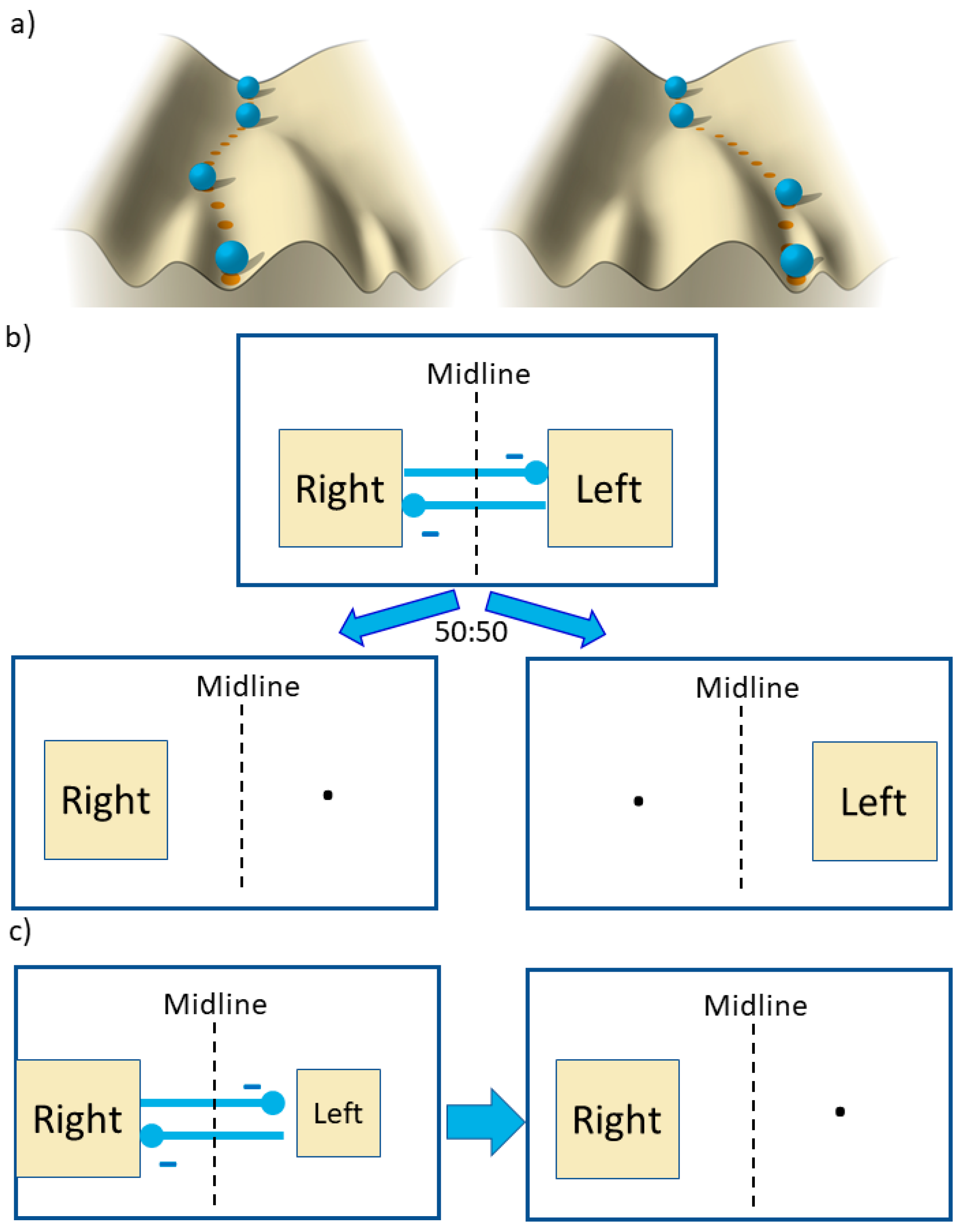
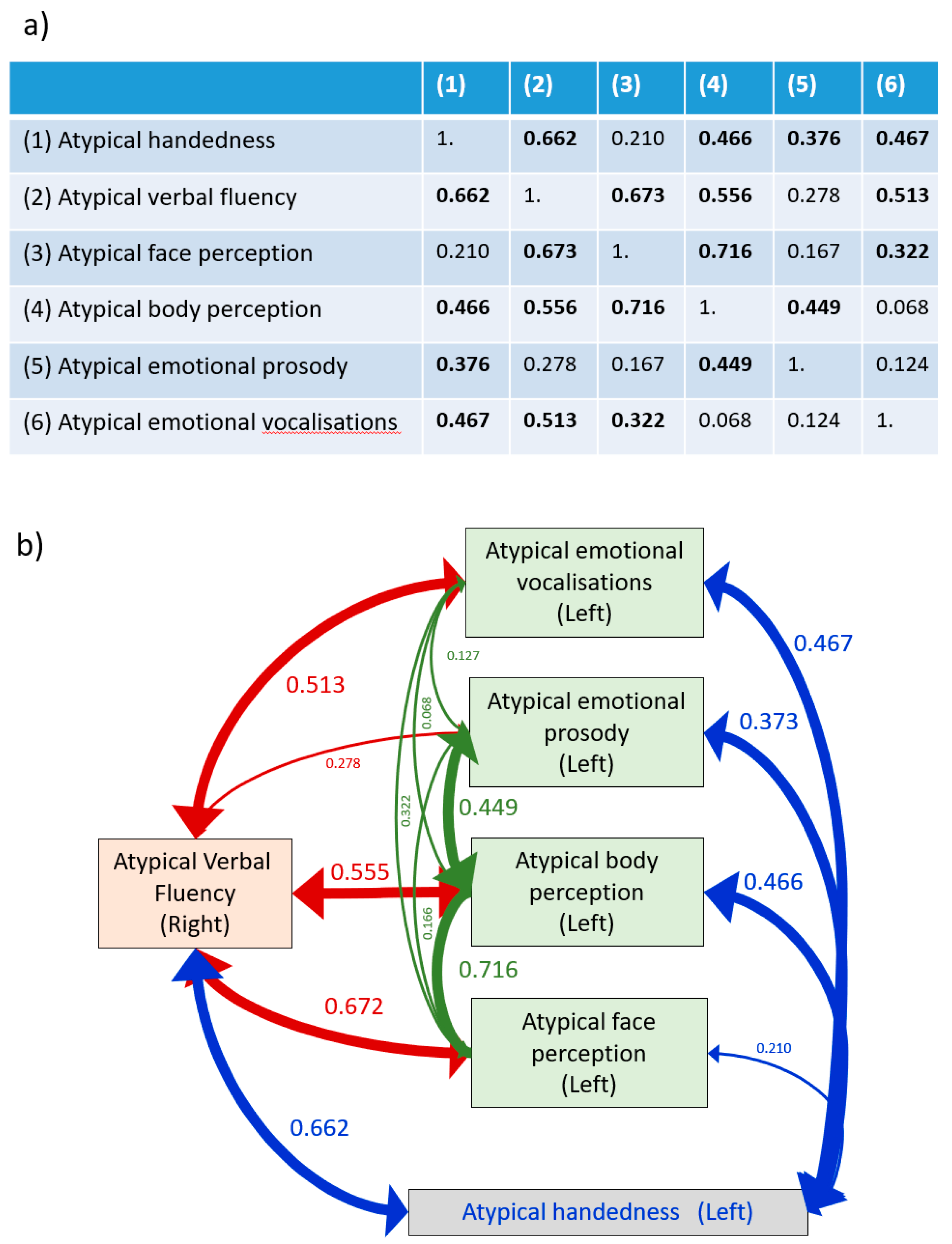
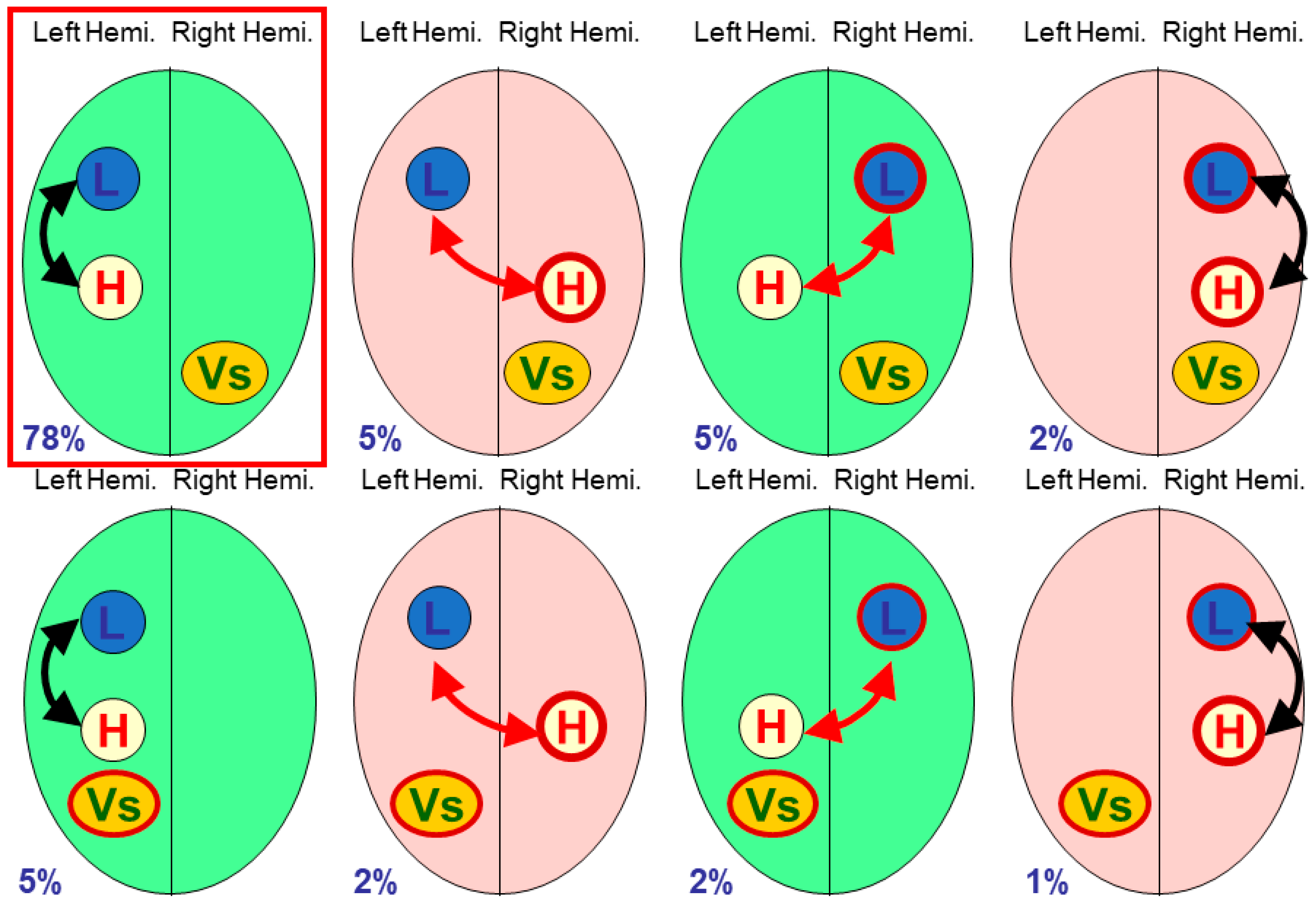
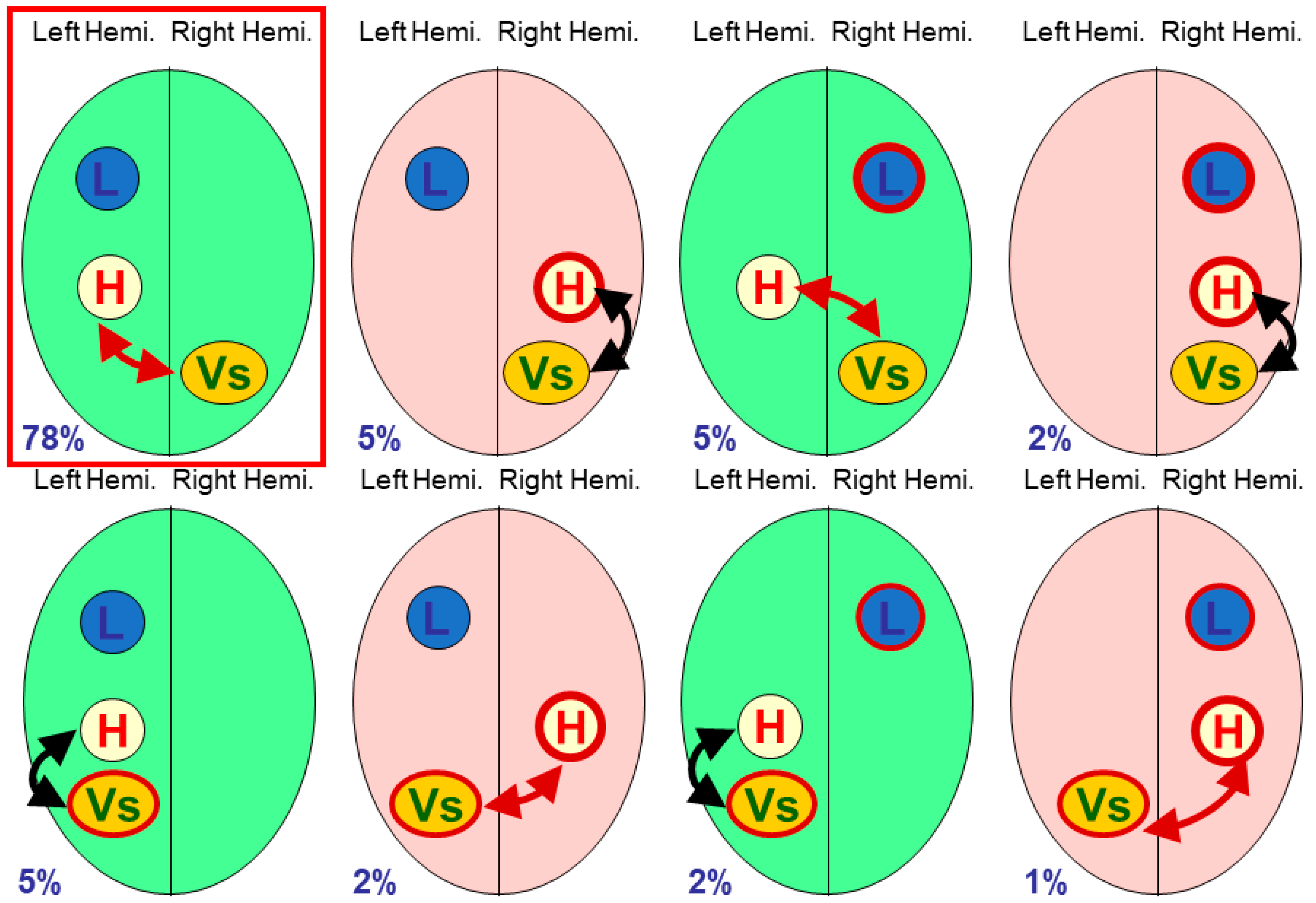
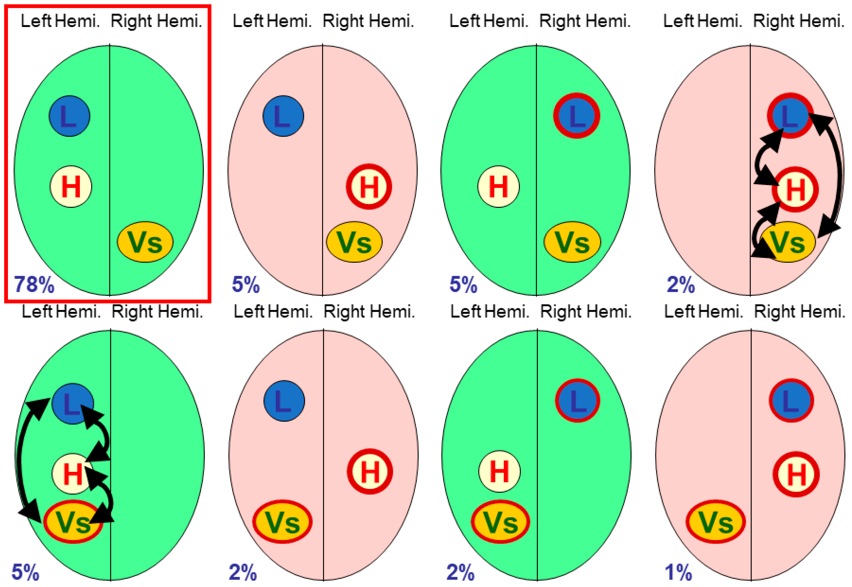
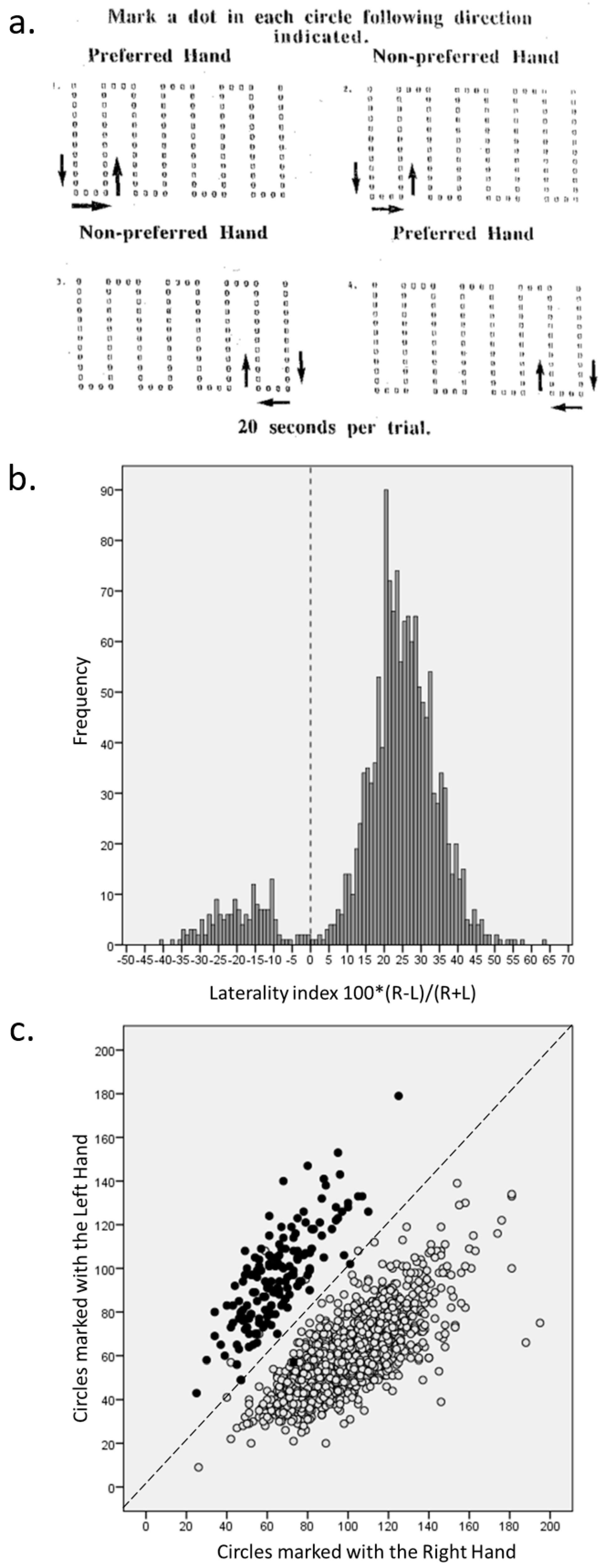
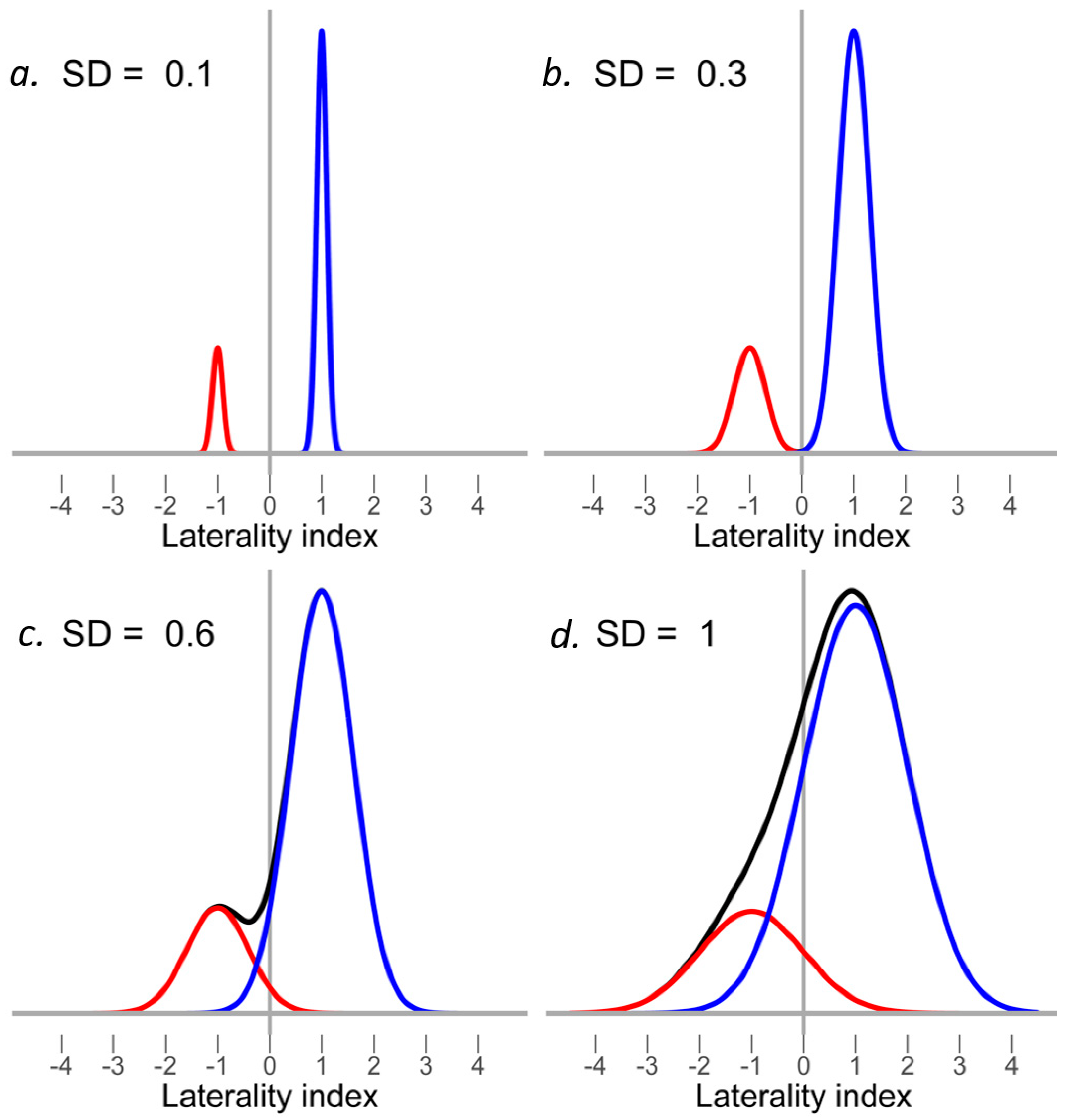
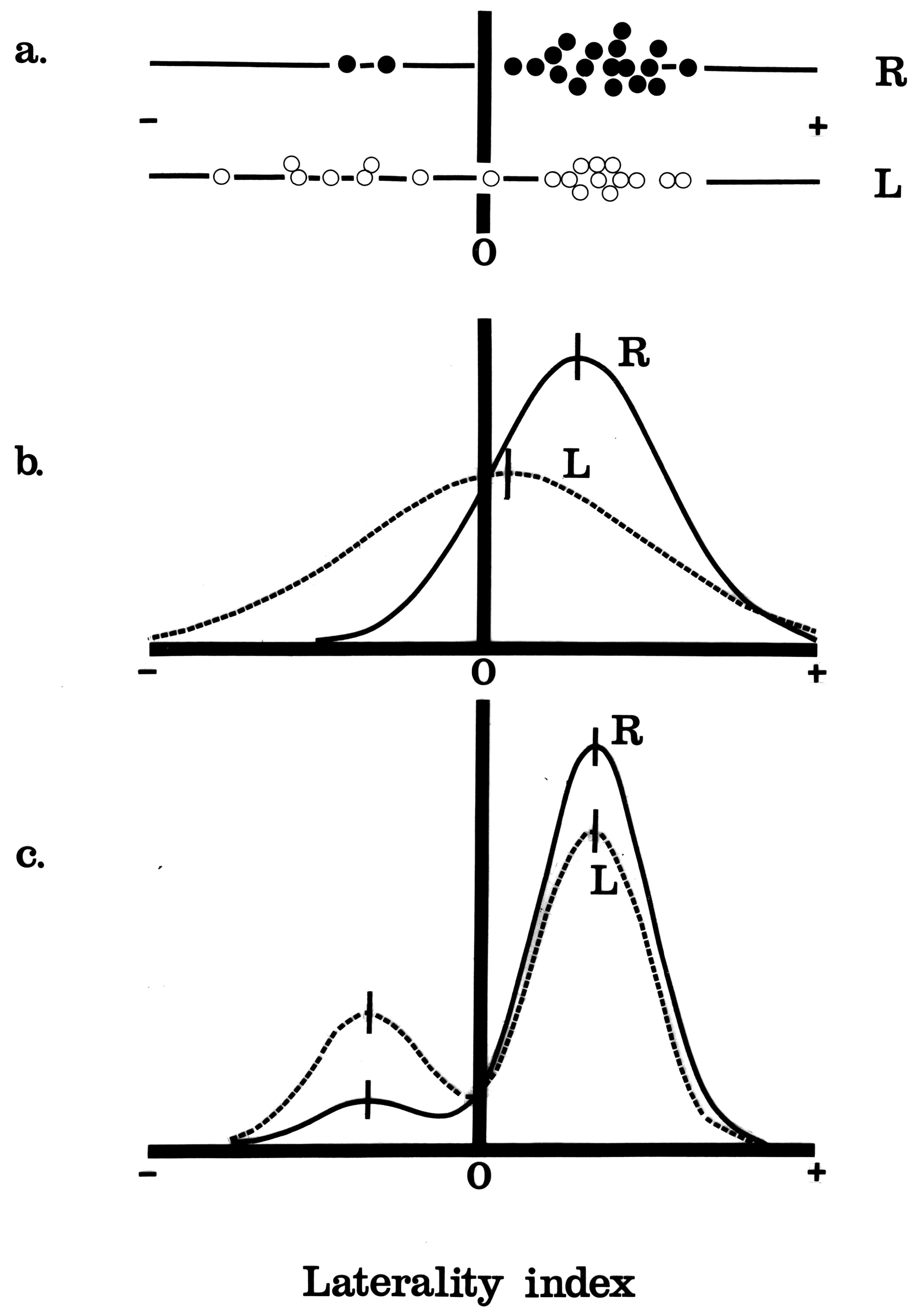
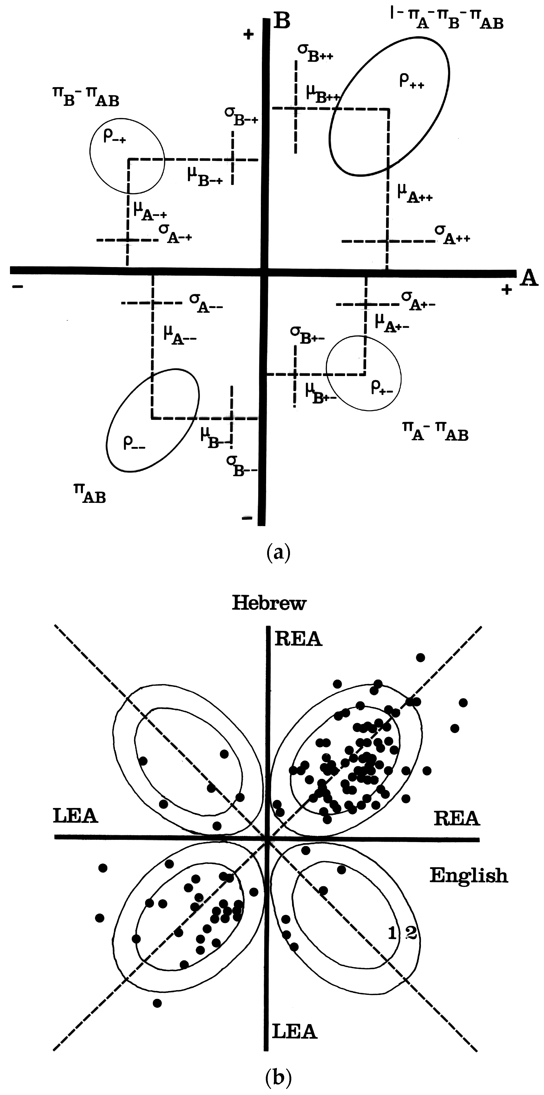
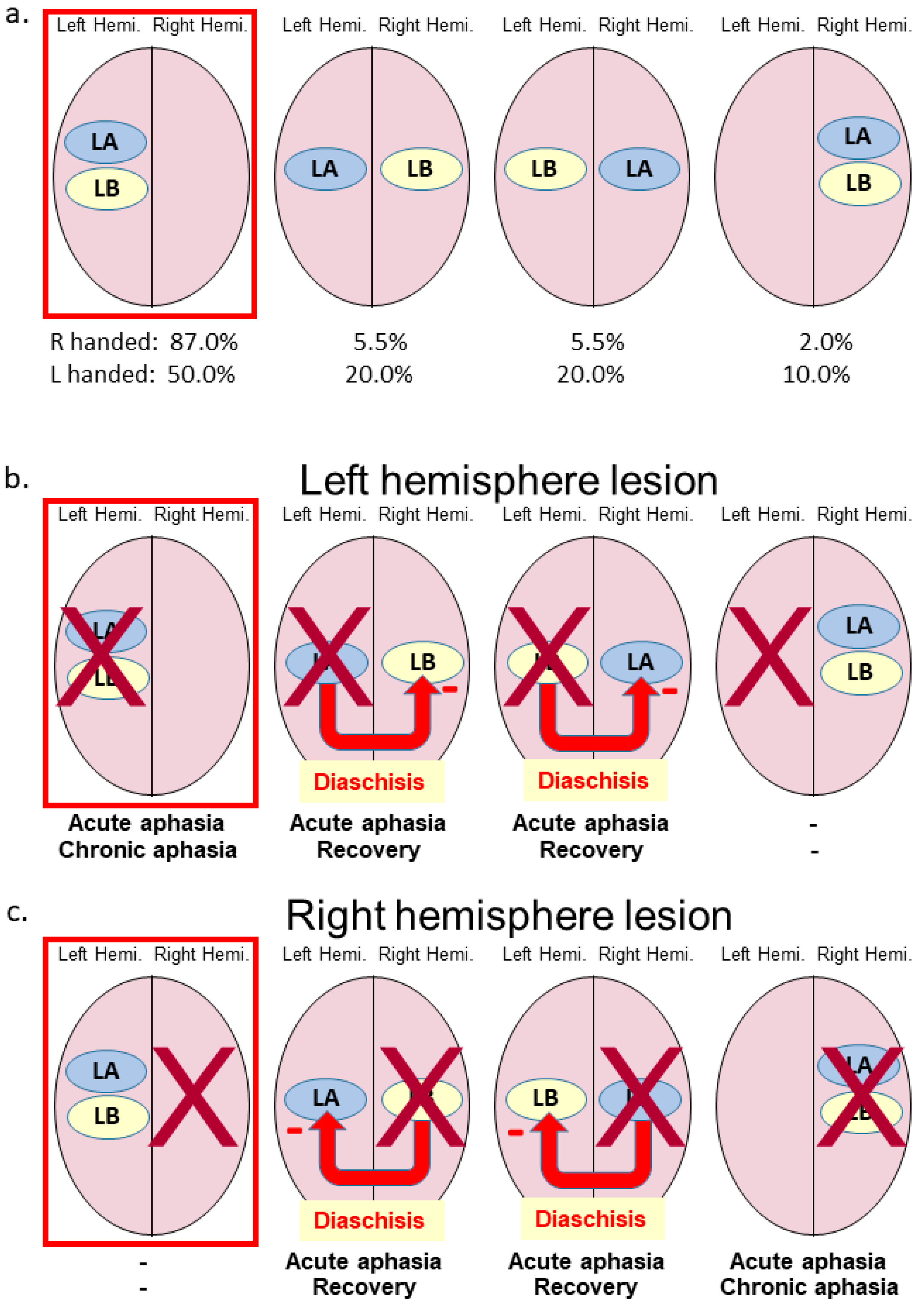
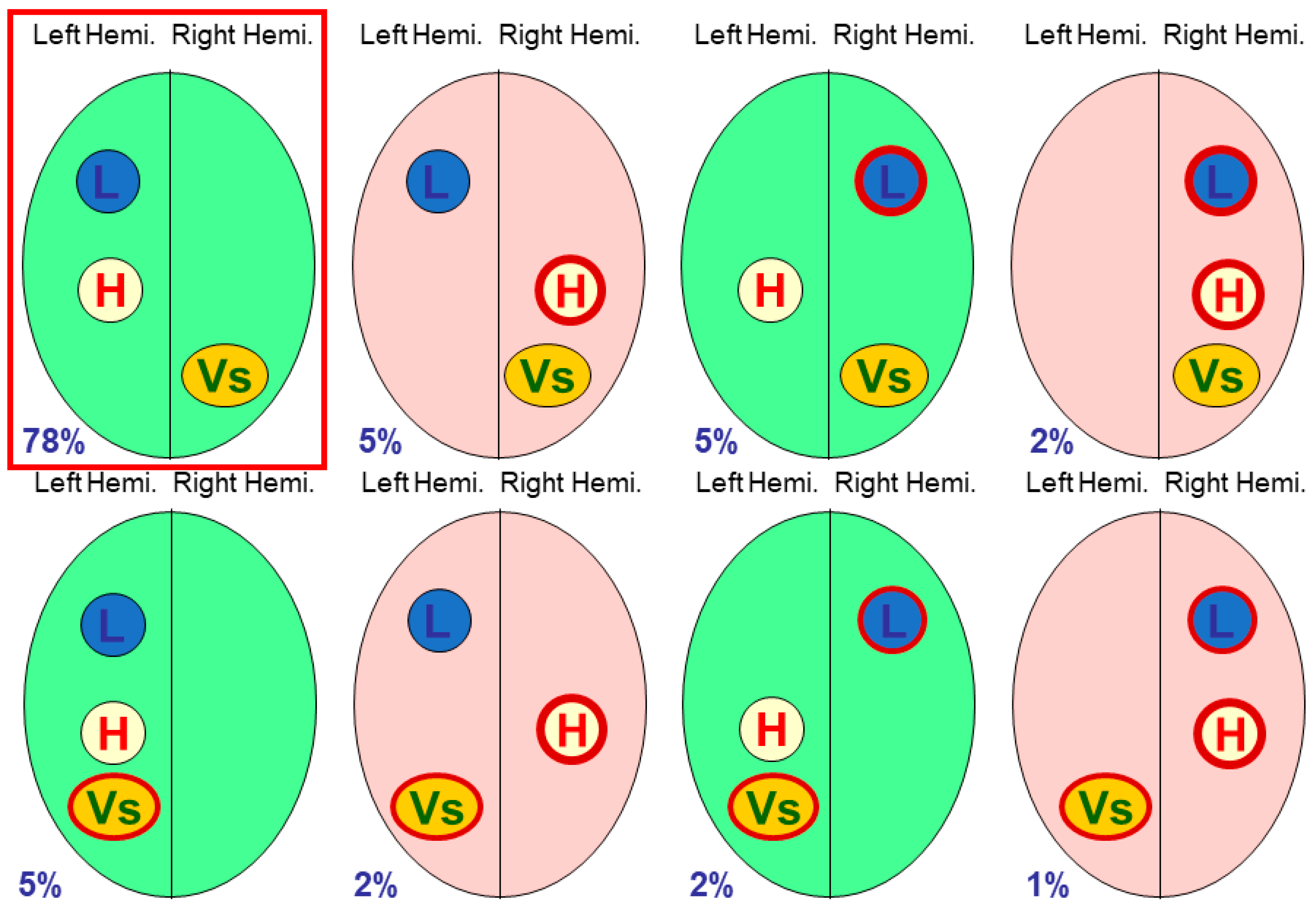
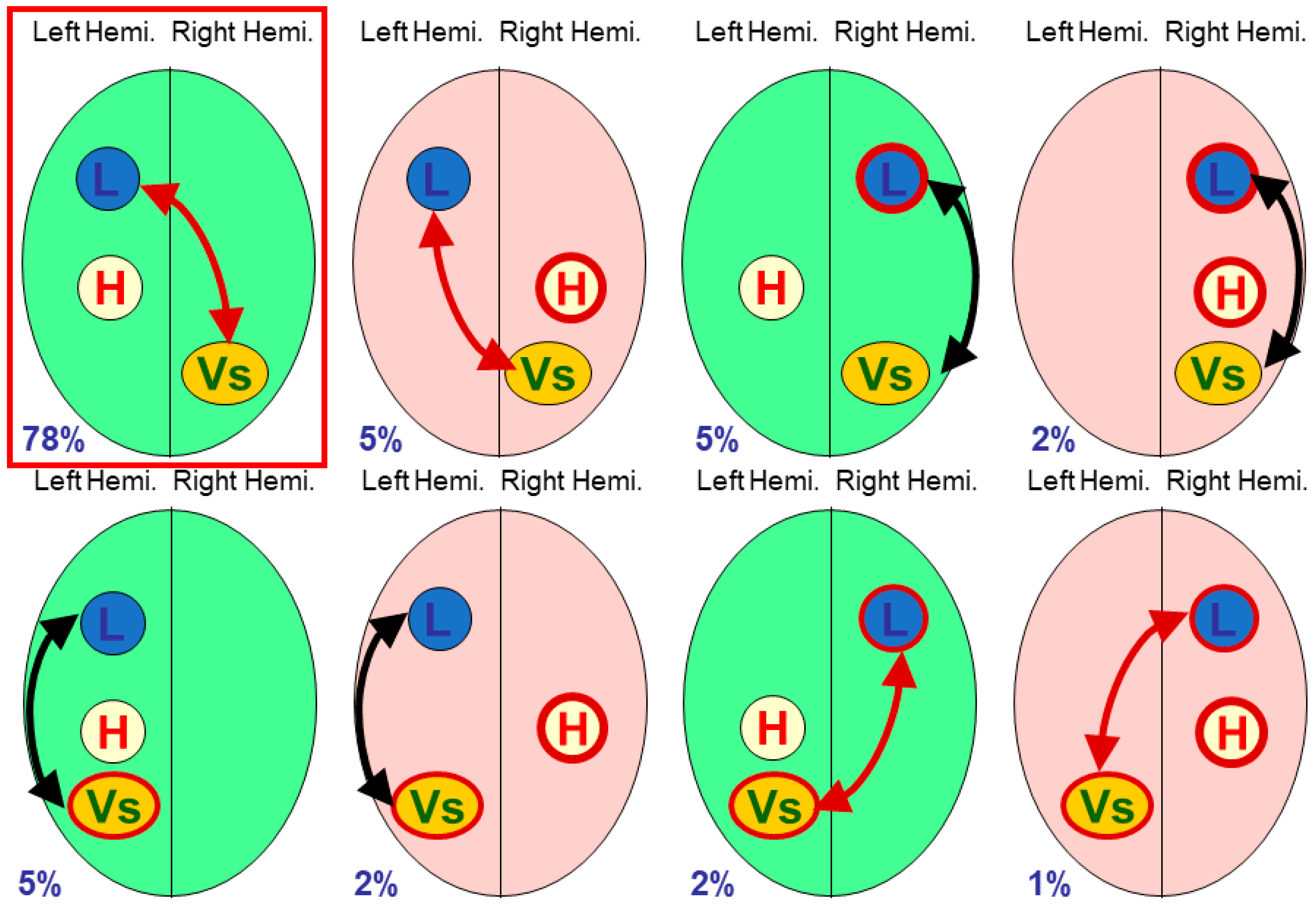