GPU-Accelerated Multi-Objective Optimal Planning in Stochastic Dynamic Environments

Abstract

The importance of autonomous marine vehicles is increasing in a wide range of ocean science and engineering applications. Multi-objective optimization, where trade-offs between multiple conflicting objectives are achieved (such as minimizing expected mission time, energy consumption, and environmental energy harvesting), is crucial for planning optimal routes in stochastic dynamic ocean environments. We develop a multi-objective path planner in stochastic dynamic flows by further developing and improving our recently developed end-to-end GPU-accelerated single-objective Markov Decision Process path planner. MDPs with scalarized rewards for multiple objectives are formulated and solved in idealized stochastic dynamic ocean environments with dynamic obstacles. Three simulated mission scenarios are completed to elucidate our approach and capabilities: (i) an agent moving from a start to target by minimizing travel time and net-energy consumption when harvesting solar energy in an uncertain flow; (ii) an agent moving from a start to target by minimizing travel time and-energy consumption with uncertainties in obstacle initial positions; (iii) an agent attempting to cross a shipping channel while avoiding multiple fast moving ships in an uncertain flow. Optimal operating curves are computed in a fraction of the time that would be required for existing solvers and algorithms. Crucially, our solution can serve as the benchmark for other approximate AI algorithms such as Reinforcement Learning and help improve explainability of those models.

1. Introduction

Optimal routing is essential for autonomous marine vehicles exploring the world’s oceans and assisting in scientific, commercial, and maritime security applications. In several situations, these vehicles are required to perform complex multi-objective missions in a stochastic and dynamic oceanic environment where they get significantly advected by the currents [1,2]. Recent work has utilized these flows for reducing operational costs in single-objective missions (either time- or energy-optimal) [3,4,5,6]. Optimal routing where an appropriate trade-off between multiple objectives is achieved is useful to improve operational efficiency and reduce costs. However, such simultaneous multi-objective planning, where travel time and net-energy (fuel) requirements are minimized in uncertain dynamic environments specified by stochastic forecasts from rigorous flow physics models has not been attempted yet. The challenge is primarily the computational cost (e.g., [7,8,9]). Existing Markov Decision Process (MDP) [4] or Reinforcement Learning [10,11] path planners are slow for realistic real-time applications. Path planners based on Dijkstra’s algorithm [12], variants of A${}^{*}$ [13,14] and Delayed D${}^{*}$ [15] work well in deterministic settings, but their Monte Carlo versions are computationally inefficient. [16] provides a survey of many such path planning algorithms. On the other hand, there are efficient level-set path planners [17,18] which have only been developed for single objective missions in stochastic environments and their extension requires further theoretical and methodological development.

Recently, we developed an end-to-end GPU accelerated MDP-based planner for single-objective missions of autonomous marine vehicles in stochastic dynamic flows [19]. The planner first builds the MDP model state transition probability and rewards. Next, it solves the built MDP efficiently using a GPU. Our single objective planner is based on two key ideas: (i) state transition probabilities and expected one-step rewards involve multiple independent computations that can be efficiently parallelized using a GPU, by writing new CUDA kernels specifically for this computation, and (ii) the state transition probability matrices (STMs) are sparse, allowing the use of efficient GPU-implemented libraries for sparse matrix operations. Multiple innovations in the implementation resulted in speed-ups of 600–1000× compared to conventional sequential methods. We also introduced more complicated planning environments with a stochastic dynamic scalar field and a stochastic dynamic flow field. The present paper further develops the above end-to-end GPU accelerated MDP-based optimal path planner to solve multi-objective planning problems.

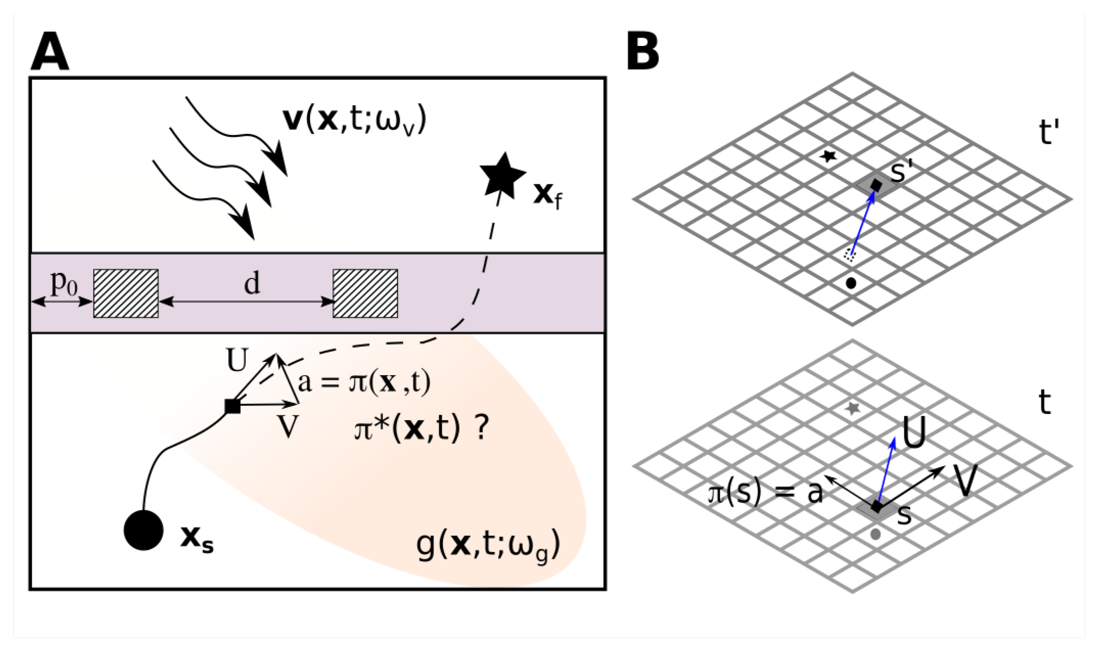
1.1. Problem Statement

Let $\mathbf{x}\in {\mathbb{R}}^n$ ($n=2,3$ for 2, 3-D space) denote space and $t\in [0,\infty )$ denote time of a spatio-temporal domain (Figure 1A) where an autonomous agent completes a mission by traveling from ${\mathbf{x}}_s$ at time $t=0$ to ${\mathbf{x}}_f$ in an manner that optimizes multiple objectives. Let $\mathbf{v}(\mathbf{x},t;{\omega }_v)$ be a stochastic, dynamic flow in the domain that strongly advects the agent. Further, let $g(\mathbf{x},t;{\omega }_g)$ be a stochastic dynamic scalar field (like solar, wind or wave energy) that the agent must collect during its mission. Here, ${\omega }_v$ and ${\omega }_g$ are samples of random variables ${\mathsf{\Omega }}_v$ and ${\mathsf{\Omega }}_g$ drawn from their respective probability distribution functions. Each sample ${\omega }_v$ and ${\omega }_g$ corresponds to a realization of the random velocity field and random scalar field, respectively. The agent maneuvers by performing an action a according to a deterministic policy $\pi$ and is simultaneously advected by the instantaneous velocity field $\mathbf{V}$. The agent must avoid dynamic obstacles along the way. For demonstration, we assume different configurations of obstacles (shown as striped rectangular boxes) for different applications. For example, in the first two applications (Section 4.1 and Section 4.2), we consider two such obstacles moving eastwards with the same speed and separated by a distance d. The x-coordinate of the obstacle on the left at time $t=0$ is $p_0$ (Figure 1A).

Our goal is to find a set of optimal policies that approximate the Pareto-optimal front to obtain an operating curve for competing objectives of minimizing the expected travel time and expected energy consumption or net-energy consumption. An end user can select any point from the operating curve that satisfies other operational requirements.

1.2. Prior Work

Multi-objective optimization [20,21,22] involves selecting the best solution from a Pareto-optimal front or operating curve using user-specified preferences that quantify the importance of conflicting objectives. If the preferences are known a-priori, the most common method used is the weighted sum method. Here, a linear sum of all the objectives is considered as a single objective and a solution is computed. For a-posteriori preference articulation, bio-inspired techniques such as genetic algorithms [23] and particle swarm optimization [24] have been proposed, which are heuristic-based methods and do not guarantee convergence to the optimal solution. Hence, these methods find limited applications in stochastic control applications.

Multi-objective MDPs (MOMDPs) formulate rewards as vectors instead of scalars, where each vector component is a separate independent objective. Ref. [25] discusses different classes of single-policy and multi-policy methods available to solve MOMDPs. A common single-policy approach is to convert the multi-objective reward vector into a scalarized value, making it possible to use existing methods to solve MDPs if weights are known apriori. Alternatively, Ref. [26] uses a nonlinear Tchebycheff function to scalarize the reward vector. Lexicographic MDPs [27] can be useful when a higher number of objectives are present and can be ordered in terms of significance (such as safety over cost and time, etc.). Constrained MDPs (CMDPs) optimize for a single objective with bounds for other objectives and various methods have been described in [28] to solve such problems. Ref. [29] discusses a dynamic programming based approach to formulate a multi-objective voyage optimization problem.

Another approach is to model the MOMDP as a partially observable MDP (POMDP) [30]. The unobserved state in the POMDP formulation is equivalent to the actual objective and the belief vector is equivalent to the MOMDP weight vector. GPU-based parallel implementations that use the Monte-Carlo Value Iteration algorithm to solve the continuous-state POMDPs have been proposed [31,32]. Approximate point-based methods [33,34,35] have also been implemented with GPUs to solve POMDPs [36]. Despite the available methods, solving MOMDPs and POMDPs remains computationally demanding and prohibitive for large-scale problems, especially for path planning of autonomous marine vehicles.

In [37], a linear combination of rewards is used to find the convex hull (a subset of Pareto front) by the Convex Hull Value Iteration algorithm. Multiple runs of a weighted sum method to get an approximate Pareto front or operating curve was proposed [20,25], but a single run itself was computationally infeasible for large scale applications. We propose using our recent GPU accelerated algorithm [19] to make this approach feasible.

The present paper’s key contributions are: (i) development and implementation of a computationally efficient GPU-accelerated algorithm to solve multi-objective optimal path planning problems in stochastic dynamic environments. We build an MDP model with a scalarized weighted sum reward function, compute optimal policies and operating curves in a fraction of the time required by traditional solvers, and (ii) demonstration of our algorithm for two applications in an idealized stochastic ocean flow environment, including a novel “shipping channel crossing” mission. Further, the uncertain environment flow is modeled using the dynamically orthogonal stochastic flow equations.

In what follows, we first briefly introduce the MDP framework for optimal planning (Section 2). Next, we develop our multi-objective optimal planner (Section 3). Then, we demonstrate its applications and highlight the computational advantages in Section 4. Finally, we conclude in Section 5.

2. Optimal Path Planning with MDPs

We use a finite horizon, undiscounted, total cost MDP defined by the tuple $\langle \mathcal{S},\mathcal{A},P,R\rangle$ to solve our problem statement. Here, $\mathcal{S}$ and $\mathcal{A}$ are the sets of states and actions, P is the state transition probabilities, and R is the expected one-step rewards. The computational domain is discretized to a spatio-temporal grid world (Figure 1B), where each discrete state (shown as a cell) s is indexed by discrete $({\mathbf{x}}_s,t_s)$. The random velocity at s is $\mathbf{v}(s;{\omega }_v)$. At each state s, the agent can take an action a. The spatial motion is given by ${\mathbf{x}}^{\prime }=f(\mathbf{x},a;{\omega }_v)=\mathbf{x}+(\mathbf{v}(s;{\omega }_v)+a)\Delta t$, and the temporal update is $t^{\prime }=t+\Delta t$. Such kinematic models are common in many practical applications [4,5,38,39,40,41,42], especially for autonomous marine vehicles where strong flows advect slow-moving agents. The successor state is defined as $s^{\prime }=cell({\mathbf{x}}^{\prime },t^{\prime })$, where the $cell\left(\right)$ function maps the spatial and temporal coordinates to the appropriate discrete state in the domain. Simultaneously, the agent also collects energy $g(s;{\omega }_g)$ and $g(s^{\prime };{\omega }_g)$ at s and $s^{\prime }$, respectively. The agent receives a one-step reward $R(s,a;s^{\prime })$ upon making the transition.The state transition probabilities and one-step rewards are $P_{s,s^{\prime }}^a=Pr(S_{t+1}=s^{\prime }|S_t=s,A_t=a)$ and $R(s,a)=\mathbb{E}\left[R_{t+1}\right|S_t=s,A_t=a]$. Here, $S_t,A_t,R_t$ are random variables that denote the state, action, and reward at time t, and $s,s^{\prime }\in \mathcal{S},a\in \mathcal{A}$. A policy $\pi$ is a mapping from the state space $\mathcal{S}$ to a probability distribution over the action space $\mathcal{A}$. An exact optimal policy ${\pi }^{*}\left(s\right)$$\forall s\in \mathcal{S}$ can be computed using the Bellman optimality conditions and dynamic programming as

$$\begin{array}{c}\hfill {\pi }^{*}\left(s\right)=\underset{a\in \mathcal{A}}{arg\; max}\left[R(s,a)+\sum _{s^{\prime }}{P}_{s,s^{\prime }}^a{v}^{*}\left(s^{\prime }\right)\right].\end{array}$$

(1)

For large state spaces corresponding to realistic problems without closed-form expression for flow uncertainty, computing the state transition matrices (STMs) and optimal policies is computationally infeasible. Hence, efficient and scalable algorithms are required. To this end, we recently developed an end-to-end GPU-accelerated planner [19] that computes these STMs and solves a single-objective MDP to obtain an optimal policy in a fraction of the time required by conventional sequential methods without resorting to approximate methods like Reinforcement Learning.

A forecast of the stochastic dynamic environmental flow field and energy field is required to compute the STMs and rewards for the MDP-based optimal planning problem. The stochastic flow field is obtained using the Dynamically Orthogonal (DO) barotropic Quasi-Geostrophic (QG) stochastic equations for canonical flows [17,18,43] and is decomposed in the form $\mathbf{v}(\mathbf{x},t;{\omega }_v)=\overline{\mathbf{v}}(\mathbf{x},t)+{\sum }_i{\mu }_i(t;{\omega }_v){\tilde{\mathbf{v}}}_i(\mathbf{x},t)$, where $\overline{\mathbf{v}}(\mathbf{x},t)$ is the so-called DO mean, ${\tilde{\mathbf{v}}}_i(\mathbf{x},t)$ are the DO modes, and ${\mu }_i(t;{\omega }_v)$ are the DO coefficients. The fluid flow data is obtained through the DO mean, modes, and coefficients, which are solved numerically using the computationally efficient stochastic DO Navier-Stokes equations [44,45,46].

The DO equations provide a significant computational advantage (100–10,000× speedup) over alternate techniques such as ensemble ocean forecasting to obtain the stochastic flow field [47]. Similarly, the energy field to be collected (e.g., solar, wind) must be obtained using appropriate environmental models [48,49]. The usage of flow simulations from the DO equations for the multi-objective planning missions is itself novel, and makes our approach stand apart from other path planning methods.

3. Multi-Objective Planning

Multi-objective problems can be converted into single objective problems using a suitable scalarization function [25,50]. Now, we formulate a weighted scalar reward function for our multi-objective path planning problem.

3.1. Multi-Objective Reward Formulation

The general reward structure for a single objective problem is as follows:

$$\begin{array}{c}\hfill \begin{array}{c}\hfill R_k(s,a;s^{\prime })=\left\{\begin{array}{cc}{r}_{term}\hfill & s^{\prime }\in {\mathcal{S}}_{targ}\hfill \\ r_{outbound}\hfill & s^{\prime }\in {\mathcal{S}}_{penalty}\hfill \\ R_{k,gen}(s,a;s^{\prime })\hfill & o.w.\hfill \end{array}\right.\end{array}\end{array}$$

(2)

Here, $k\in \{1,2,3\}$ and represents some mission objective. The agent is given a positive reward $r_{term}$ if it reaches a state in the set of target states ${\mathcal{S}}_{targ}$. This set contains all states corresponding to the target position $x_f$ at any timestep. The agent is penalized with a large negative reward $r_{outbound}$ if it reaches a state in the set of penalizable states ${\mathcal{S}}_{penalty}$. This set includes states that are outside the domain’s boundary, that coincide with a state occupied by an obstacle or states at the last time-step $N_t$. Therefore, the agent is penalized with $r_{outbound}$ if it lands in a state $s^{\prime }$ that is marked as an obstacle or if $s^{\prime }$ is not inside the spatial domain. It is also penalized if it cannot reach the target location until the last time-step $N_t$. This incentivizes the agent to avoid collision with obstacles and stay within the spatio-temporal domain. Otherwise, (i.e., if $s^{\prime }\in \mathcal{S}\setminus ({\mathcal{S}}_{targ}\bigcup {\mathcal{S}}_{penalty})$), the agent receives a general objective-specific one-step reward $R_{k,gen}(s,a;s^{\prime })$. It is to be noted that for a given $(s,a)$, $s^{\prime }$ depends on the random sample ${\omega }_v$.

For the multi-objective reward formulation, we consider problems that have two competing cost objectives. The first objective is to minimize expected travel time with the corresponding one-step reward

$$\begin{array}{c}\hfill R_{1,gen}(s,a;s^{\prime })=-\Delta t,\end{array}$$

(3)

i.e, the agent is penalized a constant value for each time-step. The second objective is to minimize either (i) Expected energy consumption with the one-step reward defined as

$$\begin{array}{c}\hfill R_{2,gen}(s,a;s^{\prime })=-c_f{F}^2\Delta t,\end{array}$$

(4)

or (ii) Expected net energy consumption with the one-step reward

$$\begin{array}{c}\hfill R_{3,gen}(s,a;s^{\prime })=\left[-c_f{F}^2+c_r\left(\frac{g\left(s\right)+g\left(s^{\prime }\right)}{2}\right)\right]\Delta t.\end{array}$$

(5)

In the former, the agent’s energy consumption is modeled as a function of its speed F ($c_f$ is a conversion constant). In the latter, the agent is equipped with an energy harvesting mechanism that collects from the stochastic dynamic energy field $g(•)$, and $c_r$ is a constant. The mission specific expected one-step reward is defined as

$$\begin{array}{c}\hfill R_k(s,a)=\mathbb{E}\left[R_k(s,a;s^{\prime })\right]k=\{1,2,3\},\end{array}$$

(6)

where the expectation is taken over the joint distribution $P(s^{\prime },{\omega }_g|s,a)$.

To solve a multi-objective problem, we first scalarize the one-step rewards by taking a linear combination of the rewards of the corresponding single-objective problems.

$$\begin{array}{c}\hfill R_{\alpha }(s,a)=(1-\alpha )R_m(s,a)+\alpha R_n(s,a)m,n\in \{1,2,3\}m\ne n.\end{array}$$

(7)

In the present paper, we consider two multi-objective problems. In one problem, we optimize the expected travel time and energy consumption. In the other, we optimize the expected travel time and net-energy consumption. The net energy consumption is the difference between the energy consumed by the agent’s propulsion for manoeuvring and the energy collected from the scalar energy (wind/solar) field. The scalarized one-step rewards for the two problems are defined as

$$\begin{array}{c}\hfill R_{{\alpha }_{12}}(s,a)=(1-{\alpha }_{12})R_1(s,a)+{\alpha }_{12}{R}_2(s,a),\end{array}$$

(8)

$$\begin{array}{c}\hfill R_{{\alpha }_{13}}(s,a)=(1-{\alpha }_{13})R_1(s,a)+{\alpha }_{13}{R}_3(s,a),\end{array}$$

(9)

where ${\alpha }_{12},{\alpha }_{13}$ are scalar weights. This is the weighted-sum approach to scalarization. Scalarization may also be done using other methods like an exponentially weighted product of objectives. We have experimented with the same and reported similar results (not shown here) without any improvement over the weighted-sum approach.

Then we compute the optimal value function for the problem by solving the Bellman optimality equation

$$\begin{array}{c}\hfill v_{\alpha }^{*}\left(s\right)=\underset{a\in \mathcal{A}}{max}\left[R_{\alpha }(s,a)+\sum _{s^{\prime }}{P}_{s,s^{\prime }}^a{v}_{\alpha }^{*}\left(s^{\prime }\right)\right],\end{array}$$

(10)

where α = α₁₂ or α = α₁₃, depending on the multi-objective problem. $v_{\alpha }^{*}$ is the optimal value function that maximizes the expected weighted sum of scalarized rewards R_α, given that the agent starts at a state s. $v_{\alpha }^{*}$ can be numerically computed using dynamic programming based algorithms like value iteration. Once $v_{\alpha }^{*}$ is obtained, we compute the corresponding optimal policy ${\pi }_{\alpha }^{*}$ using Equation (1).

3.2. GPU Accelerated Algorithm

Algorithm 1 shows an overview of our GPU accelerated planning algorithm implemented on CUDA [51]. There are two phases of the algorithm: (i) the initial model building phase (Lines 1–13); (ii) the reward scalarization and optimal policy computation phase (Line 14–17). The algorithm efficiently executes the first phase once and the second phase $n_{\alpha }$ number of $\alpha$ values in $[0,1]$ (Line 14). The algorithm takes as input the environment data and other problem specific parameters and returns a set of $n_{\alpha }$ optimal policies and value functions as output.

Let us consider solving the first multi-objective problem, where we optimize the expected travel time and energy consumption. In the initial model building phase, computing the STM $P^a$ and the expected one-step reward vectors $R_1^a,R_2^a$ corresponding to the two objectives (Line 10) requires $s^{\prime }\left({\omega }_v\right)$ and $R_k(s,a;s^{\prime }\left({\omega }_v\right))$, $k=\{1,2\}$, which are “embarrassingly parallel” computations that can be done simultaneously across states, actions, and realizations. However, limited GPU memory poses a challenge that we overcame by using the DO representation of the ocean flow and using sparse matrix formats for $P^a$. We also proved that using the mean of the scalar field is sufficient for the posed problem [19]. Moreover, Lines 5, 6, 8, and 9 inside the for-loops (Lines 3 and 4) correspond to efficient CUDA kernels that perform parallel computations for all states at time t and all realizations. For example, computing the STM $P^a$ for a given action a requires launching three CUDA kernels in sequence. Each kernel launches an optimal predetermined number of threads to perform a specific task in parallel. The first kernel (Line 5) computes $s^{\prime }\left({\omega }_v\right)$ and corresponding one-step rewards $R_1(s,a;s^{\prime }\left({\omega }_v\right))$ and $R_2(s,a;s^{\prime }\left({\omega }_v\right))$ for all realizations ${\omega }_v$, for all states at time t, in parallel, and stores them in an array. The next kernel (Line 6) accesses this array through multiple threads in parallel to count the number of times each $s^{\prime }$ is reached from the given $(s,a)$ across all realizations. Finally, another kernel (Line 8) reduces the count information to a structured STM $P^{a,t}$ in sparse format after memory is allocated for the same (Line 7). Similarly, another kernel (Line 9) is responsible for computing the mean of the one-step rewards across all realizations and the values are stored in the reward vectors $R_1^{a,t},R_2^{a,t}$. At the end of the loop the model for timestep t (i.e., $P^{a,t},R_1^{a,t},R_2^{a,t}$) is appended to that of the previous timestep. Consequently, after the last timestep we obtain $P^a,R_1^a,R_2^a\forall a\in \mathcal{A}$. Finally, all $P^a,R_1^a,R_2^a$ are appended across actions to obtain $\underline{P},\underline{R_1},\underline{R_2}$ (Line 13), which is necessary at a later stage for providing the appropriate input data structure to the sparse value iteration algorithm (Line 16). We refer the reader to the single objective version of the algorithm [19] for further details of the CUDA kernels and appending operations.

In the second phase, we compute the final model by scalarizing the expected one-step reward using a given $\alpha$ (Line 15). Thereafter, the optimal policy ${\pi }_{\alpha }^{*}$ is computed by plugging $\underline{P},\underline{R_{\alpha }}$ into a sparse value iteration algorithm (Line 16, [52]) with efficient parallel GPU-implementation of matrix operations. We obtain a set of optimal polices $\left\{{\pi }_{\alpha }^{*}\right\}$ by executing the second phase for $n_{\alpha }$ different values of $\alpha$. It must be noted that the initial model building phase is independent of $\alpha$ and is executed just once.

Algorithm 1: GPU Accelerated Planning Algorithm.

Input:$env\_data,prob\_type,prob\_params,grid\_params$

Output: {$v_{\alpha }^{*}$},{${\pi }_{\alpha }^{*}$}

1: Copy data to GPU;

2: Allocate GPU memory for intermediate data, $R_1^a$ and $R_2^a$ $\forall a$;

3: for ($t=0;t<N_t;t++$) do

4:  for $a\in \mathcal{A}$ do

5:   Compute $s^{\prime }\left({\omega }_v\right)$, $R_1(s,a;s^{\prime }\left({\omega }_v\right))$ and $R_2(s,a;s^{\prime }\left({\omega }_v\right))$ $\forall s\in S_t\forall {\omega }_v$;

6:   Count number of times $s^{\prime }$ is reached for given ($s, a$);

7:   Allocate memory for $P^{a,t}$;

8:   Reduce the count data to a sparse STM $P^{a,t}$;

9:   Compute $R_1(s,a):={\mathbb{E}}_{{\omega }_v}\left[R_1(s,a;s^{\prime }\left({\omega }_v\right))\right]$ and $R_2(s,a):={\mathbb{E}}_{{\omega }_v}\left[R_2(s,a;s^{\prime }\left({\omega }_v\right))\right]$ through sample mean and store in $R_1^{a,t}$, $R_2^{a,t}$;

10:   $P^a$, $R_1^a,R_2^a\leftarrow Append\_model\_in\_time(P^{a,t},R_1^{a,t},R_2^{a,t})$;

11:  end for

12: end for

13: $\underline{P},\underline{R_1},\underline{R_2}\leftarrow Append\_model\_in\_actions(\left\{P^a\right\},\left\{R_1^a\right\},\left\{R_2^a\right\})$;

14: for α in range ($0, 1, n^{\alpha }$) do

15:  Compute $\underline{R_{\alpha }}:=(1-\alpha )\underline{R_1}+\alpha \underline{R_2}$

16:  $v_{\alpha }^{*},{\pi }_{\alpha }^{*}\leftarrow Sparse\_Value\_Iter(\underline{P},\underline{R_{\alpha }})$;

17: end for

We achieve a 600–1000× reduction in the time required for the model building phase, depending on the GPU [19].

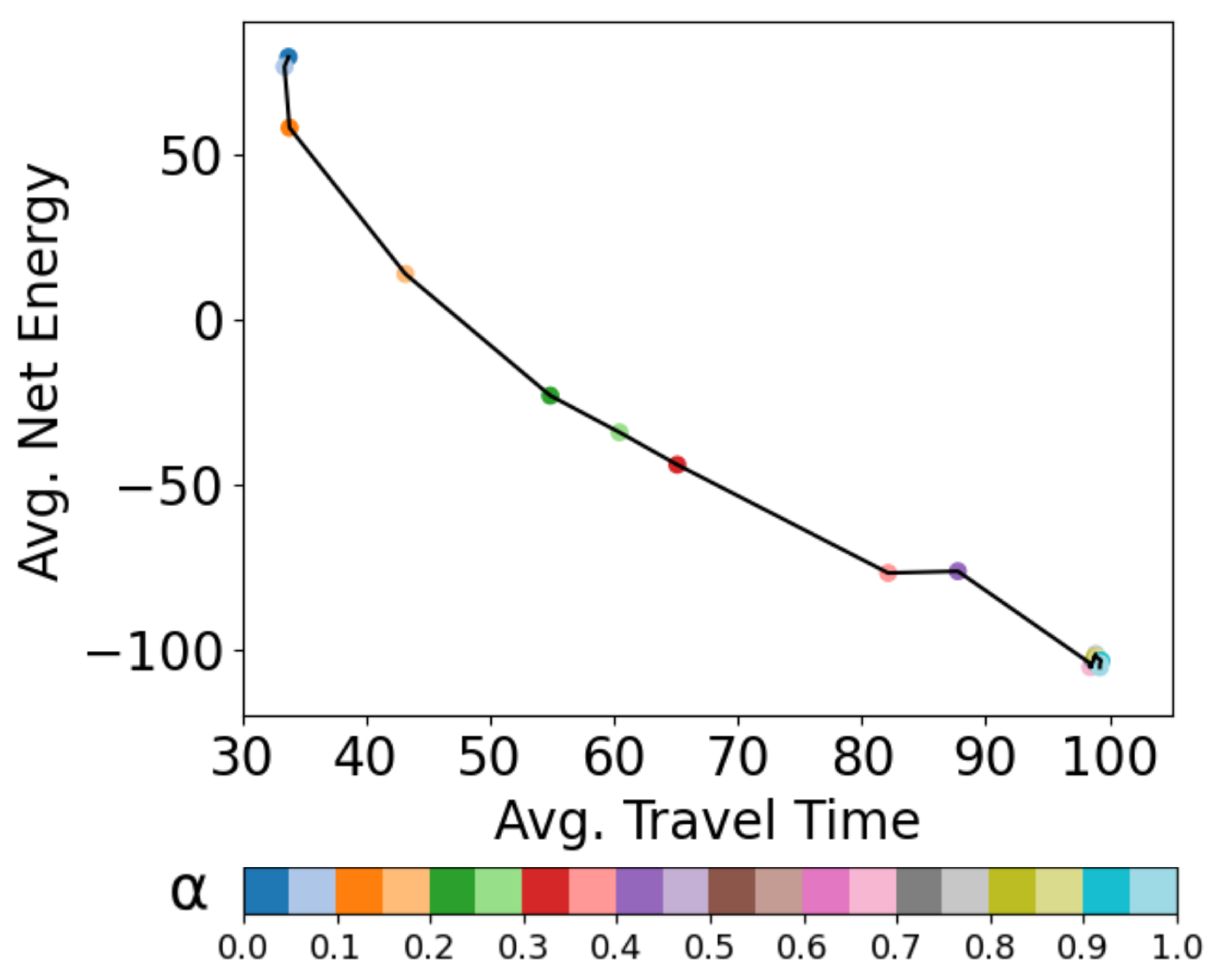
3.3. Operating Curves

For each $\alpha$, our algorithm computes the optimal policy ${\pi }_{\alpha }^{*}$. When $\alpha =0$, the optimal policy simply minimizes the expected travel time, whereas when $\alpha =1$ it minimizes the energy objective. Any other $\alpha \in (0,1)$ minimizes a weighted combination of the two.

The optimal operating curve is computed by executing the optimal policy ${\pi }_{\alpha }^{*}$ over all the realizations of the stochastic velocity field to obtain the average travel time $T_{avg}\left(\alpha \right)$ and energy (or net-energy) consumption $E_{avg}\left(\alpha \right)$ for each $\alpha$. An appropriate point can be chosen from the operating curve for field execution based on other operational requirements. In the following section, we demonstrate applications of our multi-objective planner.

4. Applications

We demonstrate two different multi-objective missions in a stochastic double-gyre ocean flow field obtained by solving the dynamically orthogonal quasi-geostrophic equations [44]. Such wind-driven double-gyre flows are encountered in several realistic scenarios in mid-latitude regional oceans such as the Northwest Atlantic ocean (Gulf Stream and eddies) [53,54]. See [17] for the equations and dynamics of this flow field that has been often used to demonstrate new methods for path planning. For easy reference, we have included the equations used to simulate the double-gyre flow field in Appendix B.

The planning is performed on a discrete spatio-temporal grid of size $100\times 100\times 120$, with $\Delta x=\Delta y=1$ and $\Delta t=1$ non-dimensional units. The environment and the dimensional scales are common for the first two applications, (Section 4.1 and Section 4.2) and are described next. The scales for the third application are different (see Section 4.3). For the first two applications, the non-dimensionalization is done such that one non-dimensional unit of space is 4 km and time is 0.115 days. Such state space dimensions are realistic [5,55] and have been chosen to demonstrate the computational capability of our algorithm with realistic grid dimensions. Note that for the algorithm developed in the present paper, the computational effort depends only on the grid size. Thus, it suffices to use an idealized flow field for demonstration.

Figure 2 shows the complete environment at $t=0$ for an example realization of the velocity field (Figure 2A) and the scalar energy field (Figure 2B). Both the fields are stochastic and dynamic (time-varying), but Figure 2 shows just one realization at $t=0$. The evolution of the environment with time can be seen in the backgrounds of Figure 3 and Figure 4 and also in the corresponding videos (

Table A1. Figures with trajectories and links to corresponding videos.

Figure Number	URL
Figure 3A	https://youtu.be/wn7VoLGuDl0, accessed on 4 April 2022
Figure 3B	https://youtu.be/9QTuTSBzg3Y, accessed on 4 April 2022
Figure 3C	https://youtu.be/Da4mIU691A8, accessed on 4 April 2022
Figure 4B	https://youtu.be/3V_GnrsOVaA, accessed on 4 April 2022
Figure 4C	https://youtu.be/hX6Qmm2WSJ4, accessed on 4 April 2022
Figure 7A	https://youtu.be/9bmKnY0LE5c, accessed on 4 April 2022
Figure 7B	https://youtu.be/MTUUQaHrxJc, accessed on 4 April 2022
Figure 7C	https://youtu.be/ZMv-31RTyvY, accessed on 4 April 2022

in Appendix A). The stochastic energy field g used for the energy collection objective is assumed to be a solar radiation incident on the ocean surface, simulating a cloud cover moving westwards (Figure 2B). The red region is a relatively sunny (high radiation) region whereas the yellow region is a relatively cloudy region (low radiation). An agent may spend time in the sunny regions of the domain to collect energy depending on its mission requirement. Further, the dynamic obstacles are assumed to be restricted zones that move eastwards with a known speed without affecting the flow. The starting positions of dynamic obstacles are assumed to be known in the first application ($p_0=10$) (Section 4.1) and as uncertain in the second application (Section 4.2). In non-dimensional units, the size of each obstacle is $10\times 10$ with $d=50$ and their speeds being $0.5$. The action space is discretized to 32 actions–16 possible headings, each with 2 possible magnitudes. It is to be noted that our planner can easily accommodate multiple vehicle speeds and headings, with different maximum speeds. These quantities are input parameters fed to the planner through a configuration file, which one can simply edit to simulate different vehicle speed capabilities. We highlight the same in Section 4.3 where we demonstrate the shipping channel crossing problem with two different agent capabilities; 5000 realizations of the flow field are considered. In dimensional units, the maximum magnitude of the flow field is 2.28 m/s (5.7 non-dimensional units), and the agent’s maximum speed is 0.8 m/s (2 non-dimensional units). These velocity magnitudes are derived from realistic flows and have been used for path planning applications [42]. Since the flow is relatively strong, the autonomous marine agent modeled here gets strongly advected. The agent’s mission is to start at $x_s=(40,15)$ (represented by a circular marker) to arrive at the position $x_f=(40,85)$ (represented by a star-shaped marker) while optimizing multiple-objectives.

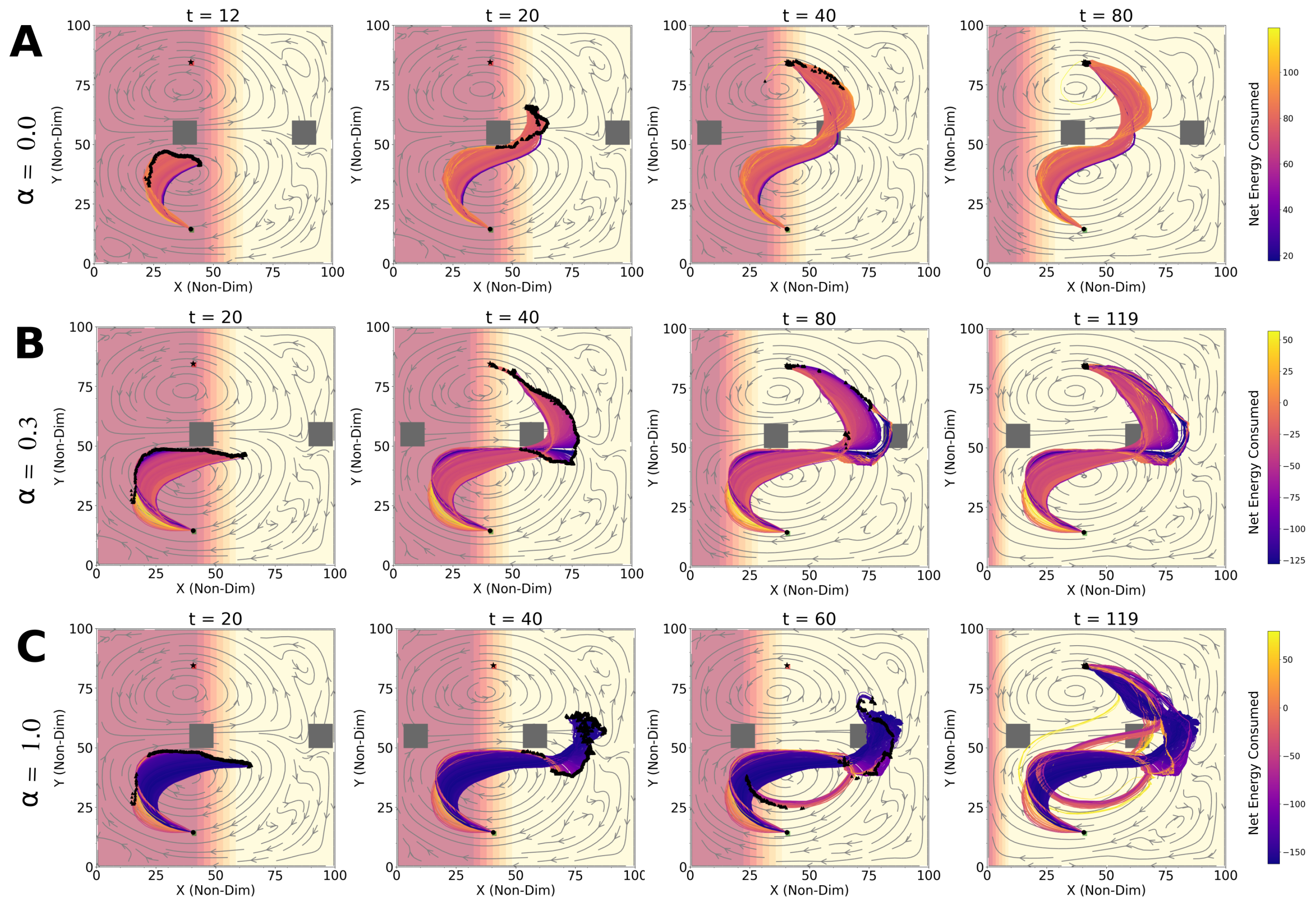
4.1. Optimal Time and Net Energy Missions

First, we consider a scenario where the agent must complete its mission while minimizing its expected travel time and net-energy consumption. We use the scalarized one-step rewards defined in Equation (9) for building and solving MDPs for multiple values of $\alpha \in [0,1]$ at intervals of $0.05$ with our GPU accelerated algorithm (Algorithm 1). We obtain the optimal operating curve (Figure 5) for expected time vs net-energy using the procedure defined in Section 3. Here, each point on the curve corresponds to a particular $\alpha$ value and shows the trade-off between the average mission travel time and net energy consumption for the corresponding optimal policy ${\pi }_{\alpha }^{*}$. Figure 3A–C show the temporal evolution of the trajectory distribution obtained by following the optimal policies for $\alpha =0$, $0.3$ and 1, respectively. For example, Figure 3A shows a distribution of trajectories that was obtained by following the optimal policy ${\pi }_{\alpha =0}^{*}$ across the 5000 realizations of the velocity field. Each trajectory is colored by the net-energy consumed by the agent in following it. The triangular marker at the end of each trajectory represents the position of the agent at the time (mentioned above each snapshot). As can be seen, the optimal policy and hence the trajectories for different $\alpha$ values have significantly different properties. When $\alpha =0$ (Figure 3A), the $R_{\alpha }$ is simply the same as $R_1(s,a)$ and ${\pi }_{\alpha =0}^{*}$ is a pure time-optimal policy. Therefore, the agent’s policy is to take high-speed actions while trying to utilize the flow to reach the target in the shortest possible time. Similarly, when $\alpha =1$ (Figure 3C), ${\pi }_{\alpha =1}^{*}$ is a pure net-energy optimal policy. Here, the agent takes low-speed actions and follows more time-consuming paths while utilizing the flow to expend less energy, thereby minimizing the net-energy consumption. In fact, for certain realizations, the agent loops around in the sunny region in the lower half of the domain. For these realizations, when the agent is in the region $X\in [50,70],Y\in [43,47]$ ($t=40$) the obstacle prevents the agent from moving up to the upper half of the domain. So instead of expending more energy to go against the flow to avoid the obstacle, it simply loops around in the lower half, utilizing the flow, collecting more energy from the radiation, and then proceeds towards the target unobstructed by the obstacle. For $\alpha =0.3$ (Figure 3B) the trajectories display an intermediate behavior between that of $\alpha =0$ and $\alpha =1$. Here, minimizing the net-energy consumption is prioritized just enough to make the agent take longer paths, but not enough to make loops in the sunny region as the agent also prioritizes its travel time to a certain extent. Please note that the timestamps of the snapshots in Figure 3A–C are different for better visualization of the evolving path distributions, but the radiation field is the same.

4.2. Optimal Time and Energy Missions with Unknown $p_0$

Second, we consider a mission where an Autonomous Underwater Vehicle (AUV) must reach its target $x_f$ while minimizing its expected travel time and energy consumption. However, in this case we assume that the initial position $p_0$ of the obstacle is unknown at $t=0$ (see Figure 1)) and model it as a uniform random variable. As our GPU-accelerated planner efficiently computes the optimal time-energy operating curve, the key idea now is to take samples of $p_0$ and obtain time-energy operating curves for each sample. In this application, the AUV is not collecting external energy as the focus is on time vs energy expenditure for an underwater application. Figure 4A shows the optimal time-energy operating curves for various values of $p_0$. Each plot along the row of Figure 4B shows the distribution of full trajectories obtained by following the optimal policy at $\alpha =0.3$ but for varying values of $p_0$. Figure 4C is similar to Figure 4B, but for $\alpha =0.7$. All plots along a column of Figure 4 correspond to the same $p_0$. The trajectories are colored by their energy consummations and the background is colored with the flow magnitude overlaid with streamlines. An interesting observation for $p_0=20$ and $p_0=30$ is that the operating curve has a U-shape, with the minima occurring at approximately $\alpha =0.3$. The part of the curve corresponding to $\alpha >0.3$ is not Pareto-optimal since the mission could be completed at a shorter travel time for some $\alpha <0.3$ with the same average energy consumption. For example, for $p_0=20$ in Figure 4A, the policies for $\alpha =0.25$ (light green dot) and $\alpha =0.55$ (light brown dot) consume nearly the same amount of average energy (70 units) but the average travel time for the former is nearly 10 units less compared to the latter. This makes the policy at $\alpha =0.55$ sub-optimal in the Pareto sense. A similar argument holds true for all policies with $\alpha >0.3$. The U-shape is a consequence of the following. As we increase $\alpha$, more weight is given to the energy objective, which results in the agent taking low-velocity actions, utilizing the flow and consuming less energy at the expense of more time. However, the relative velocities of the flow, the obstacles and the AUV are such that, for most realizations, the obstacle blocks the AUV’s path from the north as the AUV moves from west to east in the region $Y\in [40,50]$. As a result, the AUV has to maneuver and wait for the obstacle to move away (see the region $X\in [70,80],Y\in [40,50]$ in Figure 4C for $p_0=20$ and $p_0=30$). In contrast, for $\alpha =0.3,p_0=20$ (Figure 4B), the AUV easily maneuvers through the space between the two obstacles. This results in the AUV consuming more energy on average because of the delay caused by the obstacle. Another interesting observation is the apparently erratic behavior of the agent for some realizations (yellow colored trajectories) around the region $X\in [65,75],Y\in [55,65]$ in Figure 4B for $p_0=20$. The reason is that these realizations of the flow field have a larger southern gyre, and the said region experiences strong currents in the southern and south-eastern directions (see Figure A1 in Appendix A). On the other hand, the agent’s policy is to move in the opposite direction towards the target, hence resulting in small loops or sharp turns. Such loops in trajectories are typical of low-speed agents that get advected by eddies and gyres [3]. In real operations, we could analyze a series of time-energy operating curves to obtain the Pareto-optimal operating region (in this case $\alpha \in [0.1,0.3]$). Then, an AUV can be operated at a suitable operating point in this region as per other operational requirements.

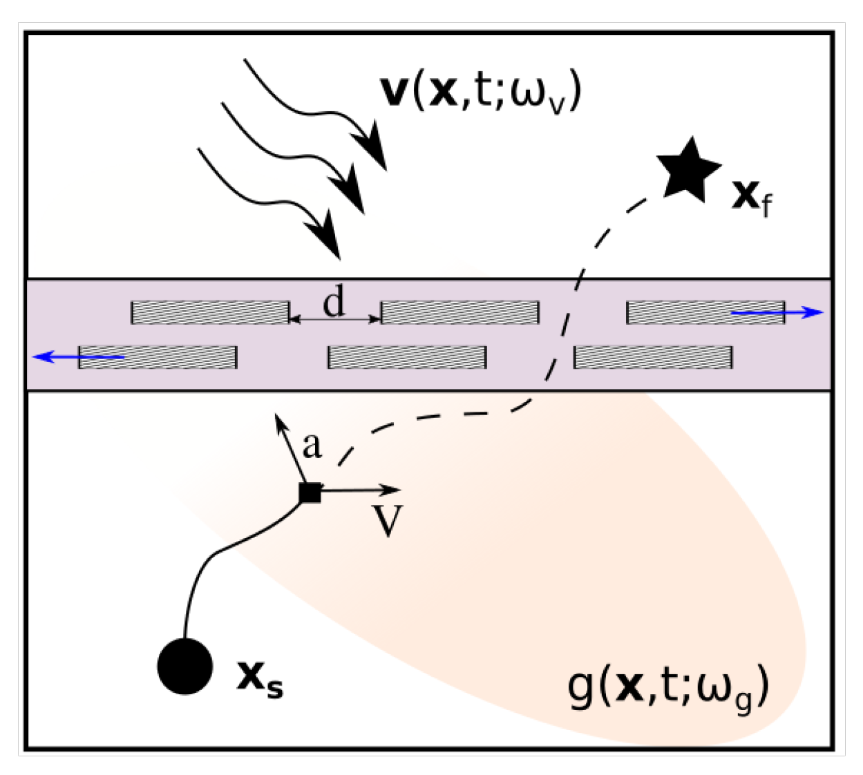
4.3. Shipping Channel Crossing Problem

Third, we demonstrate a shipping channel crossing problem. The shipping channel is the purple rectangular region in the domain, which is continuously used by ships to traverse across the grid (Figure 6). The agent must avoid possible collisions with these ships and safely cross the shipping channel to reach the target location while optimizing time and energy consumption. We consider a time-energy problem as the focus is on demonstration of our computational algorithm in a busy ship channel crossing application. However, we can just as easily consider scenarios where the agent also collects a scalar field along the way to optimize for its net-energy consumption. Here, the dynamic obstacles (shown in thin striped horizontal rectangles) represent two queues of ships continuously moving through the channel. Ships in the upper and lower queues move eastwards and westwards, respectively. While the size spatio-temporal grid is still $100\times 100\times 120$, the dimensional scales for this “shipping channel crossing” problem have been reduced to demonstrate the working of our planner in more complex and realistic scenarios. 1 non-dimensional unit of space is 50 m, and time is 30 s. The maximum speed of the AUV is considered to be 3 m/s, and the maximum flow velocity is 3 m/s (refer to Figure 2A for the spatial distribution of the flow speeds). The velocity of the ships is 8 m/s ($15.5$) knots, which is typical of large carrier ships. The shape of the obstacles (16 × 2 units) is also derived from typical carrier ship dimensions, which are 400 m × 50 m, and some buffer accounting for AUV safety and uncertainties in ship positions. The horizontal gap between two successive ships is $d=15$ units and remains constant. The distance between the two queues is eight units. The agent’s mission starts at $x_s=(40,15)$ and the target location is $x_f=(40,85)$.

Figure 7A–C show the temporal evolution of trajectory distributions that were obtained by executing the optimal policies for $\alpha =0$, $\alpha =0.4$ and $\alpha =1$, respectively. Here, the agent can move at two possible speeds—3 m/s or 1.5 m/s. Similar to the description in Section 4.1, when $\alpha =0$ (Figure 7A), the optimal policy is purely a time-optimal policy. Hence, the agent typically takes high-speed actions to reach the target location, consequently consuming more energy. When $\alpha =1$ (Figure 7C), the optimal policy is purely an energy-optimal policy, where the agent typically takes low-speed actions and utilizes the flow to reach the target location, resulting in more curved trajectories. When $\alpha =0.4$ (Figure 7B), the trajectories show an intermediate behavior as the optimal policy optimizes a weighted combination of both objectives. Please note that the timestamps of the snapshots for the three sub-figures are different for better visualization of the evolving path distributions, but the velocity field is the same.

A common feature of this application is that the agent efficiently utilizes the gaps in the queues of the ships to cross the shipping channel. Consequently, the trajectory distribution breaks into multiple thin bands based on the agent’s crossing these gaps across different realizations of the velocity field. The optimal policies also make the agent wait behind or move opposite a nearby ship to pass through the next possible gap quickly. This behavior can be observed in regions like $X\in [45,55],Y\in [45,48]$ in Figure 7B,C. We refer the reader to Table A1 in Appendix A for the videos of the same for better visualization.

We also demonstrate the shipping channel crossing problem with an agent capable of moving with three possible speeds—zero-speed, cruising speed (1.5 m/s), and maximum speed (3 m/s). Figure 8 shows a distribution of full trajectories for $\alpha =0$, $\alpha =0.4$, and $\alpha =1$ for this case. A noticeable difference can be seen for $\alpha =1$ (energy-optimal planning) when compared to Figure 7C due to the agent’s use of the zero-speed action to conserve energy for its minimization. We have assumed a known initial position of the queue of ships for this scenario for clarity and visualization. However, we can easily extend the problem to one with uncertain initial positions similar to our demonstration in Section 4.2 and analyze corresponding operating curves. Moreover, we note that extending the action space is a trivial task for our planner and requires a simple change in the configuration file.

4.4. Computational Efficiency

Our GPU-accelerated planner computes a set of optimal policies based on the forecast of the stochastic, dynamic velocity, and scalar fields as done in [4,10,19] in a fraction of the time compared to sequential MDP-based methods of similar problem sizes [4,38]. The above applications were run on a NVIDIA RTX 8000 GPU. The average total computation time for each value of $\alpha$ is around 1 min. Similar problems with a larger state space $200\times 200\times 200$ take an average total time of 4 min per MDP. This is orders of magnitude smaller than conventional solvers (e.g., [4]). Thus, we may compute an optimal operating curve within a few hours on a single GPU. Further, as the solution of each MDP is independent of the other, we may use multi-GPU systems to solve multiple MDPs in parallel and achieve an even smaller overall computation time. It is to be noted that though larger grid sizes lead to larger compute times, the speed-up compared to its sequential counterpart remains the same, as evident in Figure 8 of [19]. Moreover, using more complicated velocity or energy fields or complex-shaped obstacles does not affect the computational time or speed-up, as these are simply inputs to the planner in the form of matrices and independent of the algorithm. Another advantage is that multiple operating curves, as demonstrated in (Section 4.2), can be computed within a few hours. This allows us to update our environment model with the latest information on the velocity and scalar fields available up to the day of the mission itself. Consequently, it enables us to compute more accurate policies, which would be impossible using conventional sequential algorithms that could take weeks.

4.5. Discussion and Future Extension

Among the set of optimal policies computed by our planner, each policy offers a trade-off between the two objectives, which is visible in the optimal operating curve. The AUV operator must choose one of the policies for mission operation based on his needs and experience. The agent traverses the environment by executing the chosen optimal policy (open-loop control), without taking measurements from the environment. As part of our future work, we plan to extend the algorithm for onboard routing through periodic re-planning (closed-loop control), which would require measurements of the observed velocity field through sensors like ADCP and solar/wind sensors to measure the solar/wind field.

The focus of this work is on the methodological development of a fast and exact algorithm for efficient planning of multi-objective missions for a single agent. We plan to conduct experiments with a physical AUV(or USV) in the future, similar to our earlier experiments to test our previously developed level-set based solution [42]. It is to be noted that we can extend our proposed algorithm for multi-agent planning by (i) including the coordinates of all the robots in the MDP’s state definition, (ii) defining the reward function as per the mission requirements of the multi-robot system. However, the size of the state space increases exponentially with the number of robots, which require new CUDA kernels to be written and can be taken up as future work.

5. Conclusions

We developed a multi-objective planner for optimal path planning of autonomous agents in stochastic dynamic flows. The multi-objective problem was converted into a single-objective MDP by scalarizing the one-step rewards with the weight $\alpha$. We used our end-to-end GPU accelerated planner to efficiently build the MDP by computing the state transition probabilities, the expected scalarized one-step rewards and optimal policies for multiple values of $\alpha$. Then we obtained a time vs energy (or time vs net-energy) operating curve in a fraction of the time required to solve just one MDP by traditional solvers. We demonstrated three multi-objective problems. In the first, we minimize the expected travel time and net-energy consumption of a surface vehicle collecting solar energy. In the second, we minimize the travel time and energy consumption of an AUV while considering an unknown initial positions of the obstacles. In the third, we minimize the expected travel time and energy consumption of an AUV crossing a shipping channel. We demonstrate that our planner is capable of computing optimal operating curves quickly for large realistic grid sizes. This allows us to plan paths for AUVs in real-time to use the most recent environment forecast data. Even though we emphasized an idealized flow field scenario, the algorithm works with any complex flow fields and the compute time only depends on the grid size. For future work, we plan to use our multi-objective planner for more complex missions, pursuit-evasion games, and on-board routing. Our results can serve as a benchmark for POMDPs, MOMDPs, and RL algorithms (with or without GPU acceleration). They can also serve as a benchmark for heuristic-based algorithms like NSGA II for optimal planning in stochastic dynamic environments. A major issue of explainable AI is explaining why approximate and heuristic algorithms such as RL or NSGA II compute whatever paths they compute. Our results can serve as the solution those algorithms must achieve, thereby improving their explainability.

References

1. Sherman, J.; Davis, R.; Owens, W.; Valdes, J. The autonomous underwater glider “Spray”. IEEE J. Ocean. Eng. 2001, 26, 437–446. [Google Scholar] [CrossRef] [Green Version]
2. Bellingham, J.G.; Rajan, K. Robotics in remote and hostile environments. Science 2007, 318, 1098–1102. [Google Scholar] [CrossRef] [Green Version]
3. Subramani, D.N.; Haley, P.J., Jr.; Lermusiaux, P.F.J. Energy-optimal Path Planning in the Coastal Ocean. JGR Oceans 2017, 122, 3981–4003. [Google Scholar] [CrossRef]
4. Kularatne, D.; Hajieghrary, H.; Hsieh, M.A. Optimal Path Planning in Time-Varying Flows with Forecasting Uncertainties. In Proceedings of the 2018 IEEE International Conference on Robotics and Automation (ICRA), Brisbane, Australia, 21–25 May 2018; pp. 1–8. [Google Scholar]
5. Pereira, A.A.; Binney, J.; Hollinger, G.A.; Sukhatme, G.S. Risk-aware Path Planning for Autonomous Underwater Vehicles using Predictive Ocean Models. J. Field Robot. 2013, 30, 741–762. [Google Scholar] [CrossRef]
6. Lermusiaux, P.F.J.; Haley, P.J., Jr.; Jana, S.; Gupta, A.; Kulkarni, C.S.; Mirabito, C.; Ali, W.H.; Subramani, D.N.; Dutt, A.; Lin, J.; et al. Optimal Planning and Sampling Predictions for Autonomous and Lagrangian Platforms and Sensors in the Northern Arabian Sea. Oceanography 2017, 30, 172–185. [Google Scholar] [CrossRef] [Green Version]
7. Rathbun, D.; Kragelund, S.; Pongpunwattana, A.; Capozzi, B. An evolution based path planning algorithm for autonomous motion of a UAV through uncertain environments. In Proceedings of the 21st Digital Avionics Systems Conference, Irvine, CA, USA, 27–31 October 2002; Volume 2, pp. 8D2-1–8D2-12. [Google Scholar] [CrossRef]
8. Wang, T.; Le Maître, O.P.; Hoteit, I.; Knio, O.M. Path planning in uncertain flow fields using ensemble method. Ocean. Dyn. 2016, 66, 1231–1251. [Google Scholar] [CrossRef]
9. Kewlani, G.; Ishigami, G.; Iagnemma, K. Stochastic mobility-based path planning in uncertain environments. In Proceedings of the IEEE/RSJ International Conference on Intelligent Robots and Systems, St. Louis, MO, USA, 10–15 October 2009; pp. 1183–1189. [Google Scholar] [CrossRef]
10. Chowdhury, R.; Subramani, D.N. Physics-Driven Machine Learning for Time-Optimal Path Planning in Stochastic Dynamic Flows. In Proceedings of the International Conference on Dynamic Data Driven Application Systems, Boston, MA, USA, 2–4 October 2020; Springer: Cham, Switzerland, 2020; pp. 293–301. [Google Scholar]
11. Anderlini, E.; Parker, G.G.; Thomas, G. Docking Control of an Autonomous Underwater Vehicle Using Reinforcement Learning. Appl. Sci. 2019, 9, 3456. [Google Scholar] [CrossRef] [Green Version]
12. Singh, Y.; Sharma, S.; Sutton, R.; Hatton, D.; Khan, A. Feasibility study of a constrained Dijkstra approach for optimal path planning of an unmanned surface vehicle in a dynamic maritime environment. In Proceedings of the 2018 IEEE International Conference on Autonomous Robot Systems and Competitions (ICARSC), Torres Vedras, Portugal, 25–27 April 2018; pp. 117–122. [Google Scholar] [CrossRef] [Green Version]
13. Wang, Z.; Xiang, X. Improved Astar Algorithm for Path Planning of Marine Robot. In Proceedings of the 2018 37th Chinese Control Conference (CCC), Wuhan, China, 25–27 July 2018; pp. 5410–5414. [Google Scholar] [CrossRef]
14. Singh, Y.; Sharma, S.; Sutton, R.; Hatton, D.; Khan, A. A constrained A* approach towards optimal path planning for an unmanned surface vehicle in a maritime environment containing dynamic obstacles and ocean currents. Ocean Eng. 2018, 169, 187–201. [Google Scholar] [CrossRef] [Green Version]
15. Ferguson, D.; Stentz, A. The Delayed D* Algorithm for Efficient Path Replanning. In Proceedings of the 2005 IEEE International Conference on Robotics and Automation, Barcelona, Spain, 18–22 April 2005; pp. 2045–2050. [Google Scholar] [CrossRef]
16. Vagale, A.; Oucheikh, R.; Bye, R.T.; Osen, O.L.; Fossen, T.I. Path planning and collision avoidance for autonomous surface vehicles I: A review. J. Mar. Sci. Technol. 2021, 26, 1292–1306. [Google Scholar] [CrossRef]
17. Subramani, D.N.; Wei, Q.J.; Lermusiaux, P.F.J. Stochastic Time-Optimal Path-Planning in Uncertain, Strong, and Dynamic Flows. Comp. Methods Appl. Mech. Eng. 2018, 333, 218–237. [Google Scholar] [CrossRef]
18. Subramani, D.N.; Lermusiaux, P.F.J. Energy-optimal Path Planning by Stochastic Dynamically Orthogonal Level-Set Optimization. Ocean. Model. 2016, 100, 57–77. [Google Scholar] [CrossRef] [Green Version]
19. Chowdhury, R.; Subramani, D. Optimal Path Planning of Autonomous Marine Vehicles in Stochastic Dynamic Ocean Flows using a GPU-Accelerated Algorithm. arXiv 2021, arXiv:2109.00857. [Google Scholar]
20. Andersson, J. A Survey of Multiobjective Optimization in Engineering Design; Department of Mechanical Engineering, Linktjping University: Linköping, Sweden, 2000. [Google Scholar]
21. Marler, R.T.; Arora, J.S. Survey of multi-objective optimization methods for engineering. Struct. Multidiscip. Optim. 2004, 26, 369–395. [Google Scholar] [CrossRef]
22. Stewart, R.H.; Palmer, T.S.; DuPont, B. A survey of multi-objective optimization methods and their applications for nuclear scientists and engineers. Prog. Nucl. Energy 2021, 138, 103830. [Google Scholar] [CrossRef]
23. Deb, K.; Pratap, A.; Agarwal, S.; Meyarivan, T. A fast and elitist multiobjective genetic algorithm: NSGA-II. IEEE Trans. Evol. Comput. 2002, 6, 182–197. [Google Scholar] [CrossRef] [Green Version]
24. Brownlee, J. Clever Algorithms: Nature-Inspired Programming Recipes; Lulu Press: Morrisville, NC, USA, 2011. [Google Scholar]
25. Roijers, D.M.; Vamplew, P.; Whiteson, S.; Dazeley, R. A survey of multi-objective sequential decision-making. J. Artif. Intell. Res. 2013, 48, 67–113. [Google Scholar] [CrossRef] [Green Version]
26. Perny, P.; Weng, P. On finding compromise solutions in multiobjective Markov decision processes. In ECAI 2010; IOS Press: Amsterdam, The Netherlands, 2010; pp. 969–970. [Google Scholar]
27. Wray, K.H.; Zilberstein, S.; Mouaddib, A.I. Multi-objective MDPs with conditional lexicographic reward preferences. In Proceedings of the Twenty-Ninth AAAI Conference on Artificial Intelligence, Austin, TX, USA, 25–30 January 2015. [Google Scholar]
28. Geibel, P. Reinforcement learning for MDPs with constraints. In Proceedings of the European Conference on Machine Learning, Berlin, Germany, 18–22 September 2006; Springer: Berlin/Heidelberg, Germany, 2006; pp. 646–653. [Google Scholar]
29. Zaccone, R.; Ottaviani, E.; Figari, M.; Altosole, M. Ship voyage optimization for safe and energy-efficient navigation: A dynamic programming approach. Ocean. Eng. 2018, 153, 215–224. [Google Scholar] [CrossRef]
30. White, C.C.; Kim, K.W. Solution procedures for vector criterion Markov Decision Processes. Large Scale Syst. 1980, 1, 129–140. [Google Scholar]
31. Lee, T.; Kim, Y.J. GPU-based motion planning under uncertainties using POMDP. In Proceedings of the 2013 IEEE International Conference on Robotics and Automation, Karlsruhe, Germany, 6–10 May 2013; pp. 4576–4581. [Google Scholar]
32. Lee, T.; Kim, Y.J. Massively parallel motion planning algorithms under uncertainty using POMDP. Int. J. Robot. Res. 2016, 35, 928–942. [Google Scholar] [CrossRef]
33. Spaan, M.T.; Vlassis, N. Perseus: Randomized point-based value iteration for POMDPs. J. Artif. Intell. Res. 2005, 24, 195–220. [Google Scholar] [CrossRef]
34. Pineau, J.; Gordon, G.; Thrun, S. Anytime point-based approximations for large POMDPs. J. Artif. Intell. Res. 2006, 27, 335–380. [Google Scholar] [CrossRef]
35. Shani, G.; Pineau, J.; Kaplow, R. A survey of point-based POMDP solvers. Auton. Agents Multi-Agent Syst. 2013, 27, 1–51. [Google Scholar] [CrossRef]
36. Wray, K.H.; Zilberstein, S. A parallel point-based POMDP algorithm leveraging GPUs. In Proceedings of the 2015 AAAI Fall Symposium Series, Arlington, VA, USA, 12–14 November 2015. [Google Scholar]
37. Barrett, L.; Narayanan, S. Learning all optimal policies with multiple criteria. In Proceedings of the 25th International Conference on Machine Learning, Helsinki, Finland, 5–9 July 2008; pp. 41–47. [Google Scholar]
38. Rao, D.; Williams, S.B. Large-scale path planning for underwater gliders in ocean currents. In Proceedings of the Australasian Conference on Robotics and Automation (ACRA), Sydney, Australia, 2–4 December 2009; pp. 2–4. [Google Scholar]
39. Fernández-Perdomo, E.; Cabrera-Gámez, J.; Hernández-Sosa, D.; Isern-González, J.; Domínguez-Brito, A.C.; Redondo, A.; Coca, J.; Ramos, A.G.; Fanjul, E.Á.; García, M. Path planning for gliders using Regional Ocean Models: Application of Pinzón path planner with the ESEOAT model and the RU27 trans-Atlantic flight data. In Proceedings of the OCEANS’10 IEEE SYDNEY, Sydney, Australia, 24–27 May 2010; pp. 1–10. [Google Scholar]
40. Smith, R.N.; Chao, Y.; Li, P.P.; Caron, D.A.; Jones, B.H.; Sukhatme, G.S. Planning and implementing trajectories for autonomous underwater vehicles to track evolving ocean processes based on predictions from a regional ocean model. Int. J. Robot. Res. 2010, 29, 1475–1497. [Google Scholar] [CrossRef] [Green Version]
41. Al-Sabban, W.H.; Gonzalez, L.F.; Smith, R.N. Wind-energy based path planning for unmanned aerial vehicles using markov decision processes. In Proceedings of the 2013 IEEE International Conference on Robotics and Automation, Karlsruhe, Germany, 6–10 May 2013; pp. 784–789. [Google Scholar]
42. Subramani, D.N.; Lermusiaux, P.F.J.; Haley, P.J., Jr.; Mirabito, C.; Jana, S.; Kulkarni, C.S.; Girard, A.; Wickman, D.; Edwards, J.; Smith, J. Time-Optimal Path Planning: Real-Time Sea Exercises. In Proceedings of the Oceans ’17 MTS/IEEE Conference, Aberdeen, UK, 19–22 June 2017. [Google Scholar] [CrossRef]
43. Lolla, T.; Lermusiaux, P.F.J.; Ueckermann, M.P.; Haley, P.J., Jr. Time-Optimal Path Planning in Dynamic Flows using Level Set Equations: Theory and Schemes. Ocean. Dyn. 2014, 64, 1373–1397. [Google Scholar] [CrossRef] [Green Version]
44. Sapsis, T.P.; Lermusiaux, P.F.J. Dynamically orthogonal field equations for continuous stochastic dynamical systems. Phys. D Nonlinear Phenom. 2009, 238, 2347–2360. [Google Scholar] [CrossRef]
45. Ueckermann, M.P.; Lermusiaux, P.F.J.; Sapsis, T.P. Numerical schemes for dynamically orthogonal equations of stochastic fluid and ocean flows. J. Comput. Phys. 2013, 233, 272–294. [Google Scholar] [CrossRef] [Green Version]
46. Subramani, D.N.; Lermusiaux, P.F.J. Risk-Optimal Path Planning in Stochastic Dynamic Environments. Comp. Methods Appl. Mech. Eng. 2019, 353, 391–415. [Google Scholar] [CrossRef]
47. Lermusiaux, P.F.J.; Subramani, D.N.; Lin, J.; Kulkarni, C.S.; Gupta, A.; Dutt, A.; Lolla, T.; Haley, P.J., Jr.; Ali, W.H.; Mirabito, C.; et al. A Future for Intelligent Autonomous Ocean Observing Systems. J. Mar. Res. 2017, 75, 765–813. [Google Scholar] [CrossRef]
48. Skamarock, W.; Klemp, J.; Dudhia, J.; Gill, D.; Liu, Z.; Berner, J.; Wang, W.; Powers, J.; Duda, M.; Barker, D.; et al. A Description of the Advanced Research WRF Model Version 4; Technical Report; National Center for Atmospheric Research: Boulder, CO, USA, 2019. [Google Scholar]
49. Tolman, H. User Manual and System Documentation of WAVEWATCH III TM Version 3.14; Technical Report; MMAB: College Park, MD, USA, 2009. [Google Scholar]
50. Sutton, R.S.; Barto, A.G. Reinforcement Learning: An Introduction; MIT Press: Cambridge, MA, USA, 2018. [Google Scholar]
51. NVIDIA; Vingelmann, P.; Fitzek, F.H. CUDA, Release: 10.2.89, 2020. Available online: https://developer.nvidia.com/cuda-toolkit (accessed on 1 February 2022).
52. Sapio, A.; Bhattacharyya, S.S.; Wolf, M. Efficient solving of Markov decision processes on GPUs using parallelized sparse matrices. In Proceedings of the 2018 Conference on Design and Architectures for Signal and Image Processing (DASIP), Porto, Portugal, 10–12 October 2018; pp. 13–18. [Google Scholar]
53. Gangopadhyay, A. Introduction to Ocean Circulation and Modeling; CRC Press: Boca Raton, FL, USA, 2022. [Google Scholar]
54. Cushman-Roisin, B.; Beckers, J.M. Introduction to Geophysical Fluid Dynamics: Physical and Numerical Aspects; Academic Press: Cambridge, MA, USA, 2011. [Google Scholar]
55. Podder, T.K.; Sibenac, M.; Bellingham, J.G. Applications and Challenges of AUV Docking Systems Deployed for Long-Term Science Missions; Monterey Bay Aquarium Research Institute: Moss Landing, CA, USA, 2019. [Google Scholar]
Figure 1. Schematic of the problem statement in continuous and discrete settings: (A) The autonomous agent’s mission is to travel from x s to x f in a domain under the influence of a stochastic dynamic flow field v ( x , t ; ω v ) and a stochastic dynamic scalar field g ( x , t ; ω g ) that must be collected. We seek a set of optimal policies π * ( x , t ) that optimizes a multi-objective cost function. (B) In the discretized spatio-temporal grid, the agent takes an action a = π ( s ) from state s at discrete time t to reach s in the next time-step t under the influence of random discrete velocity V ( s ) .
Jmse 10 00533 g001
Figure 2. Mission Environment (A) An example realization at t = 0 of the stochastic double gyre flow shown as streamlines overlaid on a color plot of the magnitude. (B) Same as A, but showing an example scalar radiation field as the background color, on which the velocity streamlines are placed. The dynamic obstacles are shown as gray filled patches.
Jmse 10 00533 g002
Figure 3. Time evolution of trajectory distribution obtained by following the optimal policy for different α values for optimal time and net energy mission. (A) α = 0 , equivalent to time optimal planning; (B) α = 0.3 , intermediate behavior between α = 0 and α = 1 ; (C) α = 1 , equivalent to net-energy optimal planning. The background is colored with the solar radiation’s magnitude and overlaid with flow streamlines. Trajectories are colored with their net-energy consumption. Note that the time stamp of individual snapshots are different.
Jmse 10 00533 g003
Figure 4. Operating curves and trajectories for optimal time and net energy mission with unknown p 0 : (A) Expected Time vs Energy operating curves for different initial positions p 0 of the obstacles. Each point is colored with its α value. (B) Distribution of final trajectories obtained by following the optimal policy for α = 0.3 . Each plot along the row displays these trajectories for a given value of p 0 . (C) Same as (B) but for α = 0.7 . All plots along a column correspond to the same p 0 .
Jmse 10 00533 g004
Figure 5. Expected Travel Time vs. Net Energy operating curve for optimal time and net energy missions. Each point is for an α value colored as per the color bar.
Jmse 10 00533 g005
Figure 6. Schematic of the shipping channel crossing problem: The purple region is the shipping channel that ships use for traversing across the domain. Thin horizontal striped boxes represent the ships (obstacles). The ships in the top and bottom queues move eastwards and westwards, respectively.
Jmse 10 00533 g006
Figure 7. Time evolution of trajectory distribution obtained by following the optimal policy for different α values for the “shipping channel crossing” mission: (A) α = 0 , equivalent to time optimal planning; (B) α = 0.4 , intermediate behavior between α = 0 and α = 1 ; (C) α = 1 , equivalent to energy optimal planning.
Jmse 10 00533 g007
Figure 8. Shipping channel mission with an agent capable of executing an additional zero-speed action: Distribution of final trajectories by following the optimal policy for α = 0 , α = 0.4 and α = 1 for the shipping channel mission. Here the agent is capable of an additional zero-speed action.
Jmse 10 00533 g008
Publisher’s Note: MDPI stays neutral with regard to jurisdictional claims in published maps and institutional affiliations.