Depth Inversion from Wave Frequencies in Temporally Augmented Satellite Video

Abstract

Optical satellite images of the nearshore water surface offer the possibility to invert water depths and thereby constitute the underlying bathymetry. Depth inversion techniques based on surface wave patterns can handle clear and turbid waters in a variety of global coastal environments. Common depth inversion algorithms require video from shore-based camera stations, UAVs or Xband-radars with a typical duration of minutes and at framerates of 1–2 fps to find relevant wave frequencies. These requirements are often not met by satellite imagery. In this paper, satellite imagery is augmented from a sequence of 12 images of Capbreton, France, collected over a period of ∼1.5 min at a framerate of 1/8 fps by the Pleiades satellite, to a pseudo-video with a framerate of 1 fps. For this purpose, a recently developed method is used, which considers spatial pathways of propagating waves for temporal video reconstruction. The augmented video is subsequently processed with a frequency-based depth inversion algorithm that works largely unsupervised and is openly available. The resulting depth estimates approximate ground truth with an overall depth bias of −0.9 m and an interquartile range of depth errors of 5.1 m. The acquired accuracy is sufficiently high to correctly predict wave heights over the shoreface with a numerical wave model and to find hotspots where wave refraction leads to focusing of wave energy that has potential implications for coastal hazard assessments. A more detailed depth inversion analysis of the nearshore region furthermore demonstrates the possibility to detect sandbars. The combination of image augmentation with a frequency-based depth inversion method shows potential for broad application to temporally sparse satellite imagery and thereby aids in the effort towards globally available coastal bathymetry data.

1. Introduction

Knowledge of the coastal bathymetry is paramount for evaluating the vulnerability of coastal areas to flooding and erosion [1]. Bathymetric boundary conditions are an important prerequisite for setting up numerical models that are typically used in such evaluations. With coastal morphology constantly changing, coastal managers need to systematically monitor the shoreface to assess coastal safety [2] and consider possible intervention with protection measures [3]. The need for coastal monitoring increases as climate change is expected to impact the coastal zone with accelerated sea level rise, and more frequent and intensive storms [4,5].

Conventional field measurements are labour-intensive, causing bathymetry data to often be outdated or even absent for large parts of the global coastline. Space-based monitoring offers the opportunity to fill this data gap on a global scale, with satellites having global coverage and potentially allowing bathymetry measurements on large spatial scales [6] at daily to weekly return intervals [7,8]. Bathymetry can be derived from optical satellite imagery of the water surface by estimating depths from color differences [9,10] or from wave characteristics [11]. Deriving depths from wave characteristics has the benefit that the technique also works in turbid waters, which often is the case in dynamic coastal zones.

Wave-based depth estimation is commonly performed on a time sequence of wave images. By extracting wave numbers, wave frequencies or a combination through wave celerity, depths are inverted via the theoretical linear dispersion relationship of gravity waves [12]. Ideally, the image record has a minimum length of 32–90 s and has a framerate of 1–2 fps to capture the relevant gravity wave frequencies [13,14,15]. Yet, earth observation missions only offer limited temporal information due to the rapid passage of the satellite and required agility to stay focused on a certain area of interest. Two challenging signal-processing cases exist: (1) The record length is short; (2) The framerate is low [16]. An example of case (1) is Sentinel-2 images, which contain an inherent time-shift between colour bands of ∼0.5 s, which consequently can be used to generate an image sequence at 2 fps. Due to the limited amount of colour bands, the total sequence spans ∼1–2 s [17]. In this case, the retrieval of ocean wave frequencies is challenging by nature of the Gabor–Heisenberg limit [18], which states that a signal cannot be sharply localized in both time and frequency. As an example of case (2), image sequences of satellite missions such as Pleiades or Worldview-2 may span ∼100 s as the satellite can be repointed to the target area during overpass. However, the corresponding framerates are low at 0.08–0.125 fps [11,19], which is in the same order or even lower than the characteristic periods of ocean waves. In this case, the retrieval of the relevant wave frequencies is challenging by nature of the Nyquist limit.

The different satellite missions have each brought forward their own tailor-made algorithms to handle either a short record length or low framerate in pursuit of approximating wave celerity/frequencies and enable depth estimation [17,20,21,22]. These techniques have reported accuracies between < 1 m to 2.6 m, yet these numbers are based on specific analyses of one or two field cases. When such techniques are generally applied to more field sites, the accuracy can drop to errors of 6–9 m [6].

If the image record length was sufficiently long and the framerate was sufficiently high to naturally extract wave frequencies (e.g., via Fourier Transformation, Principal Component Analysis or Dynamic Mode Decomposition), many more existing depth inversion algorithms could be used. Such frequency-based depth inversion algorithms are used on imagery of shore-based cameras [15,23,24], UAVs [25,26] and Xband-radars [27,28,29,30] and have been broadly applied over the past decades. These algorithms have matured with typical accuracies of 0.5–2 m [13,31,32] and are well-embedded in the coastal remote-sensing community. In addition, recent efforts have aimed to make these algorithms easy to access and use. Accessibility and use of this algorithms is facilitated by increased robustness, self-adaptation to the data, computational speed, and open availability [13,32,33]. Connecting the collection and analysis of satellite imagery to these depth inversion algorithms and their users remains an open challenge. To address this challenge, the satellite data needs to be prepared in a way that wave frequencies can be naturally extracted. This may be possible for satellite imagery that is deficient in record length and/or in framerate. Recent studies suggest that ∼90 s of image sequences of propagating wave fields at framerates of 1–2 fps can be created from raw satellite footage of Sentinel-2 (short record length) or Pleiades (low framerate). Almar et al. [34] developed a technique to augment temporally sparse wave-field observations towards a continuous video: assuming that wave information travels at a certain phase speed through one point in an image to neighbouring points, spatial pathways of wave trains are used to reconstruct local time-series, which spatially combine to a video. Hence, using the physical link between time and space of a wave field in motion, the approach aims to fill gaps in time with relatively high resolution information in space, as was demonstrated for Pleiades satellite imagery at Capbreton, France [34]. The results prompted further in-depth study with synthetic data to create a controlled test environment [16]. Using a numerical model, a wave field over a barred shoreface was generated. The numerical model output was then collected at framerates specific to Sentinel-2 and Pleiades satellite settings (i.e., 2 fps and 1/8 fps respectively) to simulate the two image sources. The sparse image data were subsequently augmented to video and validated against the ground truth wave field. In both simulated cases, eight source images were enough for accurate video reconstruction and using four source images was sufficient to capture main wave movement. Note that this was particularly the case for the propagation of wave phases, not their amplitudes. However, amplitudes are of less importance here as they are not needed for depth inversion via linear wave theory. It suggests that video reconstruction is potentially feasible for satellite imagery with either short record length or low framerate, opening a possibility for using established depth inversion algorithms on data from a variety of earth observation missions.

The aim of this study is to explore the feasibility of using a video-based depth inversion algorithm on augmented spaceborne video. As a proof of concept, augmented video from the Pleiades data of Almar et al. [34] is used and then processed with the open-source algorithm of Gawehn et al. [13] to invert depths. These depths are subsequently validated against ground truth data to evaluate the feasibility of the methodology for general use.

Section 2 describes the Capbreton field site and data. The video augmentation method and the used depth inversion method are summarized in Section 3. Results of an application to Pleiades data are presented in Section 4. A discussion on the usability of the bathymetry estimates for practical wave-height predictions and a discussion on the detection of sandbars follows in Section 5. The findings are concluded in Section 6.

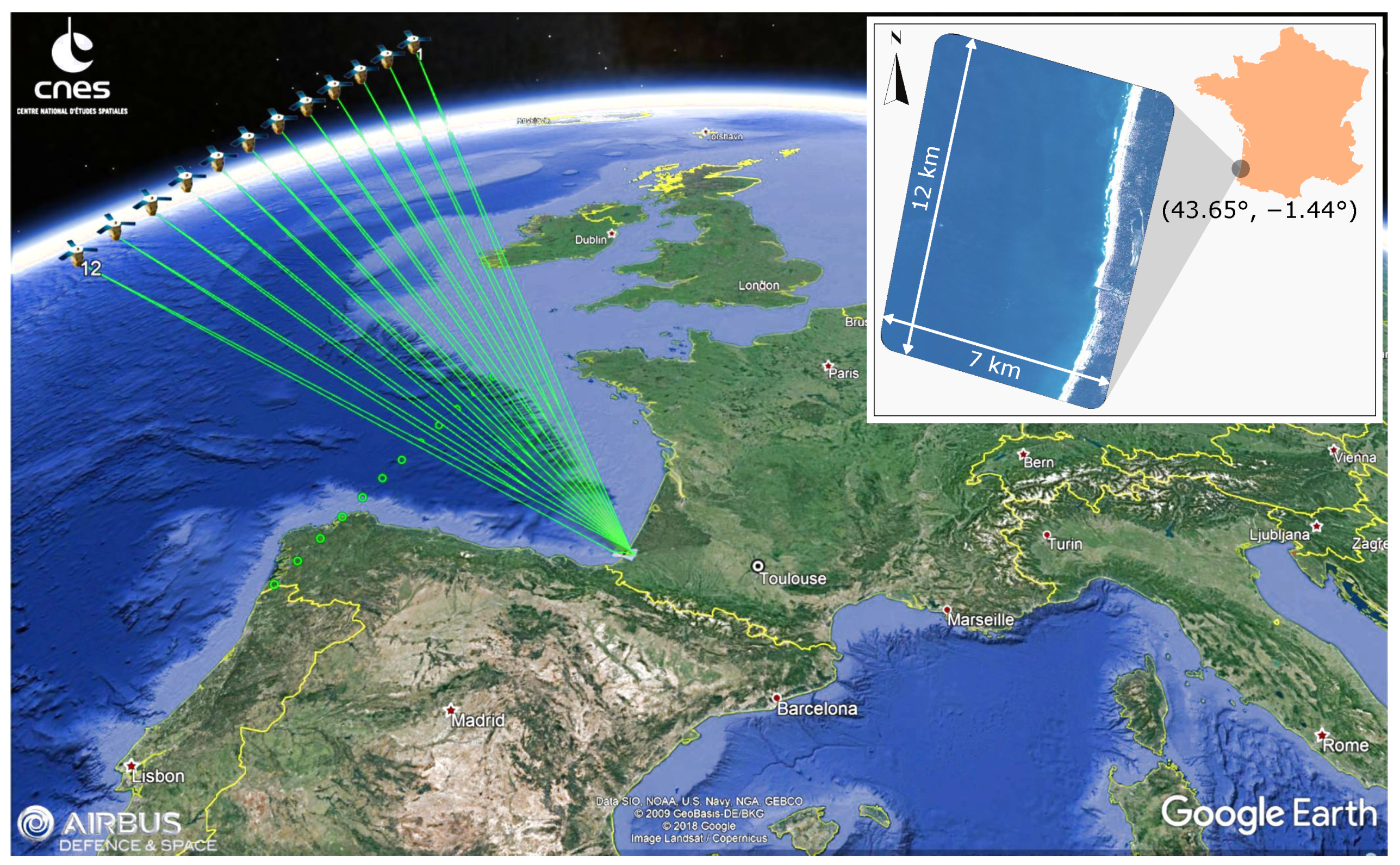
2. Field Site and Data

The data used in this study were acquired during the COMBI Capbreton 2017 field experiment by the Airbus/CNES Pleiades mission [35]. Capbreton, in southwestern France, was chosen as a showcase due to its unique complex bathymetry around a deep underwater canyon [36,37] (Figure 1), providing a large range of depths. In a single pass-over, the Pleiades satellite took 12 consecutive images of the target site at ∼8 s intervals and a resolution of 0.7 m. These images were then orthorectified with homologue ground points using SRTM30 DEM and the SIGMA software of CNES. As such, a superimposable image sequence of an area spanning 12 km alongshore by 7 km cross-shore was established. A bathymetric survey of this region from 2010 [37] was fused to nearshore surveys from the COMBI project to generate a ground truth reference map. On the day of recording, 18 November 2017, at 11h35, hydrodynamic conditions were governed by swell waves arriving from northwesterly directions at 315°, with a significant wave height $H_s=2.0$ m and a peak period of $T_p=11.6$ s.

3. Method

To derive bathymetry from temporally sparse satellite imagery with a standard frequency-based depth inversion method, a two-step approach was explored. First, the sparse image sequence (1/8 fps) was augmented to continuous video (1 fps) as of Almar et al. [34]. Second, this video was processed using the depth inversion algorithm of Gawehn et al. [13]. Core elements of both methods are summarized in Section 3.1 and Section 3.2 respectively.

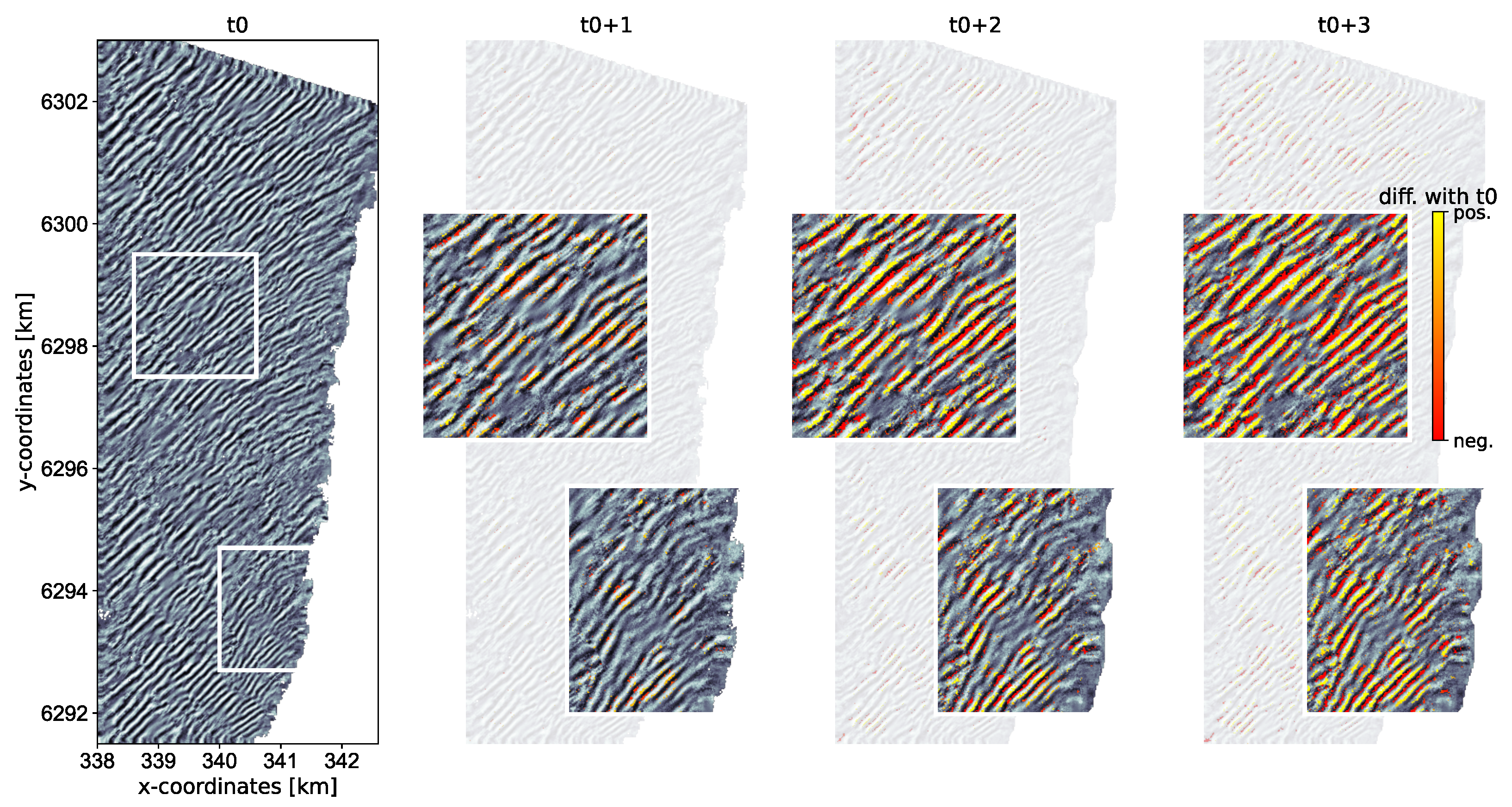
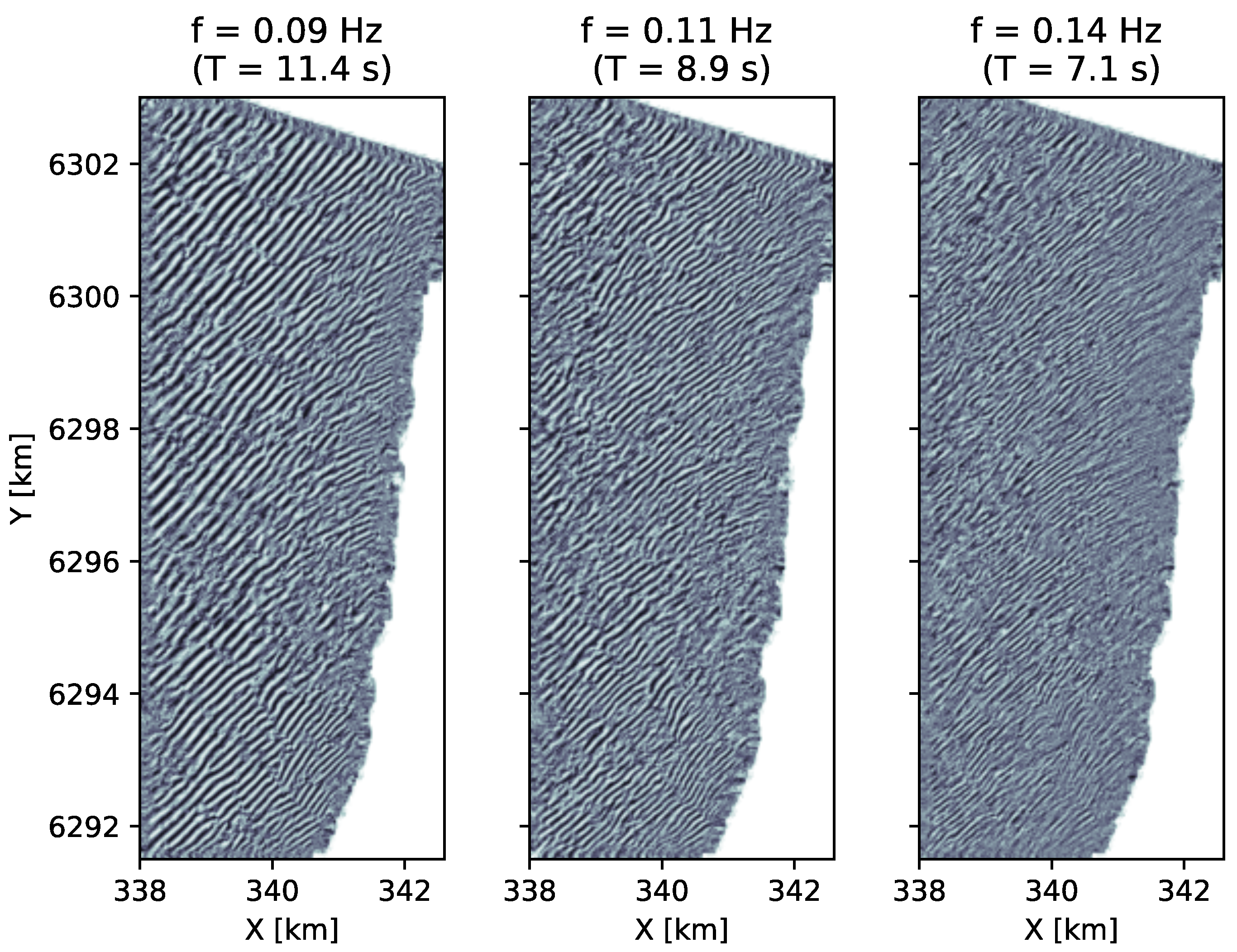
3.1. Temporal Image Augmentation

For augmenting sparse temporal information with dense spatial information a physical principle related to local wave celerity was used. If travel speed and direction of waves at some point in an image are known, it can be hindcasted where these waves were in the recent past and where they will be in the near future. Hence, by looking at different distances from a certain point, stochastic evidence can be found for the time series in that point. This process is repeated for all pixels in an image. The ensemble of time series from all these pixels shows the reconstructed video of the moving wave field. The augmentation process represents a stochastic spatiotemporal interpolation, which increases the frequency resolution and extends the Nyquist frequency (as shorter period oscillations can be reconstructed, see [34] Figure 4). It adds frames and counteracts aliasing [16] and thereby specifically aims to prepare for frequency-based analysis with conventional depth inversion algorithms (typically requiring at least ∼64 frames [13,15]).

Since the video reconstruction process builds on knowledge of local wave celerity, the accuracy of the celerity determines the quality of the resulting video. Due to the limited temporal images in the raw satellite imagery, the local wave celerity vectors need to be approximated. The wave celerity vectors are determined through spatiotemporal cross-correlation in combination with a Radon transform as of [16,34]. Note that there exists an ambiguity in the celerity vector orientation of 180° (i.e., waves could just as well travel in an opposite direction). Here, the wave direction was postulated to be towards the coast, by only considering the signal within 0–90° (Eastward) in Radon polar space. The method could, however, pick the correct direction by ruling out the unrealistic travel speed of the opposite direction. For this study, images were reconstructed from multiple pass-band filtered images. This was performed in the spatial domain using the deep water linear wave dispersion for periods ranging from 5–20 s.

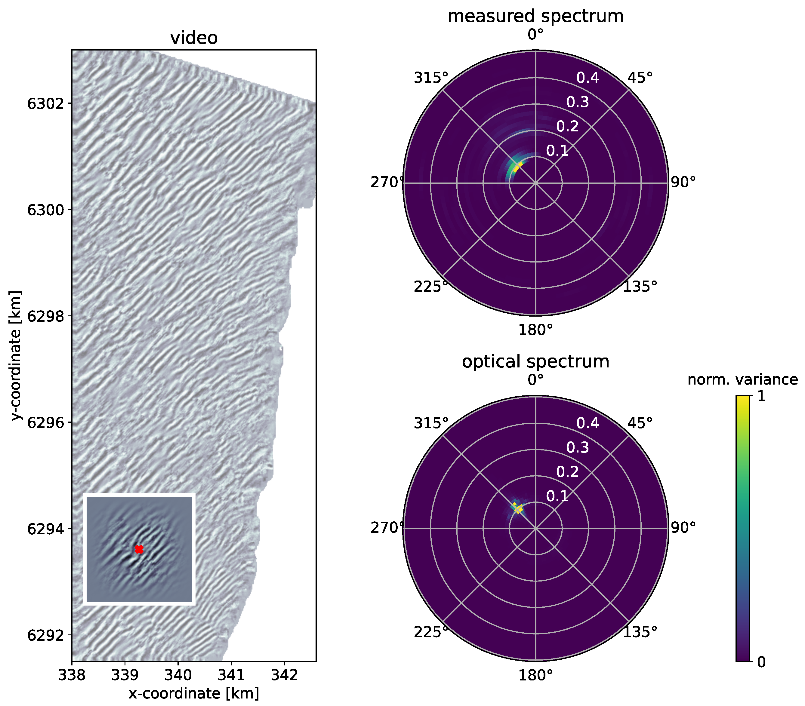
3.2. Frequency-Based Depth Estimation

The algorithm that was used to estimate depths from the augmented satellite video was recently developed and chosen because of its generally accurate performance and open accessibility. The algorithm was built to automatically adapt to given video data and to be computationally fast [13]. Its performance relies on a skill-bed, which largely shows errors in the submeter range. To date, the algorithm has not been tested on augmented spaceborne video, which is a novelty in this study.

One of the key principles of the depth inversion algorithm is to reduce data complexity. For this purpose, a dimensionality reduction technique is employed. It comes in the form of the Dynamic Mode Decomposition (DMD), which allows us to automatically extract main wave features and corresponding frequencies from given video of a moving wave field. The wave features are captured by the dynamic modes, which closely relate to so-called “global one-component phase images” (GOCPI) [13]. Similar to other depth inversion algorithms [15,24,30], such phase images are used to estimate local wavelengths and are therefore a key part of the depth inversion procedure. The GOCPI and their corresponding frequencies can be extracted from relatively short image sequences (64 frames in [13]), which is attractive for the current application. Knowing the dominant frequencies at an early stage, proper sampling schemes can be determined to find local wavenumbers in the GOCPI. Combining frequencies and wavenumbers, local wave spectra are formed, which expect to reflect natural wave dispersion properties. Under this assumption, the Doppler-shifted linear dispersion relationship aids as a theoretical model that can be fitted to the observed spectral data to estimate local depths.

The algorithm automatically determines the grid resolution for efficient processing. For large-scale bathymetry estimation as discussed in Section 4, this grid resolution is 100 m. In the discussion Section 5.2, a local, smaller scale depth inversion analysis is performed with 22 m grid resolution.

Although the algorithm aims to avoid manual adjustment of settings, the reconstructed satellite video presented a challenging case as the displayed wave hydrodynamics represented an approximation to the real wave field. In addition, a large portion (67%) of the observed area is relatively deep >15 m, which means that depth-induced changes in wave characteristics are limited and therefore harder to detect. We found that slight changes to parameter settings offer improvement for the deeper regions. Changes compared to Gawehn et al. [13] are listed in Appendix A 

Table A1. Default parameter values of the depth inversion algorithm.

Parameter	Value
overlap	56 s (in [13]: 16 s)
time analytic extension	False (in [13]: True)
maximum subdomain size per frequency	$2.5\times L_{off}\left({\omega }^{\uparrow }\right)$ (in [13]: $2.0\times L_{off}\left({\omega }^{\uparrow }\right)$)
${\Gamma }_{max}$	$1.2$ (in [13]: $1.0$)
$\alpha$	0.0075 (conform 1 fps video)

. Most importantly, some leeway is given for maximum wave lengths. In the deeper regions, several wave components are close to their theoretical offshore wave length limit ($L/L_{off}={\Gamma }_{max}\approx 1$). To capture this from noisy spectra, detected wavelengths are allowed to marginally exceed this theoretical limit (${\Gamma }_{max}=1.2$, Appendix A Table A1). It gives leeway for the spectral data cloud to scatter (uniformly) around the deep water dispersion limit and thereby allows for an unbiased fit of the dispersion shell to the data. Further improvement for the deeper regions is gained by slightly increasing the grid cell size. It causes depth estimates to be a little less localized, but the larger sampling area increases the accuracy of the wavelength estimates offshore.

4. Results

The reconstructed video and the following depth inversion are respectively presented in Section 4.1 and Section 4.2.

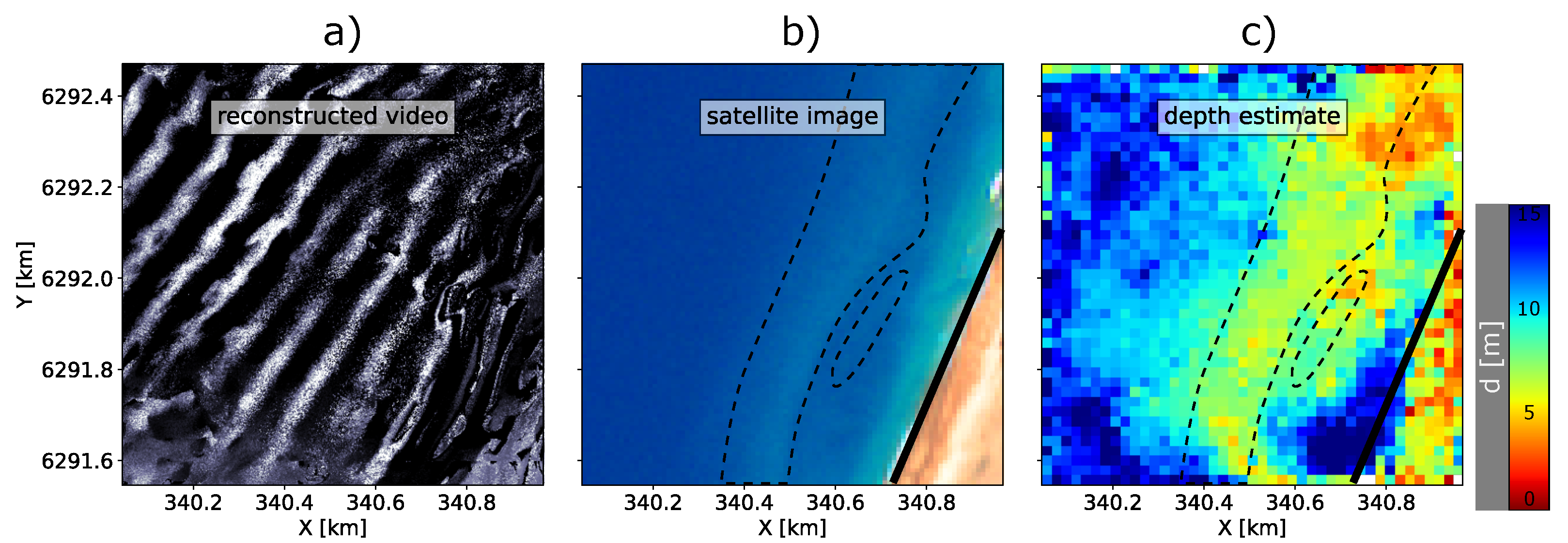
4.1. Results from the Augmentation

Augmentation of the 12 Pleiades images to 1 fps video yields 93 frames. The total length of the video thereby spans just over 1.5 min. Wave patterns are spatially homogenous and show offshore waves to refract and wavelengths to get smaller as they approach the coastline (see Figure 2, $\mathrm{t}0$). Wave motion is continuous and appears realistic for large parts of the domain (Figure 2, upper boxes). Some small patches exist where the reconstruction quality is lower based on visual assessment (Figure 2, lower boxes). Especially near the image or natural boundaries, the augmentation proves more difficult. Fewer spatial points can be used for time-series reconstruction at those locations. In addition, depth estimation near the coastline is particularly challenging as the time-series reconstruction becomes less accurate due to complex wave patterns and wave breaking.

To assess whether wave motion in the reconstructed video reflects reality, the optical spectrum of the video was subsampled around and compared against the measured spectrum from a local wave-buoy (Figure 3) (see also [38]). The optical spectrum displayed the highest variance density at ∼315° and at frequencies of 0.09–0.13 Hz which was consistent with the buoy measurements. Angular wave spreading was less pronounced than in the buoy data. This difference may be ascribed to a combination of artefacts from both the buoy data as well as the video reconstruction procedure. Pitch and roll buoys have the tendency to produce broader spectra than reality, especially in case of narrow-banded spectra [39] (Figure 3, top right). The video reconstruction procedure has the opposite tendency, as it determines wave directions unidirectionally from the Radon-transform [34] (Figure 3, bottom right). Considering these spectral artefacts, the variance density spectra from the in situ buoy and the reconstructed video suggest that the reconstructed video captured the wave field.

So far, the quality assessment of the reconstructed video reveals that wave motion is continuous (Figure 2) and that local optical spectra compare with measured wave spectra (Figure 3). While the presented spectra provide directional information about dominant wave periods, they do not couple them to wave lengths. Since this coupling is crucial for estimating depths via the dispersion relationship, the spatial structure of the dominant frequency components was checked. This was performed by inspecting the global one-component phase images (GOCPI) per frequency component, gained from the depth inversion algorithm [13] used here (Figure 4). For the reconstructed video, the GOCPI depict coherent, long-crested wave patterns in line with a swell wave climate. Moreover, spatial scales and time scales match, as wave lengths decrease for shorter period waves (Figure 4, left to right). Overall, the quality assessment of the reconstructed video thereby suggests a solid basis for depth inversion analysis.

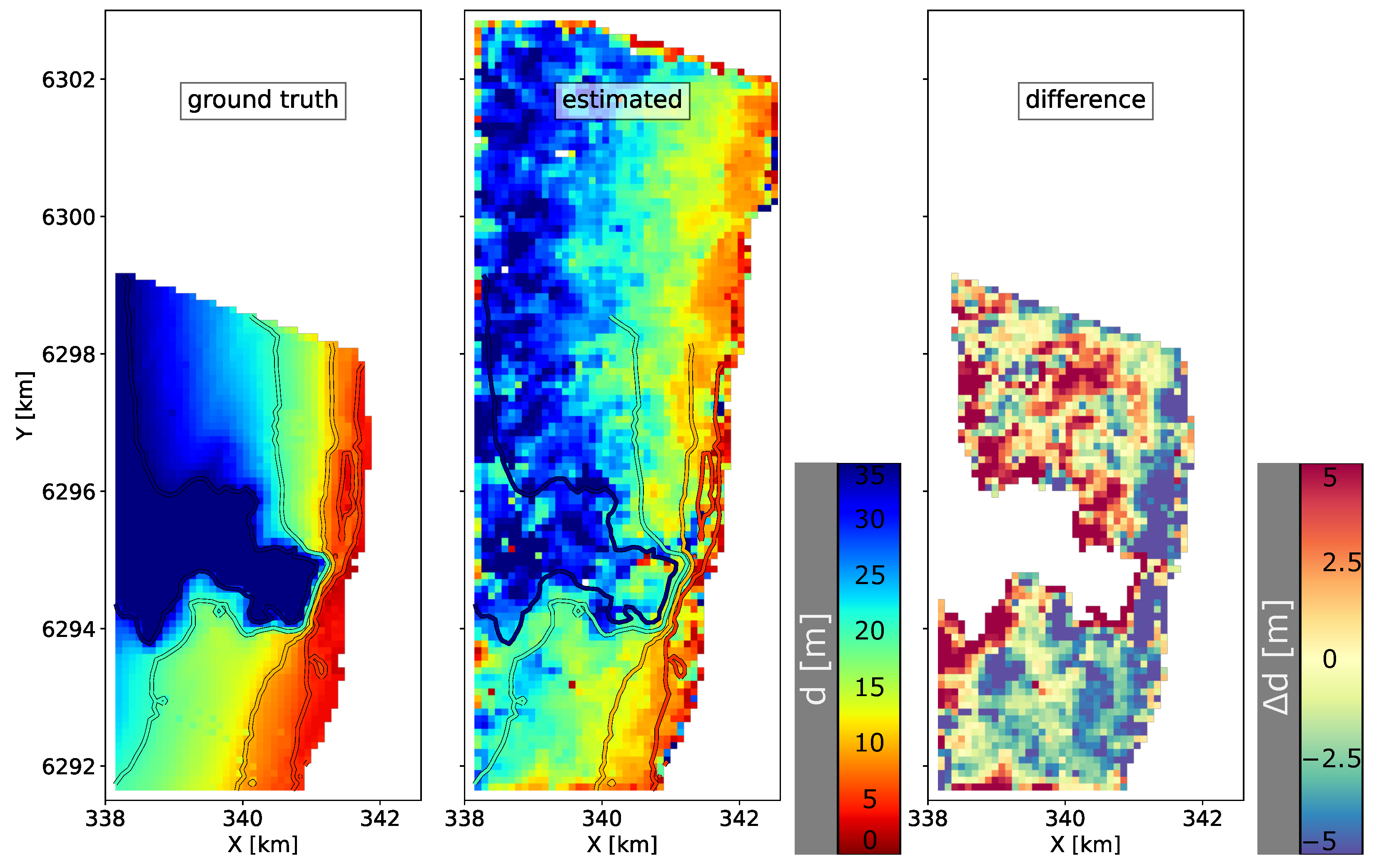
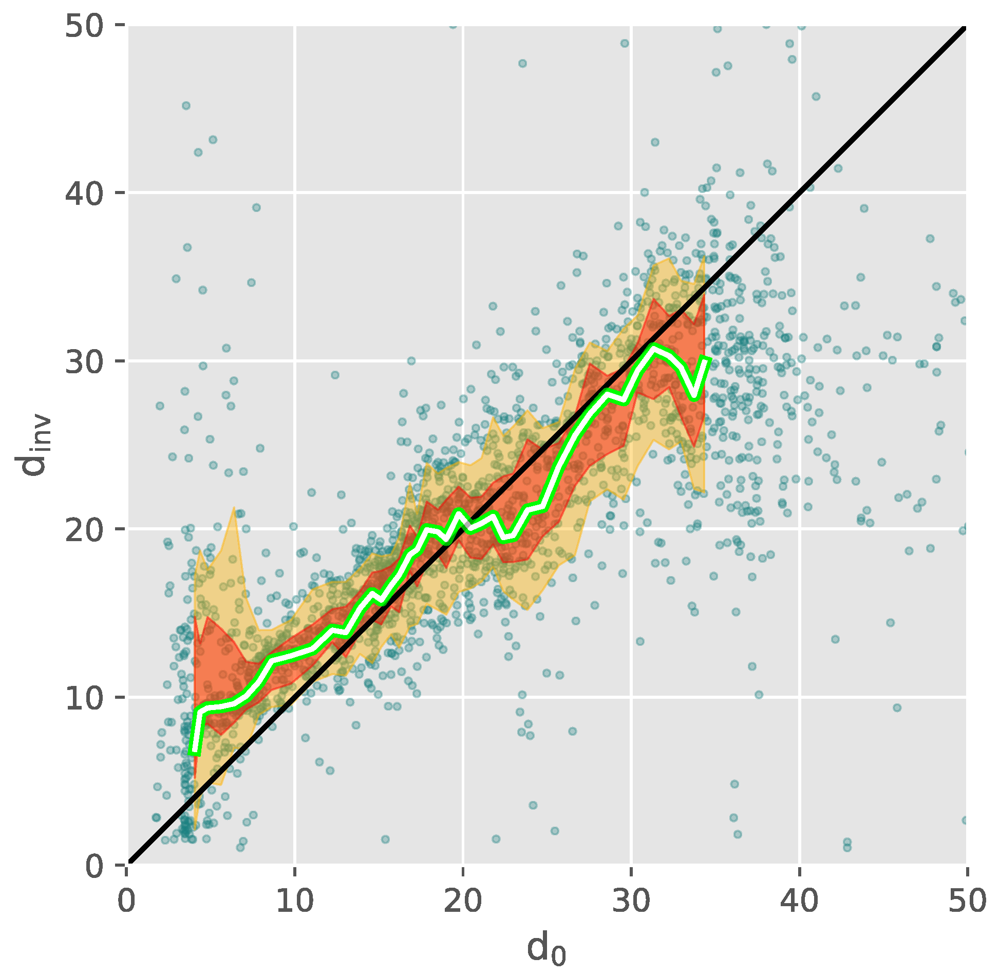
4.2. Results from Depth Inversion

Depth results underscore the potential of combining video reconstruction with a standard frequency-based depth inversion technique (Figure 5). The estimated depth map correctly represents the overall shoreface from the shoreline down to the deeper offshore at ∼35 m (Figure 5 centre). The location of the underwater canyon is also captured, albeit not its depth, which extends to ∼200 m (Figure 5 left). At such depths, waves are no longer significantly affected by the bathymetry, and therefore the depth comparison should be considered as a weak proxy. Errors in the depth estimates are largely <±5 m (Figure 5 right). Mostly around the edge of the canyon and near the shoreline, errors are larger. The edge of the canyon features sharp depth gradients, which are difficult to capture because wave patterns are reconstructed [34] and analysed [13] using spatial sampling areas, and wave attenuation is not instant. Similar situations occur in areas close to the coastline. Employing less usable spatial samples to locally reconstruct time series in combination with wave breaking causes inconsistencies in wave propagation (see also Figure 2, lower white box), eventually leading to noisy depth estimates. Yet, for the most part, the depth estimates approximate ground truth (Figure 5 right, light areas).

The distribution of errors over depth was further studied through a direct comparison between estimated depths and ground truth (Figure 6). The median estimate over depth closely follows the ground truth (cf. Figure 6, green and black lines) and thereby highlights a small overall depth bias of −0.9 m. Depth estimates are scattered, which is quantified by the interquartile range (IQR) (Figure 6, red shaded band), which averages to IQR $=5.1$ m. As indicated by the spatial differences in the depth error (Figure 5 right), this scatter in the depth estimates is larger in shallow parts where $d<\sim 7$ m and deeper parts where $d>\sim 23$ m. For the depth range in between, the scatter appears to be smaller. In the near-coastal region with depths up to 15 m, the IQR averages 3.6 m, which is small considering the fact that estimates were originally extracted from just a few temporally sparse satellite snapshots.

Note that some error in the statistics can probably be attributed to morphological changes that occurred between the time of ground truth measurements, mostly dating from 2010, and the time of depth estimates in 2017. Possible depth errors due to surface current effects are expected to be limited as both measured and estimated surface currents were weak. An ADCP recorded current magnitudes of 2–21 cm s⁻¹ (10th–90th percentile), which is representative of typical tidal current magnitudes at Capbreton [40]. Currents impose a Doppler-shift, which the depth inversion algorithm seeks to take into account. Here, this is challenging due to the unidirectionality of waves, but the algorithm estimated near-surface current magnitudes to be mostly <26 cm s⁻¹ (90% of the estimated area), which is in line with ADCP measurements and also suggests a limited effect on inverted depths.

5. Discussion

The upcoming Section 5.1 discusses the possible use of the large-scale bathymetry estimates for predicting and mapping coastal hydrodynamics. Coastal morphodynamics typically occur in the active coastal zone and may produce nearshore features such as sandbars. Section 5.2 explores whether such sandbars can be captured.

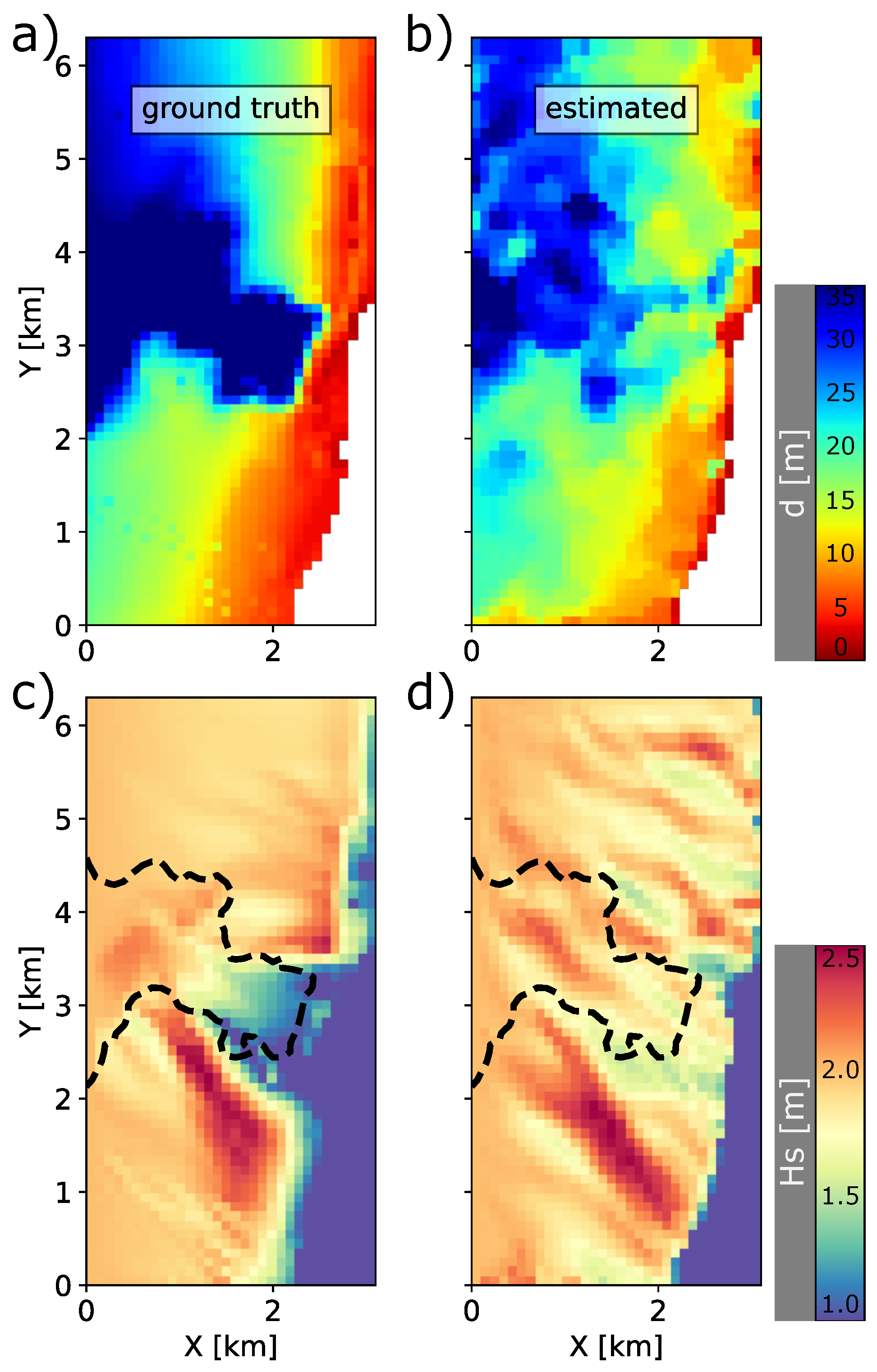
5.1. Using Satellite-Derived Depths for Coastal Wave Height Predictions

While the estimated bathymetry map of Capbreton approximates reality, the question arises whether it can be used for practical applications, such as for wave height predictions over the coastal shoreface along the coast. Such predictions are typically made with numerical models in which the local detailed bathymetry is a required boundary condition to propagate wave energy. It is worthwhile exploring whether the large-scale, satellite-derived bathymetry could substitute for this purpose, as local ground truth data may not always be available.

A straightforward stationary wave model was used to compute wave refraction and the spatial distribution of wave heights at Capbreton [41]. It repeatedly solves the wave action balance and includes dissipation formulations for wave breaking and bottom friction [42,43]. The model was applied to the estimated bathymetry (Figure 7b) as well as the ground truth bathymetry (Figure 7a), and the resulting wave height distributions (Figure 7c,d) were then qualitatively compared. To mitigate the influence of salt-and-pepper noise, the estimated bathymetry data were first filtered with a small $3\times 3$ median filter. The numerical model was forced, using the hydrodynamic conditions observed by the offshore wave buoy during overpass of the satellite ($H_s=2$ m, $T_p=11$ s, wave direction = 315°) (see also Figure 3).

The computed wave heights at Capbreton displayed a characteristic pattern of increased wave heights to the south and north of the canyon and lower wave heights at the canyon head (Figure 7c,d). This is consistent with earlier observations for typical winter month conditions at this site [44]. Wave height predictions using the estimated bathymetry (Figure 7d) were noisier than for the ground truth bathymetry (Figure 7c). Smaller wave heights at the head of the canyon were less pronounced (Figure 7d) because the canyon depth was underestimated there (Figure 7b). However, the increased wave heights to the north and especially the south of the canyon were captured. Submarine canyons are known to refract waves in complex patterns, leading to a variable distribution of wave heights along the coast [45]. Local focusing of wave energy typically causes hotspots of increased wave height, which may be associated to popular locations for wave surfing [44,46]. In this case, the southern band of increased wave heights leads up to a beach called La Piste, a renowned surfing spot (Figure 8). Being able to recognize such wave energy hotspots from satellite-derived bathymetries is also valuable for safety purposes, as hotspots are a determining factor in coastal hazard assessments [1]. At La Piste, wave focusing also contributes to observed shoreline and dune retreat (Figure 8).

5.2. Satellite-Derived Sandbars

The Capbreton bathymetry is complex, featuring a large underwater canyon, but also fine sandbar structures along the adjacent coastline. Sandbars are an important element for understanding coastal systems [47], and it would therefore be valuable to capture them.

Sandbars are relatively small morphological features, and therefore, they require a more detailed depth inversion analysis. Zooming in on the location of a sandbar at Capbreton, a refined local wave-field video was reconstructed with a framerate of 2 fps (Figure 9a). As these sandbars are located in the nearshore region with characteristic depths of 0–15 m (Figure 9b), the depth inversion analysis (Figure 9c) was performed using the standard algorithm settings of Gawehn et al. [13].

The estimated sandbar morphology (Figure 9c) was qualitatively compared to the sandbar position visible through optical imagery (Figure 9b). Ground truth bathymetry data were too coarse and outdated in this area. The comparison showed that the local depth inversion analysis distinctly captured the sandbar morphology. Approaching the sandbar from offshore, the water depth decreased up to the position of the sandbar at an estimated depth of ∼5 m, which is in line with expectations for this site [37]. This was then followed by a trough shoreward of the sandbar and eventually the coastline. The analysis demonstrates that the proposed depth inversion methodology can expose small-scale features from optical satellite imagery and may thereby add morphological detail in regions with absent or coarse knowledge of the present bathymetry. Sandbar estimates could potentially be improved using wave breaking and dissipation as an additional proxy for depth [48,49] or be combined with depth estimates from satellite SAR imagery on cloudy days [50,51].

6. Conclusions

This study explored the estimation of coastal bathymetry from satellite imagery with a frequency-based depth inversion method. Wave-based depth inversion methods in the frequency domain share a large user community and are widely applied to derive bathymetry from video of camera stations, UAVs and Xband-radars. It would therefore be appealing if these standard methods could also be used on satellite imagery. However, as is, the temporal resolution of satellite imagery remains sparse. To enable frequency-based depth inversion to work, satellite imagery was temporally augmented in this study, which was achieved using pre-existing techniques. As such, depth inversion becomes a two-step process, with the first step being the augmentation of sparse satellite imagery to video, and the second step being the analysis of this video with a frequency-based depth inversion method. As a proof of concept, Pleiades images of the study site Capbreton in France were temporally augmented from originally 1/8 fps to 1 fps video lasting just over 1.5 min. The resulting augmented video showed smooth propagation of wave crests, and its spectral content accurately represented in situ buoy measurements. The video was subsequently analysed using a frequency-based depth inversion algorithm, which works largely unsupervised and is openly accessible. The resulting depth estimates approximated the ground truth with an overall depth bias of −0.9 m, yet estimates were spatially noisy with an interquartile range of depth errors of 5.1 m. Still, the acquired accuracy was sufficiently high to correctly predict wave heights over the shoreface with a numerical wave model and to find hotspots where wave refraction leads to focussing of wave energy that has potential implications for coastal hazard assessments. Furthermore, detailed depth inversion analysis of the nearshore region demonstrated the potential to capture small-scale morphological features such as sandbars. This study demonstrates that pre-existing techniques can be combined to estimate bathymetry from satellite imagery and that these estimated bathymetries may serve coastal management purposes.

References

1. Van Dongeren, A.; Ciavola, P.; Martinez, G.; Viavattene, C.; Bogaard, T.; Ferreira, O.; Higgins, R.; McCall, R. Introduction to RISC-KIT: Resilience-increasing strategies for coasts. Coast. Eng. 2018, 134, 2–9. [Google Scholar] [CrossRef] [Green Version]
2. Davidson, M.; Aarninkhof, S.; Van Koningsveld, M.; Holman, R. Developing coastal video monitoring systems in support of coastal zone management. J. Coast. Res. 2006, 2004, 49–56. [Google Scholar]
3. De Schipper, M.A.; Ludka, B.C.; Raubenheimer, B.; Luijendijk, A.P.; Schlacher, T.A. Beach nourishment has complex implications for the future of sandy shores. Nat. Rev. Earth Environ. 2021, 2, 70–84. [Google Scholar] [CrossRef]
4. Almar, R.; Ranasinghe, R.; Bergsma, E.W.; Diaz, H.; Melet, A.; Papa, F.; Vousdoukas, M.; Athanasiou, P.; Dada, O.; Almeida, L.P.; et al. A global analysis of extreme coastal water levels with implications for potential coastal overtopping. Nat. Commun. 2021, 12, 1–9. [Google Scholar] [CrossRef]
5. Vitousek, S.; Barnard, P.L.; Fletcher, C.H.; Frazer, N.; Erikson, L.; Storlazzi, C.D. Doubling of coastal flooding frequency within decades due to sea-level rise. Sci. Rep. 2017, 7, 1–9. [Google Scholar] [CrossRef]
6. Almar, R.; Bergsma, E.W.; Thoumyre, G.; Baba, M.W.; Cesbron, G.; Daly, C.; Garlan, T.; Lifermann, A. Global satellite-based coastal bathymetry from waves. Remote Sens. 2021, 13, 4628. [Google Scholar] [CrossRef]
7. Bergsma, E.W.; Almar, R. Coastal coverage of ESA’ Sentinel 2 mission. Adv. Space Res. 2020, 65, 2636–2644. [Google Scholar] [CrossRef]
8. Li, J.; Roy, D.P. A global analysis of Sentinel-2a, Sentinel-2b and Landsat-8 data revisit intervals and implications for terrestrial monitoring. Remote Sens. 2017, 9, 902. [Google Scholar] [CrossRef] [Green Version]
9. Lyzenga, D.R. Remote sensing of bottom reflectance and water attenuation parameters in shallow water using aircraft and landsat data. Int. J. Remote Sens. 1981, 2, 71–82. [Google Scholar] [CrossRef]
10. Stumpf, R.P.; Holderied, K.; Sinclair, M. Determination of water depth with high-resolution satellite imagery over variable bottom types. Limnol. Oceanogr. 2003, 48, 547–556. [Google Scholar] [CrossRef]
11. Abileah, R. Mapping shallow water depth from satellite. Am. Soc. Photogramm. Remote Sens. 2006, 1, 1–7. [Google Scholar]
12. Stockdon, H.F.; Holman, R.A. Estimation of wave phase speed and nearshore bathymetry from video imagery. J. Geophys. Res. Ocean. 2000, 105, 22015–22033. [Google Scholar] [CrossRef]
13. Gawehn, M.; de Vries, S.; Aarninkhof, S. A Self-Adaptive Method for Mapping Coastal Bathymetry On-The-Fly from Wave Field Video. Remote Sens. 2021, 13, 4742. [Google Scholar] [CrossRef]
14. Holman, R.A.; Brodie, K.L.; Spore, N.J. Surf Zone Characterization Using a Small Quadcopter: Technical Issues and Procedures. IEEE Trans. Geosci. Remote Sens. 2017, 55, 2017–2027. [Google Scholar] [CrossRef]
15. Simarro, G.; Calvete, D.; Luque, P.; Orfila, A.; Ribas, F. UBathy: A new approach for bathymetric inversion from video imagery. Remote Sens. 2019, 11, 2722. [Google Scholar] [CrossRef] [Green Version]
16. Almar, R.; Bergsma, E.W.; Gawehn, M.A.; Aarninkhof, S.G.; Benshila, R. High-frequency Temporal Wave-pattern Reconstruction from a Few Satellite Images: A New Method towards Estimating Regional Bathymetry. J. Coast. Res. 2020, 95, 996–1000. [Google Scholar] [CrossRef]
17. Bergsma, E.W.; Almar, R.; Maisongrande, P. Radon-augmented Sentinel-2 satellite imagery to derive wave-patterns and regional bathymetry. Remote Sens. 2019, 11, 1918. [Google Scholar] [CrossRef] [Green Version]
18. Gabor, D. A Theory of Communication. J. Inst. Electr. Eng.-Part III Radio Commun. Eng. 1946, 93, 429–441. [Google Scholar] [CrossRef]
19. Almeida, L.P.; Almar, R.; Bergsma, E.W.; Berthier, E.; Baptista, P.; Garel, E.; Dada, O.A.; Alves, B. Deriving high spatial-resolution coastal topography from sub-meter satellite stereo imagery. Remote Sens. 2019, 11, 590. [Google Scholar] [CrossRef] [Green Version]
20. Abileah, R. Mapping near shore bathymetry using wave kinematics in a time series of WorldView-2 satellite images. Int. Geosci. Remote Sens. Symp. (IGARSS) 2013, 2, 2274–2277. [Google Scholar] [CrossRef]
21. Almar, R.; Bergsma, E.W.; Maisongrande, P.; de Almeida, L.P.M. Wave-derived coastal bathymetry from satellite video imagery: A showcase with Pleiades persistent mode. Remote Sens. Environ. 2019, 231, 111263. [Google Scholar] [CrossRef]
22. De Michele, M.; Raucoules, D.; Idier, D.; Smai, F.; Foumelis, M. Shallow bathymetry from multiple sentinel 2 images via the joint estimation of wave celerity and wavelength. Remote Sens. 2021, 13, 2149. [Google Scholar] [CrossRef]
23. Abessolo Ondoa, G.; Almar, R.; Castelle, B.; Testut, L.; Léger, F.; Sohou, Z.; Bonou, F.; Bergsma, E.W.; Meyssignac, B.; Larson, M. Sea level at the coast from video-sensed waves: Comparison to tidal gauges and satellite altimetry. J. Atmos. Ocean. Technol. 2019, 36, 1591–1603. [Google Scholar] [CrossRef]
24. Holman, R.; Plant, N.; Holland, T. CBathy: A robust algorithm for estimating nearshore bathymetry. J. Geophys. Res. Ocean. 2013, 118, 2595–2609. [Google Scholar] [CrossRef]
25. Bergsma, E.W.; Almar, R.; Melo de Almeida, L.P.; Sall, M. On the operational use of UAVs for video-derived bathymetry. Coast. Eng. 2019, 152, 103527. [Google Scholar] [CrossRef]
26. Holman, R.A.; Holland, K.T.; Lalejini, D.M.; Spansel, S.D. Surf zone characterization from Unmanned Aerial Vehicle imagery. Ocean Dyn. 2011, 61, 1927–1935. [Google Scholar] [CrossRef]
27. Bell, P. Shallow water bathymetry derived from an analysis of X-band marine radar images of waves. Coast. Eng. 1999, 37, 513–527. [Google Scholar] [CrossRef]
28. Gawehn, M.; van Dongeren, A.; de Vries, S.; Swinkels, C.; Hoekstra, R.; Aarninkhof, S.; Friedman, J. The application of a radar-based depth inversion method to monitor nearshore nourishments on an open sandy coast and an ebb-tidal delta. Coast. Eng. 2020, 159, 103716. [Google Scholar] [CrossRef]
29. Honegger, D.A.; Haller, M.C.; Holman, R.A. High-resolution bathymetry estimates via X-band marine radar: 1. beaches. Coast. Eng. 2019, 149, 39–48. [Google Scholar] [CrossRef]
30. Senet, C.M.; Seemann, J.; Flampouris, S.; Ziemer, F. Determination of bathymetric and current maps by the method DiSC based on the analysis of nautical X-band radar image sequences of the sea surface (November 2007). IEEE Trans. Geosci. Remote Sens. 2008, 46, 2267–2279. [Google Scholar] [CrossRef]
31. Bell, P. Mapping Shallow Water Coastal Areas Using a Standard Marine X-Band Radar. In Proceedings of the Hydro8, Liverpool, UK, 4–6 November 2008; International Federation of Hydrographic Societies: Lemmer, The Netherlands, 2008; pp. 1–9. [Google Scholar]
32. Holman, R.; Bergsma, E.W. Updates to and performance of the cbathy algorithm for estimating nearshore bathymetry from remote sensing imagery. Remote Sens. 2021, 13, 3996. [Google Scholar] [CrossRef]
33. Palmsten, M.L.; Brodie, K.L. The Coastal Imaging Research Network (CIRN). Remote Sens. 2022, 14, 453. [Google Scholar] [CrossRef]
34. Almar, R.; Bergsma, E.W.; Maisongrande, P.; Giros, A.; Almeida, L.P. On the application of a two-dimension spatio-temporal cross-correlation method to inverse coastal bathymetry from waves using a satellite-based video sequence. In Proceedings of the 2019 IEEE International Geoscience and Remote Sensing Symposium (IGARSS), Yokohama, Japan, 28 July–2 August 2019; pp. 8205–8208. [Google Scholar] [CrossRef]
35. Coeurdevey, L.; Gabriel-Robez, C. Pléiades Imagery—User Guide; Technical Report; Astrium GEO-Information Services: Toulouse, France, 2012. [Google Scholar]
36. Jouanneau, J.M.; Latouche, C. Continental fluxes to the Bay of Biscay: Processes and behaviour. Ocean Shorel. Manag. 1989, 12, 477–485. [Google Scholar] [CrossRef]
37. Mazières, A.; Gillet, H.; Castelle, B.; Mulder, T.; Guyot, C.; Garlan, T.; Mallet, C. High-resolution morphobathymetric analysis and evolution of Capbreton submarine canyon head (Southeast Bay of Biscay-French Atlantic Coast) over the last decade using descriptive and numerical modeling. Mar. Geol. 2014, 351, 1–12. [Google Scholar] [CrossRef] [Green Version]
38. Almar, R.; Bergsma, E.W.J.; Catalan, P.A.; Cienfuegos, R.; Suarez, L.; Lucero, F.; Nicolae Lerma, A.; Desmazes, F.; Perugini, E.; Palmsten, M.L.; et al. Sea State from Single Optical Images: A Methodology to Derive Wind-Generated Ocean Waves from Cameras, Drones and Satellites. Remote Sens. 2021, 13, 679. [Google Scholar] [CrossRef]
39. Kuik, A.J.; van Vledder, G.P.; Holthuijsen, L.H. A Method for the Routine Analysis of Pitch-and-Roll Buoy Wave Data. J. Phys. Oceanogr. 1988, 18, 1020–1034. [Google Scholar] [CrossRef]
40. Campbell, R.; Martinez, A.; Letetrel, C.; Rio, A. Methodology for estimating the French tidal current energy resource. Int. J. Mar. Energy 2017, 19, 256–271. [Google Scholar] [CrossRef]
41. Booij, N.; Ris, R.C.; Holthuijsen, L.H. A third-generation wave model for coastal regions 1. Model description and validation. J. Geophys. Res. Ocean. 1999, 104, 7649–7666. [Google Scholar] [CrossRef] [Green Version]
42. Baldock, T.E.; Holmes, P.; Bunker, S.; Van Weert, P. Cross-shore hydrodynamics within an unsaturated surf zone. Coast. Eng. 1998, 34, 173–196. [Google Scholar] [CrossRef]
43. Jonsson, I.G. Wave Boundary Layers and Friction Factors. In Coastal Engineering 1966; American Society of Civil Engineers: New York, NY, USA, 1967; pp. 127–148. [Google Scholar] [CrossRef]
44. Lastiri, X.; Abadie, S.; Maron, P.; Delpey, M.; Liria, P.; Mader, J.; Roeber, V. Wave energy assessment in the south aquitaine nearshore zone from a 44-year hindcast. J. Mar. Sci. Eng. 2020, 8, 199. [Google Scholar] [CrossRef] [Green Version]
45. Manian, D.; Kaihatu, J.M.; Zechman, E.M. Using genetic algorithms to optimize bathymetric sampling for predictive model input. J. Atmos. Ocean. Technol. 2012, 29, 464–477. [Google Scholar] [CrossRef]
46. Kaihatu, J.M.; Edwards, K.L.; O’Reilly, W.C. Model predictions of nearshore processes near complex bathymetry. Ocean. Conf. Rec. (IEEE) 2002, 2, 685–691. [Google Scholar] [CrossRef]
47. Bosboom, J.; Stive, M.J.F. Coastal Dynamics; TU Delft Open: Delft, The Netherlands, 2021; p. 595. [Google Scholar] [CrossRef]
48. Aarninkhof, S.G.J.; Ruessink, B.G.; Roelvink, J.A. Nearshore subtidal bathymetry from time-exposure video images. J. Geophys. Res. Ocean. 2005, 110, 1–13. [Google Scholar] [CrossRef]
49. Van Dongeren, A.; Plant, N.; Cohen, A.; Roelvink, D.; Haller, M.C.; Catalán, P. Beach Wizard: Nearshore bathymetry estimation through assimilation of model computations and remote observations. Coast. Eng. 2008, 55, 1016–1027. [Google Scholar] [CrossRef]
50. Jawak, S.D.; Vadlamani, S.S.; Luis, A.J. A Synoptic Review on Deriving Bathymetry Information Using Remote Sensing Technologies: Models, Methods and Comparisons. Adv. Remote Sens. 2015, 4, 147–162. [Google Scholar] [CrossRef] [Green Version]
51. Huang, W.G.; Fu, B.; Zhou, C.B.; Yang, J.S.; Shi, A.Q.; Li, D.L. Shallow water bathymetric surveys by spaceborne synthetic aperture radar. Int. Geosci. Remote. Sens. Symp. (IGARSS) 2001, 6, 2810–2812. [Google Scholar] [CrossRef]
Figure 1. Pleiades satellite collecting 12 images of the field-site Capbreton, France. The observed area and its location (Lat°, Lon°) are depicted in the top right.
Remotesensing 14 01847 g001
Figure 2. First four frames of the reconstructed video at times t 0 = 0 s to t 0 + 3 = 3 s. Wave movement is highlighted by zooming in on two example regions (white boxes), and looking at the difference with respect to t 0 (color scale). Yellow, positive differences point out rising water levels due to incoming wave fronts. Red, negative differences point out the associated falling water levels at the back of the wave. For clarity, only differences >10% are depicted.
Remotesensing 14 01847 g002
Figure 3. Comparison of an in situ measured (left, red ‘x’) variance density spectrum from a local buoy (top right) against a corresponding optical variance density spectrum from reconstructed satellite video (bottom right) of a representative area ( 2   km   ×   2   km ) around the buoy location (left, white box). Both spectra are normalized to unit magnitude for comparison.
Remotesensing 14 01847 g003
Figure 4. Global one-component phase images (GOCPI) of dominant frequency components f = 0.09 , 0.11 , 0.14 Hz in the reconstructed video. The phase images are naturally retrieved via the Dynamic Mode Decomposition as part of the depth inversion procedure [13]. In total, nine phase images are used for analysis, of which three are presented as example.
Remotesensing 14 01847 g004
Figure 5. Comparison of depths, d, from ground truth (left) against depths estimated from reconstructed satellite video (centre). Ground truth depth contours are superimposed on estimated depths for reference. Depths are indicated from red (shallow) to blue (deep) as of centre colour scale. The difference, Δ d , between estimated depths and ground truth, is presented in the right panel, with red/blue, respectively, denoting under-/overestimation of depth (right colour scale). Parts where d > 35 m are masked and indicate the underwater canyon where waves are unaffected by the bathymetry.
Remotesensing 14 01847 g005
Figure 6. Direct comparison of inverted depths, d i n v against ground truth, d 0 (blue dots). The median is indicated in green and aims to approximate the black 1:1 line. The 25th–75th percentile is shaded red and superimposed on the 10th–90th percentile shaded orange.
Remotesensing 14 01847 g006
Figure 7. Predicted wave height distributions over ground truth bathymetry and estimated bathymetry of Capbreton using a numerical wave model: (a,b) ground-truth depths and estimated depths, respectively, used in the model, where red/blue indicate shallow/deep regions (top colorbar). Salt-and-pepper noise has been removed from (b) using a 3 × 3 median filter; (c,d) significant wave height distribution associated to (a,b), respectively, where red/blue indicate high/low wave heights (bottom colorbar). The 35 m depth contour is superimposed to outline the location of the canyon. Hydrodynamic field conditions with H s = 2 m, T p = 11 s and wave direction = 315° measured by a local buoy (see Figure 3) during satellite overpass are used as boundary forcing.
Remotesensing 14 01847 g007
Figure 8. The beach La Piste at Capbreton, France.
Remotesensing 14 01847 g008
Figure 9. Sandbars from depth inversion of a locally reconstructed video of the nearshore wave field: (a) reconstructed video with framerate of 2 fps; (b) satellite image showing the position of the sandbar; (c) depth estimates based on (a); For reference, dashed black contours outline the position of the sandbar. and the solid black line indicates the position of the coastline.
Remotesensing 14 01847 g009
Publisher’s Note: MDPI stays neutral with regard to jurisdictional claims in published maps and institutional affiliations.