1. Introduction
In deep learning, texture and material analyses play an essential role in object classification, detection, and segmentation tasks. This type of analysis has some application areas, such as computer-aided medical diagnosis, fruit recognition using artificial intelligence, and object detection in aerial navigation with drones to mention a few.
Deep learning in the last decade has positioned itself as a new solution in the areas of robotics, computer vision, and natural language [
1,
2,
3]. In particular, Convolutional Neural Networks (CNNs) are a category of deep learning, as they are adapted to object analysis by learning and extracting complex features [
4,
5]. On the other hand, although CNNs is a universal extractor, in practice, it is not clear whether CNNs can learn to perform spectral analysis—a methodology that can provide a better classification performance of textures and materials [
6]. In this sense, a fusion of methods in order to address this problem is being used, combining spatial and spectral approaches in a unique architecture [
7,
8]. Despite the results obtained by the authors in texture classification, their architecture only merges the features that are lost with the spatial approach. In addition, it is known that regularization methods focus only on the convolutional layer. While the operations of the pooling layers have been left without an update [
9]. In this sense, we can integrate wavelet analysis inside deep learning before merging spatial and spectral approaches; that is, we permit it to become part of the learning process by using the pooling method.
Motivated by the above reasons, in this study, we propose a classification system with a new pooling method called Discrete Wavelet Transform Pooling (DWTP). The pooling approach is based on image decomposition into sub-bands. The method is implemented and developed using Python and Keras API with Tensorflow as Backend. Moreover, the method is validated on three datasets: CIFAR-10, Describable Textures Dataset (DTD), and Flickr Material Database (FMD). Our approach is different from traditional methods because it is not a subsampling methodology by using neighboring regions, but wavelet pooling maintains its function as a reduction layer. Wavelets allow localization in scale (i.e., frequency) and space. In other words, wavelets can be used to analyze local and spatial transients in the data, such as edges or surfaces in an image [
10]. Therefore, we can preserve the most relevant information of textures and materials, which is sometimes lost with traditional methods such as Max-Pooling (MaxP) and Ave-Pooling (AveP).
In a previous study, as support for this work in [
11], we designed a CNN architecture for object detection with a repetitive pattern approach within aerial navigation as a first attempt. We argue that the characteristics at different frequencies, low and high, also affect the performance of the CNN during training. This architecture is characterized by wavelet analysis, applying multiresolution analysis to the original image. A new dataset is obtained when the image is converted to the wavelet domain. Therefore, the information improves learning performance, eliminates overfitting, and achieves higher efficiency in object detection. Based on the results from our previous work, we now present a wavelet pooling approach to improve the learning of the classification model with the following contributions:
We present a CNN architecture with a combination of regularization methods (DropOut, Data Augmentation, and Batch Normalization) to evaluate the performance of each pooling method: MaxP, AveP, and wavelet pooling (DWTP, DWTaP, and DWTdP). The objective is to have a reference of the learning behavior.
We present a complete evaluation of the classification performance of textures and materials in images, in addition to a state-of-the-art benchmark dataset. The idea is to evaluate the adaptability of deep learning with wavelet pooling. Furthermore, we argue that the methodology is ideal for this type of dataset, where it is recurrent to have repetitive patterns.
We show that the method eliminates the overfitting created by pooling methods while reducing features using an approach based on level-based decomposition, and it is more compact than pooling by using neighboring regions. Hence, we offer three configurations: DWTP = approximation and detail information; DWTaP = approximation information; and DWTdP = detail information. The goal is to preserve the most information for each texture and material.
We demonstrate that a correct inference of texture or material can be obtained if we determine the type of pooling to be used during learning. We have conducted several experiments, but now we can choose the best pooling method depending on the dataset. Our experiments indicate that this is also useful for future object detection applications, focusing on physical features such as texture.
In order to present our approach, this paper has been organized as follows:
Section 2 shows related work;
Section 3 introduces the methodology to address the texture and material classification problem.
Section 4 shows the proposed methodology. After that,
Section 5 shows the results with the three data sets, which have been used to test our approach and the experimental part. Finally,
Section 6 discusses the results, and
Section 7 presents the conclusions and future work.
2. Related Work
This section highlights some applications that have used the wavelet pooling layer to improve their performance. A new architecture called WaveCNN was proposed in [
12]. They note that the pooling layer (Max-Pooling) in a conventional CNN does not consider the feature structure of the previous layer. Then, Max-Pooling may lose some features. Therefore, they replace the pooling layer with wavelet decomposition. They succeed in more adequately representing the features for MNIST handwritten digit classification. A novel method that combined classical CNN layers with squeeze-and-excitation modules and the Haar wavelet as a pooling layer was proposed by [
13]. The main objective is the real-time classification of vehicle types. The development of the method improves the classifier’s performance by highlighting essential feature maps and decreasing the network entropy. Moreover, they propose a cross-entropy cost function and the use of DWT instead of Max-Pooling to improve the recognition rate. According to this layer, their model is named Wavelet Deep Neural Network (WDNN). Another alternative is the application of a multilevel analysis [
14]. The method merges multiple wavelets transforms, as they function similarly to filters within convolutional neural networks. They show that some neighborhood methods introduce edge halos, aliasing, and blurring effects in specific datasets. Choosing the correct pooling method is key to obtaining good results. Thus, they explore the use of wavelet bases such as Haar, Coiflet, and Daubechies to perform pooling.
In semantic segmentation tasks, encoder–decoder-type networks have been used [
15]. This type of CNNs usually uses pooling to reduce computational costs and improve invariances relative to certain distortions and expands the receptive field. However, pooling can result in information loss, which disruptive to later operations, such as feature extraction and analysis. Moreover, each image pixel is assigned a specific class in semantic segmentation tasks by dividing it into regions of interest. Therefore, a pooling method based on wavelet operations has been proposed to divide it into regions of interest. In [
16], the authors presented an approach called 3D WaveUNet, based on wavelets and deep learning for 3D neuron segmentation. The encoder-decoder network is integrated with a 3D wavelet to segment the nerve fibers into cubes; the wavelets help the deep networks remove noise from the data and connect the broken fibers. At the end of the method, the segmented nerve fibers into cubes are assembled to generate the entire neuron. In this case, the neuron segmentation method can completely extract the target neuron in noisy neuron images. A U-Net architecture based on wavelet transform pooling is proposed in [
17]. This work aims to segment multiple sclerosis (MS) lesions in magnetic resonance images (MR). One characteristic is that the first stage of the network uses the wavelet transform, and in the second stage, its inverse is used. In both stages, it highlights abrupt changes in the image and better describes the features. An advantage is its multiresolution analysis; thus, its use improves the detection of lesions of different sizes and in segmentation.
In the area of image restoration, a multilevel wavelet CNN (MWCNN) method was proposed to balance the size of the receptive area and computational efficiency [
18]. The main idea is to integrate the wavelet transform within the CNN architecture to reduce feature maps. The MWCNN method is also based on a U-Net architecture and the inverse wavelet transform (IWT) for the reconstruction stage with a high resolution. In [
9], they proposed another alternative called wavelet pooling as a layer inside the CNN architecture. This method decomposes the image into two sub-bands, discarding the first level to reduce the size of the feature map. The approach allows a structured compression of the data, reducing the creation of denoised edges and other defects in the image.
On the other hand, some works have employed deep learning and wavelet analysis in image processing. For example, the method proposed in [
19] converted images from the CIFAR-10 and KDEF database to the wavelet domain, thus obtaining temporal and frequency features. The different representations created are added to multiple CNN architectures. This combination of information in the wavelet domain achieves a higher detection efficiency and a faster execution time than the procedure in the spatial domain.
In the automatic coding of an image, the design of the CNN architecture has a significant weight. In this case, the designed network is a Siamese convolutional neural network that receives fused information from infrared and visible images. The aim is to generate a weight map representing the saliency of each pixel. Fusion is performed by multiscale decomposition of the image using wavelet analysis, and the reconstruction result is more perceptual to the human visual system [
20]. Following the same approach, the work proposed in [
21] presented two methods to highlight the edges of the images in the classification area. The first method decomposes the images and subsequently reconstructs them in a limited manner. The second method that develops the enhanced images introduces local maximum wavelet coefficients. Both methods are applied before entering the CNN architecture.
3. Materials and Methods
3.1. Wavelet Analysis
Wavelets represent functions as simpler, fixed building blocks at different scales and positions [
19]. The one-dimensional wavelet transform can be easily extended to a two-dimensional wavelet transform (2DWT), which is widely applied to two-dimensional signals such as images [
22,
23]. It has greatly impacted image processing tasks such as edge detection, image recognition, and image compression [
6].
3.1.1. 2D Discrete Wavelet Transform
Given an image
x, we can use 2D Discrete Wavelet Transform (2D-DWT) with four convolution filters, i.e., low-pass filter
and high-pass filters
,
, and
, to decompose
x into four sub-images, i.e.,
,
,
, and
[
24]. Note that the four filters have fixed parameters with convolutional stride 2 during the transformation [
13,
18]. Taking the Haar wavelet as an example, these filters are defined in Equation (
1).
Moreover, the operation of DWT is defined in Equation (
2):
where ⊗ denotes convolution operator, and
means the standard downsampling operator with factor 2. In other words, DWT mathematically involves four fixed convolution filters with stride 2 to implement the downsampling operator. Moreover, according to the theory of Haar transform [
24], the (
)th value of
,
,
, and
can be written in Equation (
3).
Given that the derivability of the Haar transform is a good property for end-to-end backpropagation [
25], Haar wavelet decomposition is used as a pooling layer in the proposed structure.
3.1.2. Pooling Method
The pooling method is described by some authors as a subsampling methodology [
12,
26,
27,
28]. The pooling method also transforms the activation map into a new feature map. The pooling operation works on small regions of size
, usually after each convolutional layer. The pooling method has two main purposes. The first is to reduce the number of parameters and, thus, reduce the computational cost. The second is to control overfitting [
9,
17]. The expectation is that an ideal pooling method extracts only useful information and discards irrelevant details [
13]. In general, pooling takes two forms that are most commonly used: Max-Pooling (MaxP) and Ave-Pooling (AveP) [
9,
28,
29,
30,
31,
32,
33].
These forms of pooling are deterministic, efficient, and simple but have shortcomings that hinder the learning potential of CNN. Depending on the data, Max-Pooling can erase details from an image [
9]. Hence, this happens if important details have less intensity than insignificant details. Moreover, it generates noise accumulation, and it is not possible to restore lost information [
16]. Moreover, Max-Pooling is sensitive to overfitting the dataset used for training and hinders generalization [
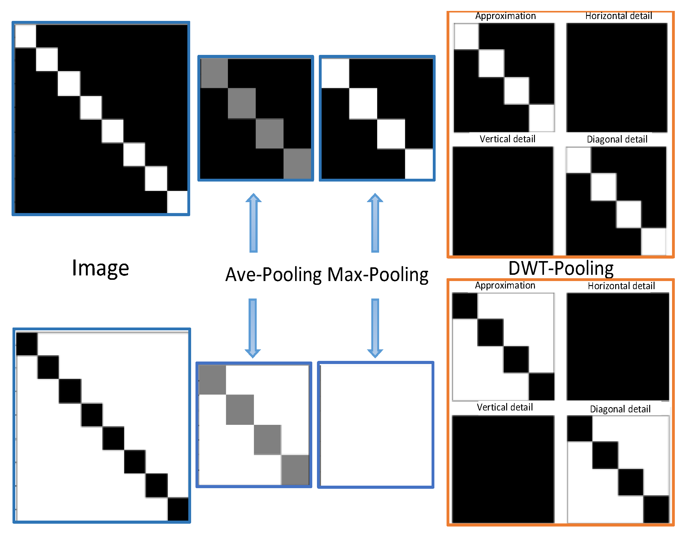
34]. Average pooling, depending on the data, can dilute the relevant details of an image. Averaging data with values far below important details cause this action [
9].
Figure 1 illustrates these shortcomings with the example of a toy image.
If we consider DWT filters as convolutional filters with predefined weights, then we can observe that DWT is a particular case of FCN (Fully Connected Layers) without the layers of nonlinearity. The original image can be decomposed by DWT and then reconstructed exactly by the DWT inverse without losing information [
18]. On the other hand, the wavelet theory opens the possibility to represent the image details inside learning CNNs, thanks to the frequency and location features generated by the wavelet transform (see
Figure 1 [
17]).
3.2. Network Training and Parameter Setting
The algorithms are implemented and developed using the Python language and Keras API with Tensorflow as Backend. Keras is one of the deep learning frameworks with tools to create classification models. Moreover, it is an open-source project, and its manner of programming is sequential through blocks [
35]. The hardware specifications of the training device are an Intel
® Core™ i7 processor with an NVIDIA GeForce RTX™ 2080 graphics card, 12 GB of RAM, and Ubuntu 18.04 64-bit operating system.
The base architecture is the VGG network, and it is one of the first deep models with good results in a large-scale visual recognition challenge (ILSVRC-2014) with 92.7% top-5 accuracy [
36]. This architecture is designed to facilitate the creation of a
classification model—three convolutional blocks with their pooling layer and one classification stage. The process is as follows: using the base VGG architecture, combined with the preprocessed CIFAR-10, DTD, and FMD datasets, through supervised learning. Before training our CNN, the loss function and the optimizer need to be specified. These parameters determine how the network weights should be updated during the training process. In order to compile the network with Keras, we use the compile() function. Training a CNN means finding the best set of weights to map the inputs (
images) to the outputs (
labels) in the training dataset and, at the same time, in the validation dataset. Training is processed over epochs. An epoch is an iteration through all samples of the training dataset. Moreover, it is common for an epoch to be split into minibatches. Each minibatch consists of one or more samples. After each batch iteration, the weights of the network will be updated. In order to train the network with Keras, we use the fit() function. The training parameters for the proposed models are listed in
Table 1.
We perform a complete analysis with each of the proposed pooling methods: MaxP, AveP, DWTP, DWTaP, and DWTdP. In addition, we combine them with the regularization methods DropOut [
37,
38], Data Augmentation [
17,
39], and Batch Normalization [
40,
41]. In this manner, a learning model is obtained, and we can predict the objects, textures, and materials in the dataset (test) images with better accuracy.
3.3. Benchmark Dataset
In classification tasks, the model must be evaluated on a dataset. We have performed our experiments on three datasets. The first dataset is CIFAR-10 [
42], the second one is the Describable Textures Dataset (DTD) [
43], and the last one is Flickr Material Database (FMD) [
44]. CIFAR-10 consists of 60,000 images of 32 × 32 pixels of ten different objects. DTD contains 47 classes of 120 images in the wild. This dataset is developed in different uncontrolled conditions. Initially, it includes 40 training images, 40 validation images, and 40 test images for each class. Finally, FMD is built with standard materials. It has ten classes of 100 images, and each image is hand-picked from Flickr.com (under Creative Commons license) to ensure a variety of lighting conditions, compositions, colors, texture, and material subtypes.
A good practice is to split our dataset using the Hold-Out Cross-Validation sampling technique [
35]. The technique is used to test the model’s predictive performance and how well it performs on the test or unseen data. The dataset is initially separated into two sets: training and test; then, the training set is split into two subsets: training and validation. The idea is that each set contains representative images of each class. Therefore, it is achieved to have balanced sets and random. In the case of CIFAR-10, the test set is initially left with approximately 16.66%, and the training set is divided into two subsets with the same distribution of images: training 80% and validation 20%. For DTD and FMD, the distribution is different because the dataset is small. The test set contains 15% of the data. Therefore, the rest is divided into the training subset with 82% and the validation subset with 18% of the data.
The images have dimensions of 224 × 224 pixels, except for the CIFAR-10 dataset, which has dimensions of 32 × 32 pixels. Following convention, it is helpful to normalize the pixel values to a range of 0 to 1 for our model to converge quickly because the inputs with large integer values can slow down the learning process. The number of images per class is shown in
Table 2. As observed, the last two datasets have a few images, but one advantage is that they have a balance between the number of images per class.
3.4. Evaluation Index
To quantitatively evaluate the classification model based on the combination of deep neural networks with pooling methods, this paper adopts the metrics Accuracy, Recall, Precision,
F1, and the confusion matrix to evaluate the classification index [
45]. Accuracy measures the percentage of cases that the model predicted correctly. In this case, it functions well because the classes are correctly balanced. The indicators are calculated from Equations (
4)–(
7):
where
is the number of positive samples correctly predicted, and
is the number of samples where negative samples are predicted as positive.
is the number of positive samples that are predicted as negative samples. The Scikit learn library provides us with a classification report to evaluate the quality of the predictions of a classification algorithm. The method shows us the main classification metrics (
classification_report).
4. Proposed Method
The design of an effective model for texture and material classification considers several issues: CNN architecture, dataset, regularization methods, model accuracy, and information pooling. The proposed wavelet pooling method mainly focuses on improving the model’s classification performance. Moreover, the wavelet pooling method reduces the artifacts that result during a dimension reduction in feature maps. Our approach preserves the significant features that traditional methods cannot retain. To evaluate our approach (DWTP) and to have the effect of each pooling method concerning the dataset, we outline the main steps below:
We decided to involve digital images containing mainly textures and materials for the CNN training. Textures and materials are key features for evaluating the pooling method against a loss of information with repetitive patterns.
Each dataset being evaluated is divided into three parts: training, validation, and test. A higher distribution percentage for the training set and the remaining percentages for the validation and test sets are similar. This is a good practice in state-of-the-art CNNs [
35].
An approximate version of the VGG16 architecture is used in the CNN design but with only three convolutional blocks. In addition, a classification block is proposed for our research case. The training hyperparameters are described in
Table 1.
The configuration for pooling inside each convolutional block of the CNN (Block.CX) permits a reduction in the feature map. This initial configuration depends on the selection of the pooling method. Therefore, we have at our disposal Ave and Max Pooling, the proposed DWTP method, and the complementary versions DWTaP and DWTdP.
The evaluation stage includes the analysis of the classifier with the accuracy metric because it allows us to evaluate the performance of the model and its learning behavior.
Finally, we use regularization methods to improve the performance of the model.
The main contribution is to perform pooling (as a layer) inside the CNN using a level-based decomposition approach. Hence, the proposed approach (DWTP) concatenates the sub-images
,
,
and
, given Equation (
3). From this approach, we obtain two configurations. The first configuration (DWTaP) uses only the first level approximation sub-band
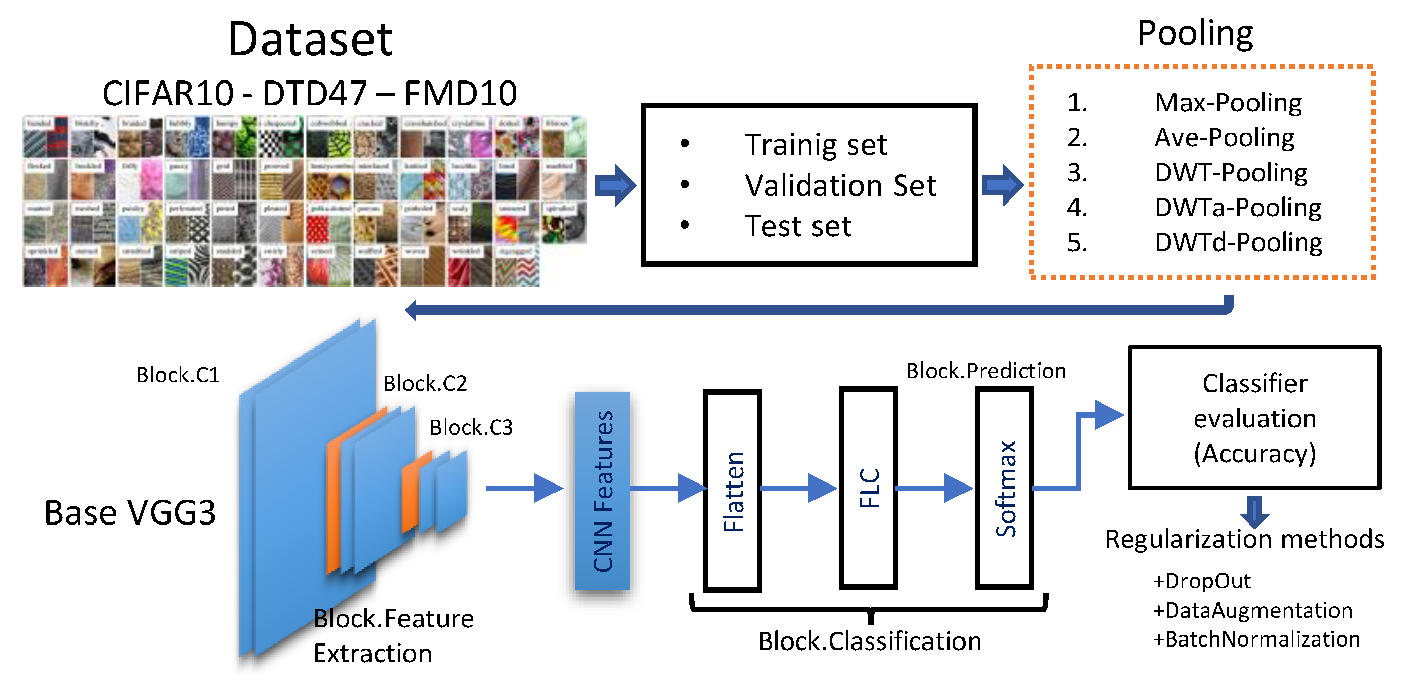
, and the second approach (DWTdP) uses all the first level detail sub-bands. The traditional methods (AveP–MaxP) are implemented with the Keras and TensorFlow methods. The diagram of the proposed methodology is presented in
Figure 2.
5. Experimental Results
The different classification models created allow us to analyze the contribution of wavelet pooling; in this case, we can analyze images with objects, textures, and materials. We can also observe the learning curve of the proposed pooling methods. Furthermore, we incorporate regularization methods for image classification to improve the model’s learning capability. The experiments obtained using the three proposed regularization techniques are shown in
Figure A1 and
Figure A2 in
Appendix A, based on the VGG architecture and the pooling method. In this manner, a complete analysis of the performance of the classifier is provided.
5.1. Model Training Results and Analysis
In order to perform efficiency testing of each pooling method on each dataset, we use an initial configuration where each pooling layer inside the architecture has only one pooling method at a time. All pooling methods use a 2 × 2 window to perform the comparison with the proposed method.
5.1.1. Image Classification CIFAR-10
The first dataset we used is CIFAR-10, with a set of 60,000 images.
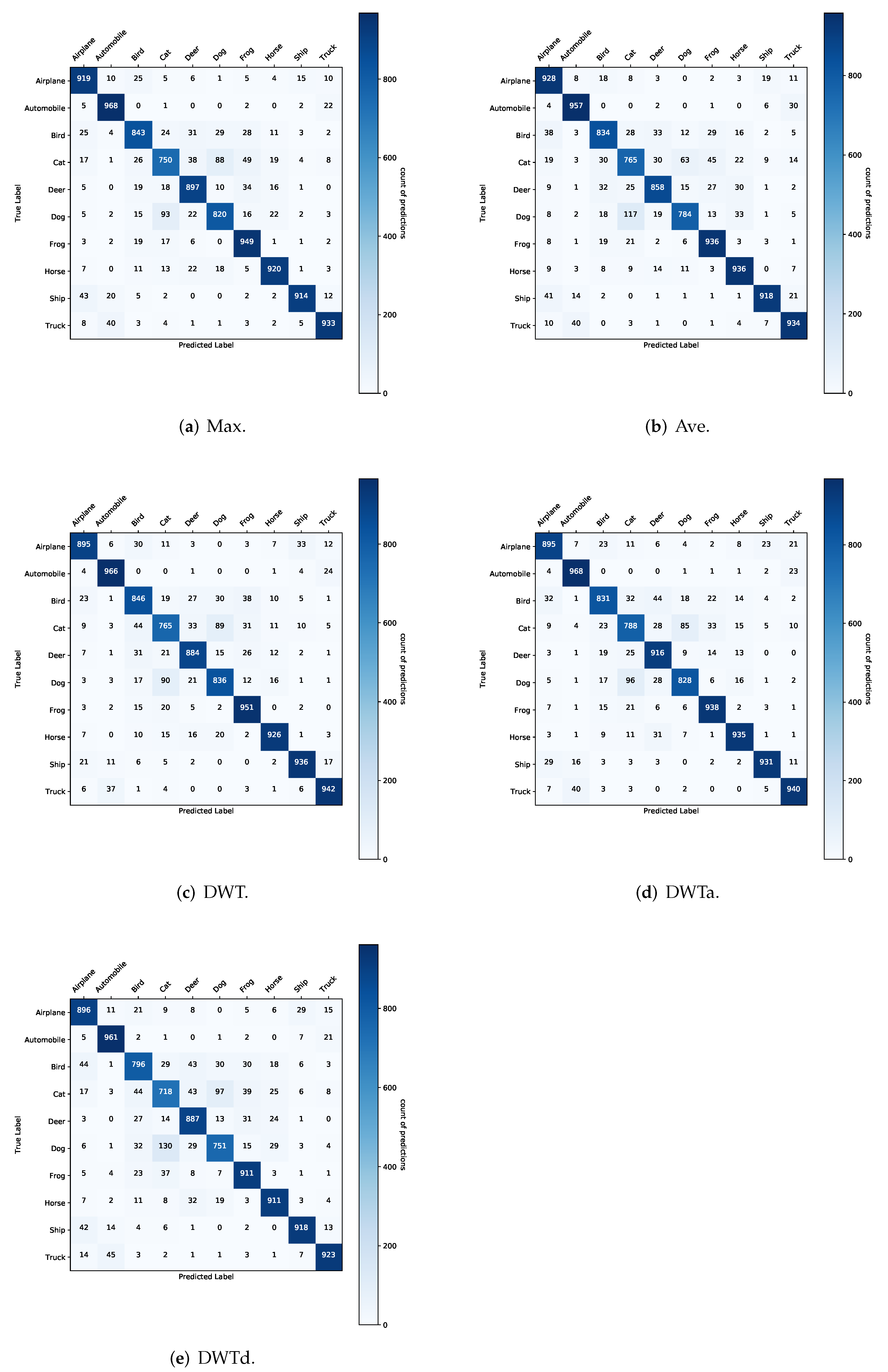
Table 3 shows that our proposed method outperforms all methods. In this sense, the DWTaP combination uses only the approximation information. In addition, we retain the number of parameters to be trained.
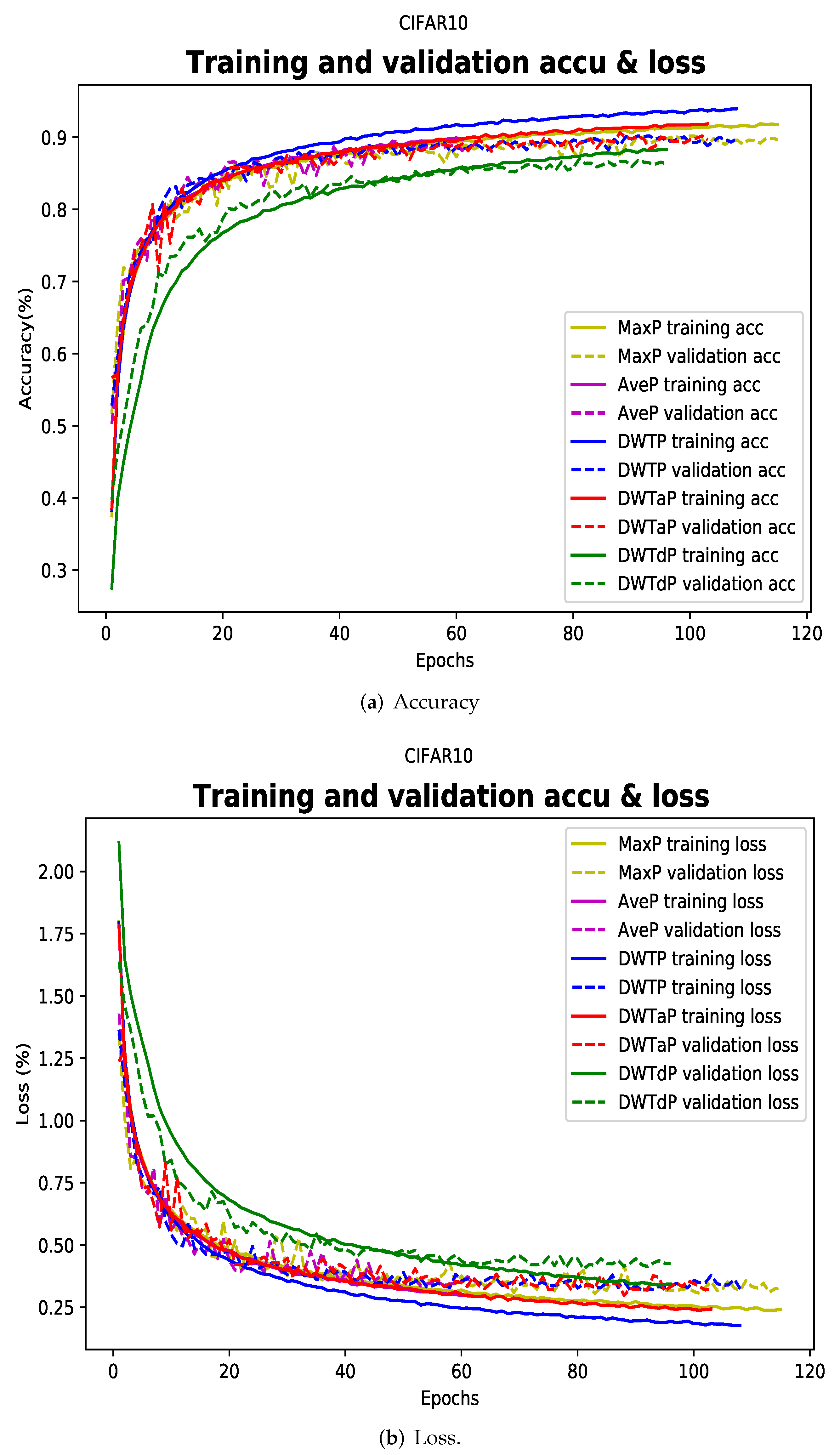
Figure 3 shows the learning curves of the pooling methods for CIFAR-10. In this case, it is observed that MaxP and DWTaP resist overfitting; moreover, it shows a slower tendency to learn in both sets. AveP maintains a consistent learning progression in both sets, but accuracy does not improve after epoch 50. In DWTP, it shows the smoothest drop-in learning. It also achieves the best accuracy performance for the training set. DWTdP shows a rapid decrease during learning, which does not resist overfitting after epoch 70.
The correlation of each class with their actual and predicted label for each model is shown in
Figure A3 in
Appendix B, which shows the multiple confusion matrix. Moreover, the classification report with the evaluation metrics for CIFAR-10 is shown in
Table A1 of
Appendix C.
5.1.2. Image Classification with Textures DTD
The second dataset we use is DTD, with 47 classes of different textures. Note that it has only 120 images for each category, which may cause overfitting in the model. Thus, the proposed method is also a solution when you have a small dataset. In this case, we performed two experiments by varying the training optimizer. First, we use SGD as the optimizer.
Table 4 shows that our proposed DWTP method using its DWTaP configuration outperforms all the methods. In addition, we retain similitude in all three sets: training (37.40%), validation (31.17%), and test (34.16%). The DWTaP model obtained with this configuration is shown in
Figure A4 of
Appendix B, which shows the correlation of each class with its actual and predicted label. Based on this result, we decided to use the following optimizer to improve classification performances.
In the second experiment, we use an Adam-an extension of stochastic gradient descent.
Table 5 shows that our proposed DWTaP method and MaxP exhibit the best classification performance on all three data sets. In this case, we consider a change in the optimizer that resulted in an essential factor for learning MaxP.
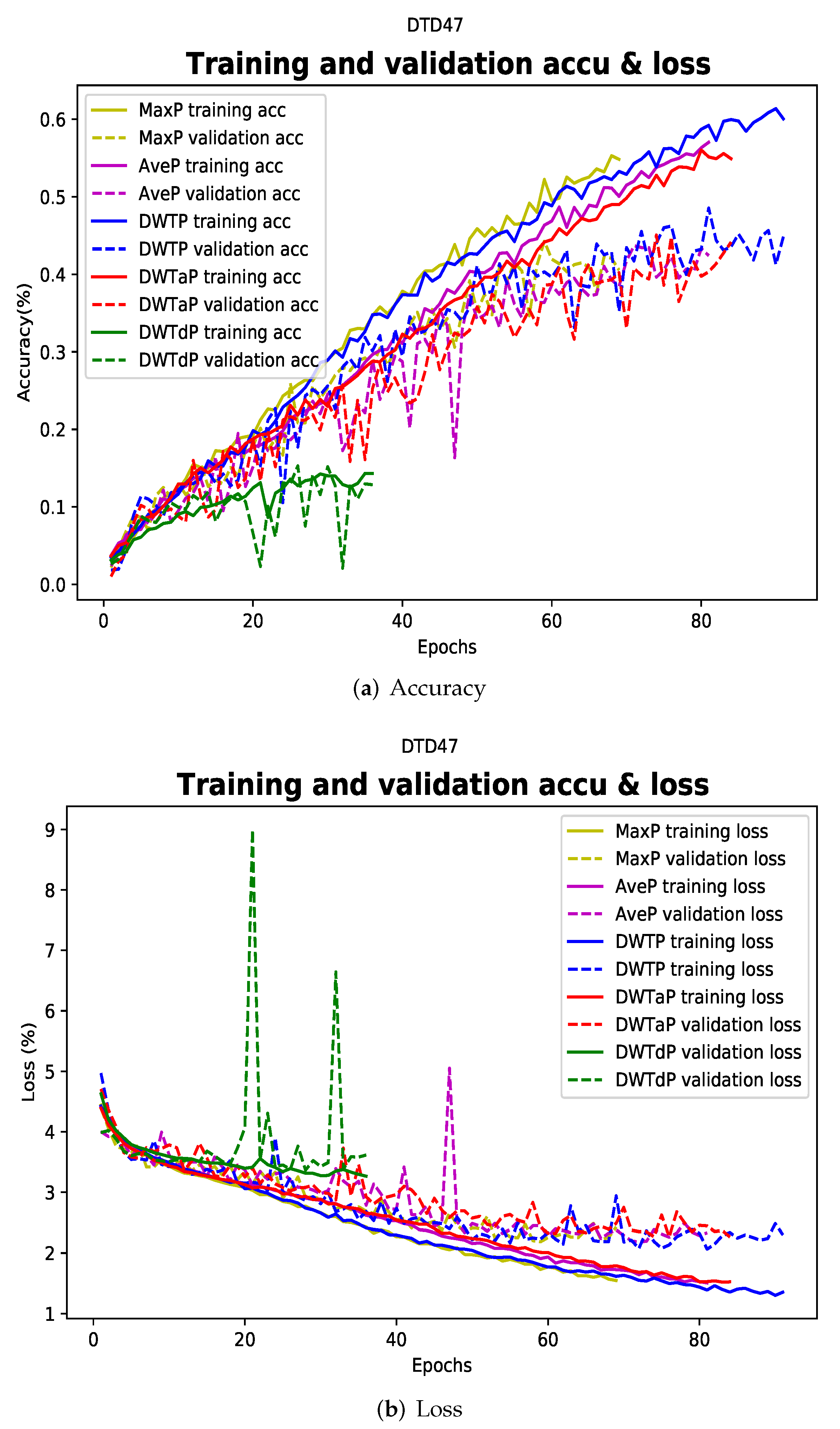
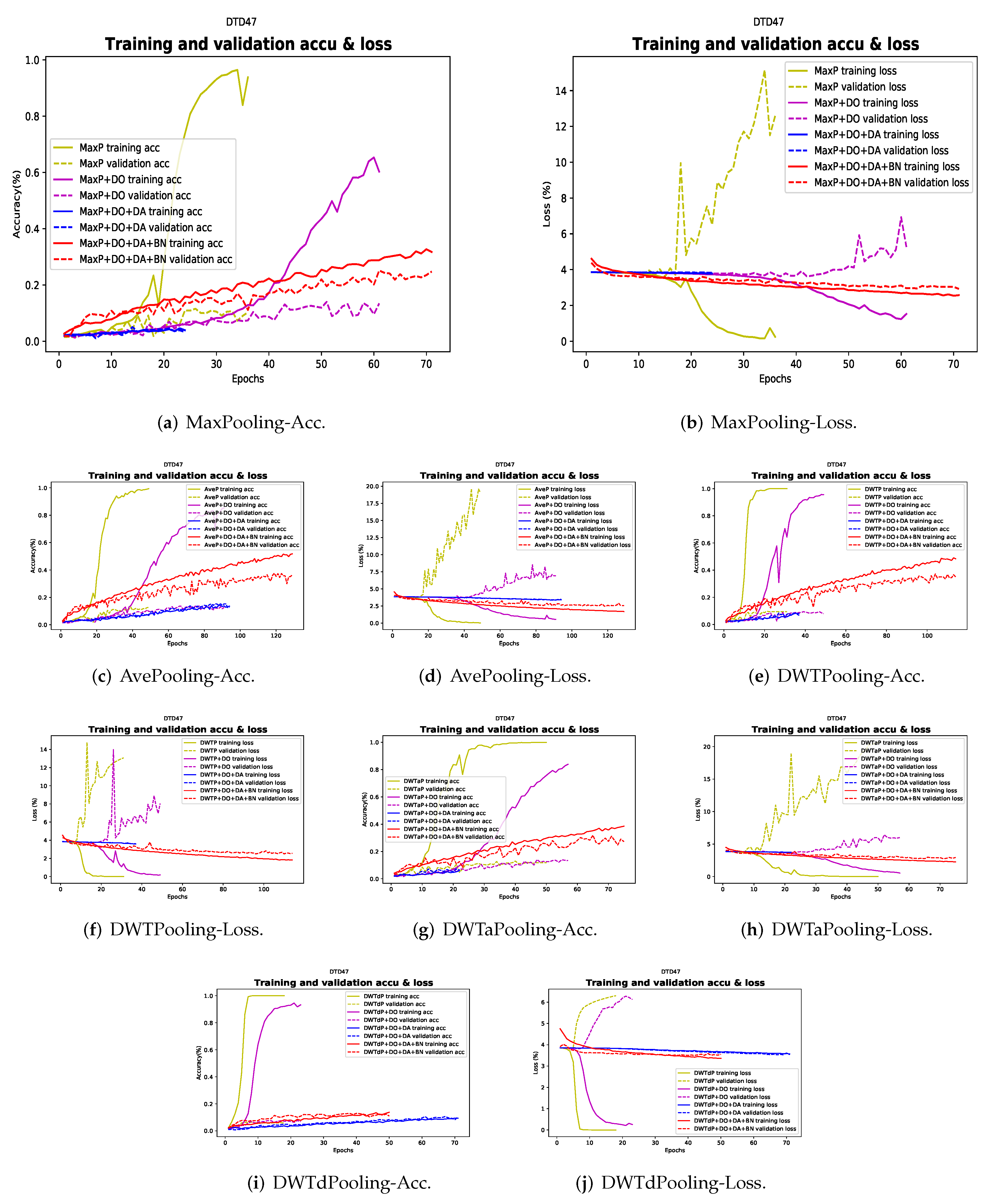
Figure 4 shows the learning curves of the pooling methods for DTD. Here, MaxP shows a smooth learning decay and similar behavior between the two sets. It also resists overfitting, managing to have good accuracy performance. AveP and DWTP maintain a consistent learning progression, and their validation sets progress at a similar rate but does not resist overfitting. The learning rate of DWTaP resists overfitting in both sets, achieving one of the best accuracy performances. DWTdP shows a slow learning behavior; thus, the learning rate does not improve after epoch 28.
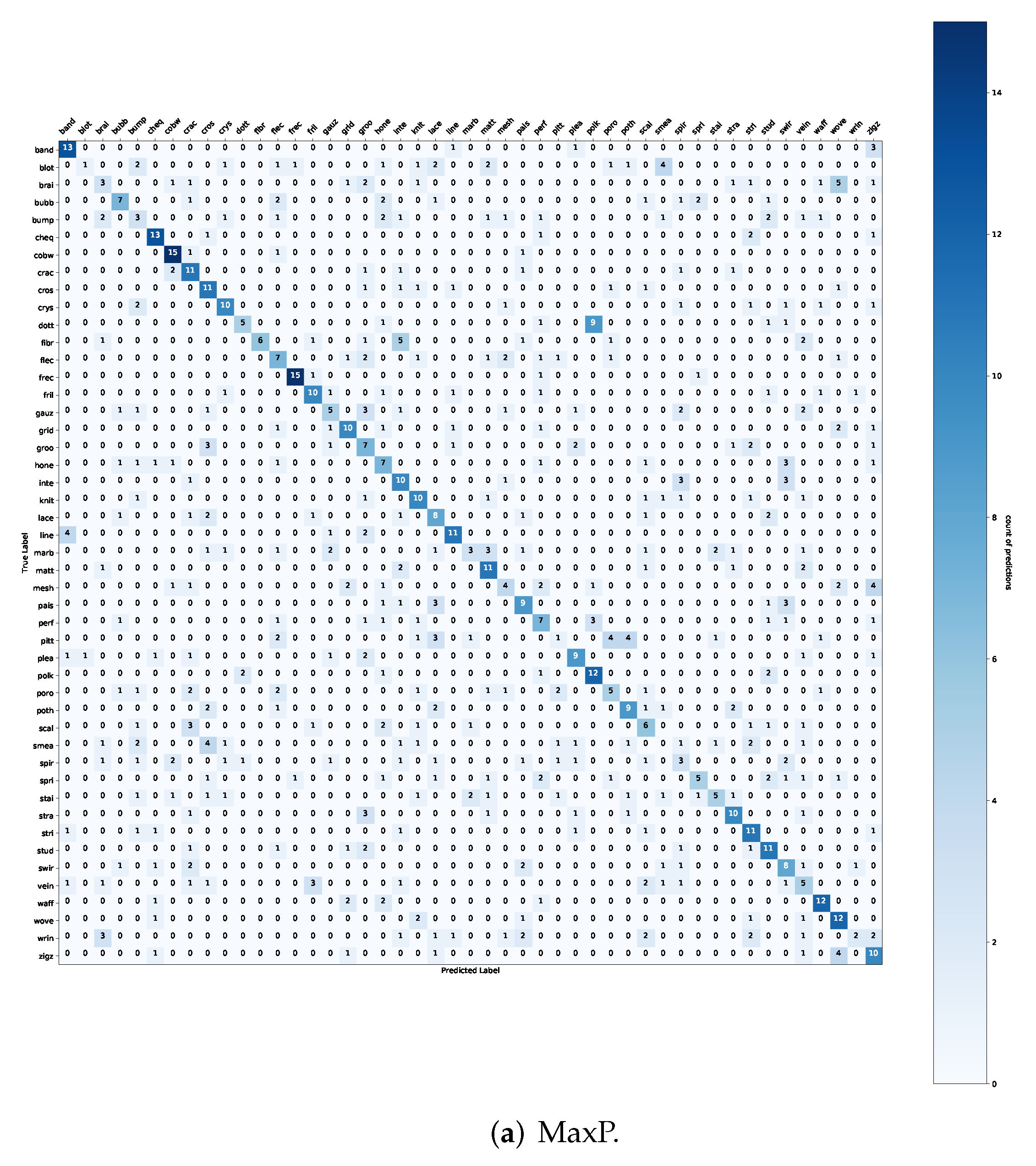
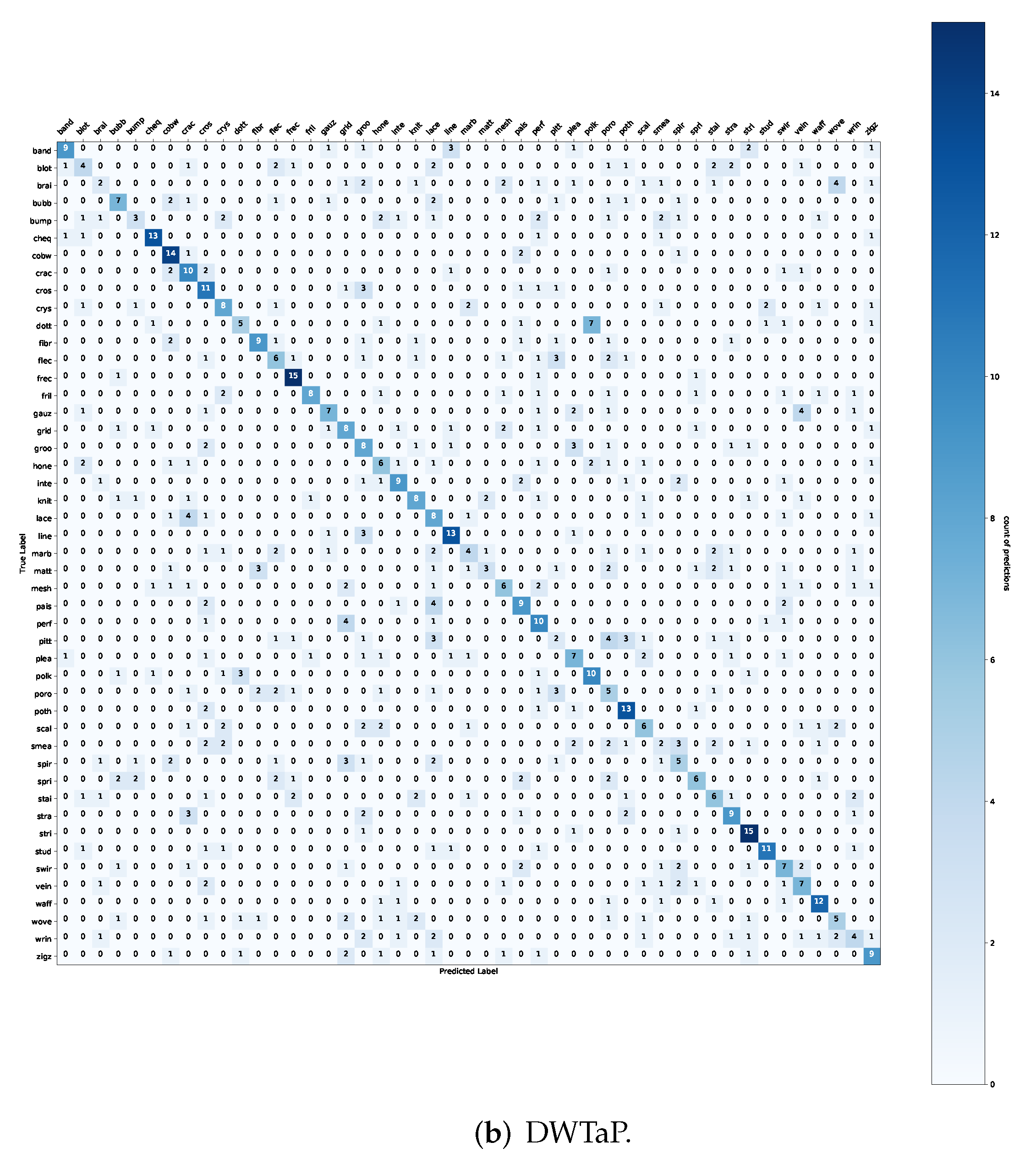
The DWTaP and MaxP learning models obtained with this configuration are shown in
Figure A5 of
Appendix B, which summarizes the level of success of the classification model predictions. Moreover, the classification reports obtained with both configurations (SGD and Adam) for DTD are shown in
Appendix C and
Table A2 and
Table A3.
5.1.3. Image Classification with Materials FMD
The third dataset we used is FMD with ten classes of different materials. Moreover, it is a small dataset since it only has 100 images per class. Likewise, we performed two experiments: the first with the SGD optimizer and the second with the Adam optimizer.
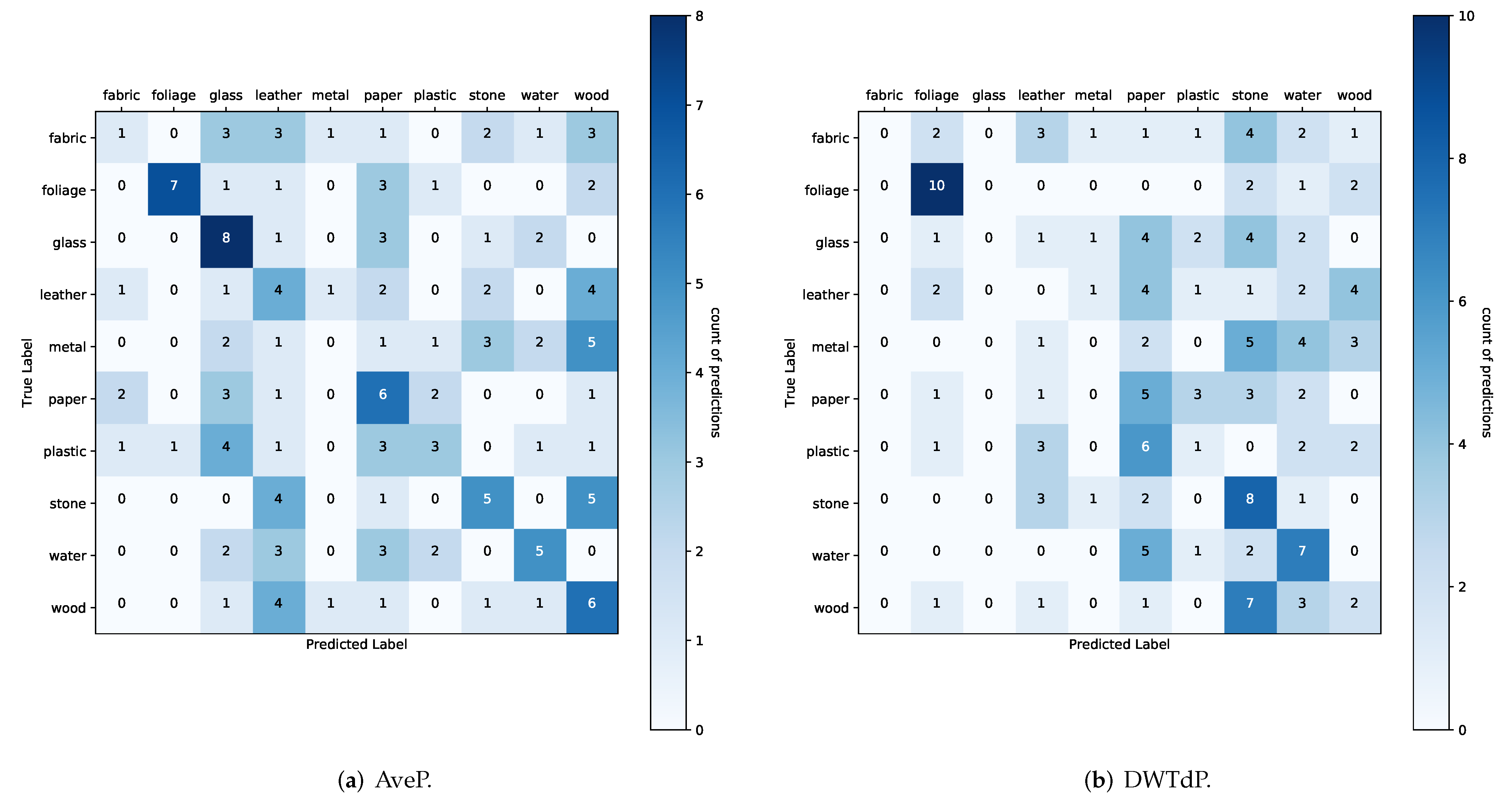
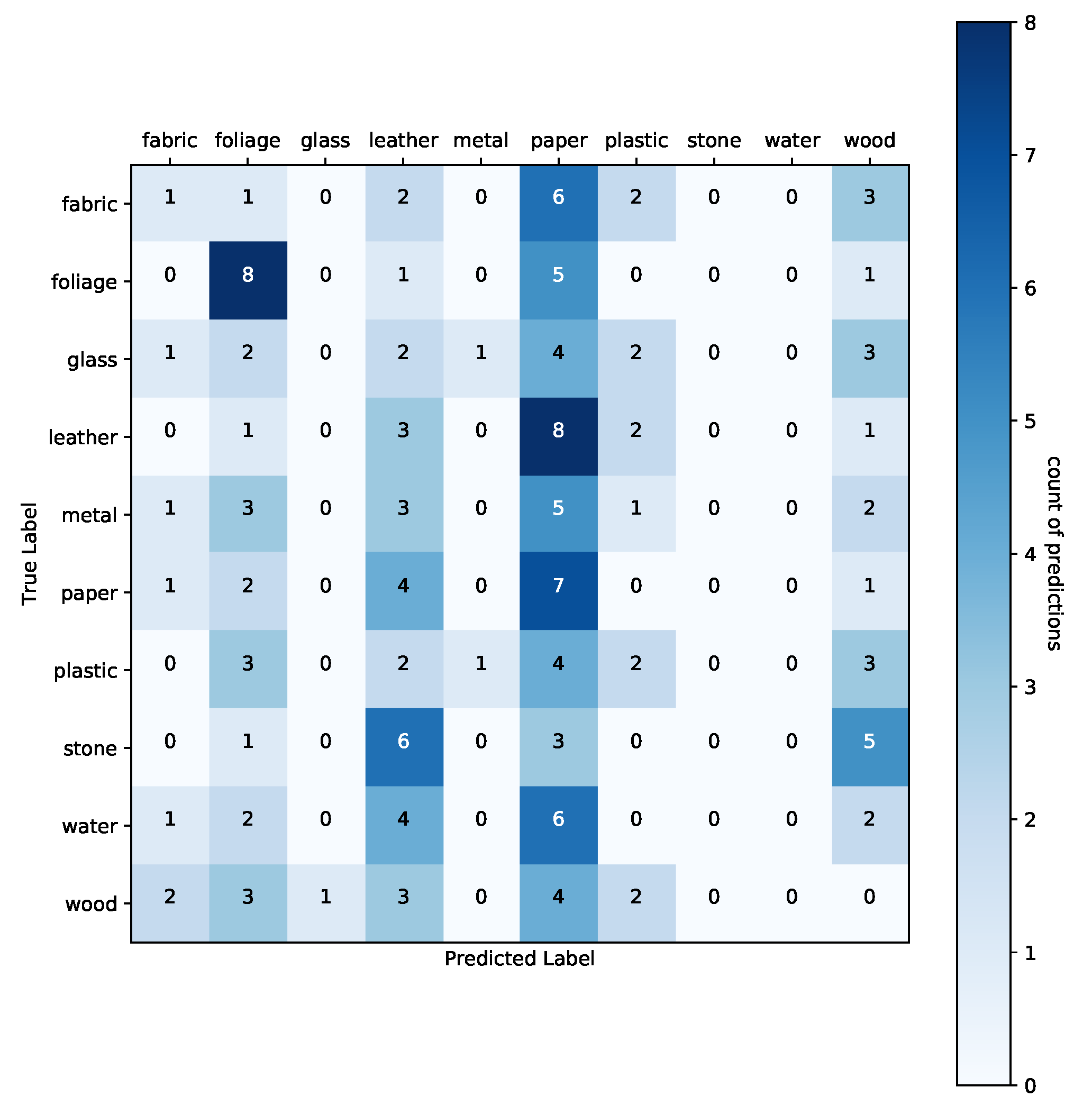
Table 6 shows that our proposed DWTP method using its DWTdP configuration outperforms all methods. In addition, we retain a similitude in the three sets: training (16.87%), validation (18.67%), and test (14.00%). The DWTdP model obtained with this configuration is shown in
Figure A6 of
Appendix B, which shows the correlation of each class with its actual and predicted label.
The change of the optimizer, in this case, was beneficial for AveP learning.
Table 7 shows that our proposed DWTdP method and AveP exhibit the best classification performance on all three datasets.
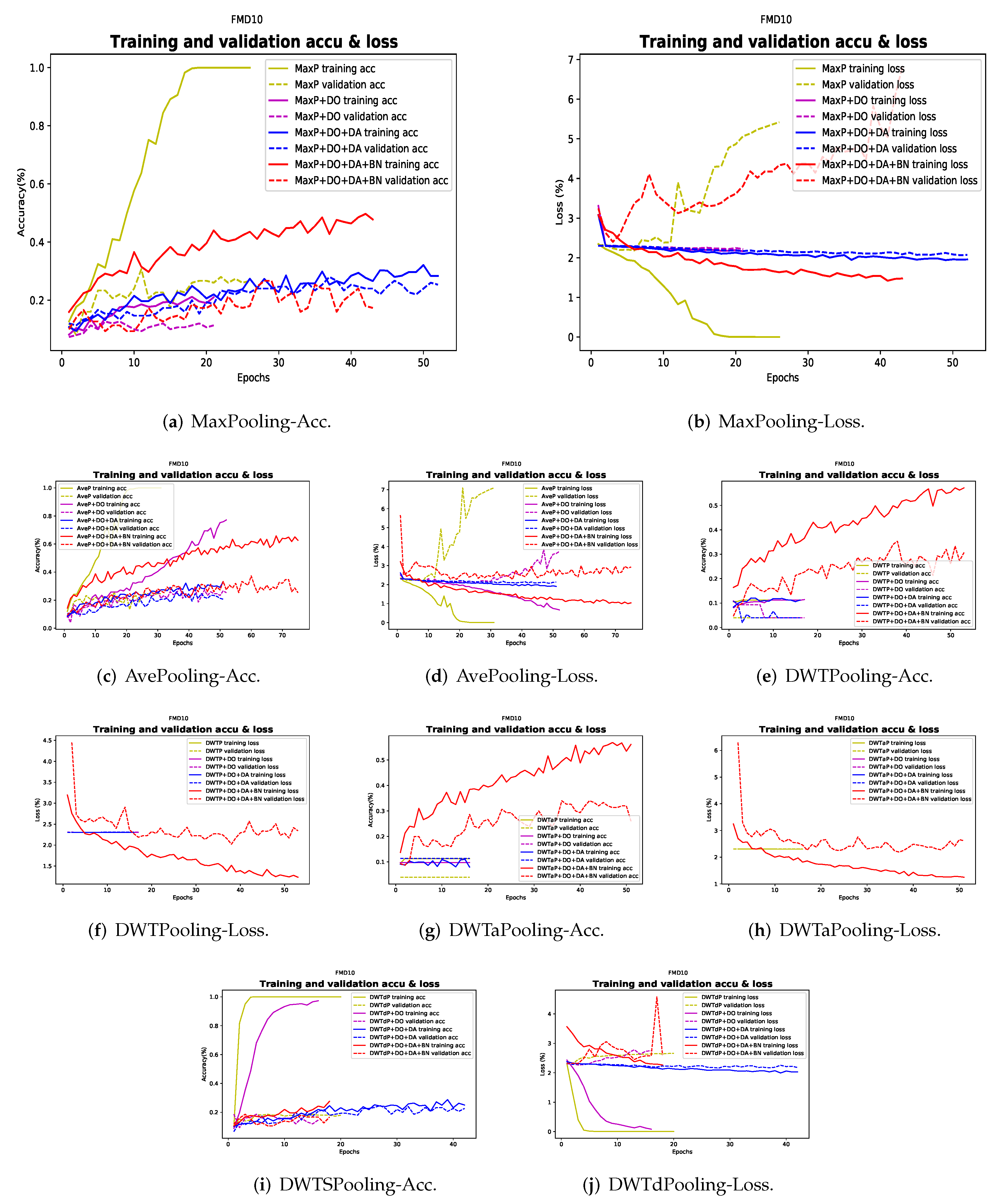
Figure 5 shows the learning curves of the pooling methods for FMD. In this case, MaxP shows a smooth learning descent and similar behavior between the two sets, but after epoch 22, it does not resist overfitting. AveP achieves the best performance at epoch 17, avoiding overfitting in the following epochs. DWTP and DWTaP maintain a consistent learning progression, and their validation sets progress at a similar rate but does not resist overfitting. DWTdP shows a slow learning trend in the early epochs, but after epoch 15, the learning rate improves, and the sets evolve at a similar rate, achieving good accuracy performance.
The DWTdP and AveP learning models obtained with this configuration are shown in
Figure A7 of
Appendix B, which summarizes the level of success of the classification model predictions. Moreover, the classification reports obtained with both configurations (SGD and Adam) for FMD are shown in
Table A4 and
Table A5 of
Appendix C.
6. Discussion
Even though CNNs have established their position in image analysis and the different elements that are considered to improve classification performance and that these are well known in the literature, only a few experiments have been conducted by taking into account the pooling layers. In
Figure 3,
Figure 4 and
Figure 5, we illustrate the learning behavior of each model and for each pooling method. From the Figures, it is clear that the DWTP versions of the model behavior in both training sets are uniformly distributed. That is, the learning curve remains stable and shows a similar generalization in all three training sets. When the optimizer change is proposed, the results are very similar for the DWTP versions. Moreover, it achieves increased classification performance for both the proposed version and the traditional methods.
Furthermore,
Table 8 contains the results of comparison of our proposals with other methods proposed by Fujieda et al. [
7] and Andrearczyk et al. [
8], where the accuracy rate for the models trained from scratch on the DTD dataset is evaluated. The bold values shown in
Table 8 indicate that our results are quite comparable with those of the other methods. Moreover, it shows the number of synaptic weights to be trained. The results show that our proposals are computationally lightweight. In a general manner, we can observe the algorithm’s efficiency for CIFAR-10 in
Table 3. Currently, this dataset can be compared in the literature because it is one of the most important in the Deep Learning area. As for FMD, we can mention that there are algorithms with a performance above that obtained; however, it differs from the central concept in combining both approaches and considering the wavelet pooling method.
On the other hand,
Table 4,
Table 5,
Table 6 and
Table 7 show that the loss metric achieves a high index in the training sets compared to
Table 3; this learning behavior is because the sets being evaluated are different. In this case, we have a CIFAR-10 with more than 1000 images per class, unlike for the sets with small data such as DTD and FMD. Therefore, the size of the dataset is one more parameter to consider for the contribution of our research, where overfitting is prevented, and we can maintain a similitude in the accuracy of the model.
In this context, it is observed that we analyzed the impact of considering DWTP and its different configurations inside CNN learning through the different experiments. Our main observations are as follows: (a) To consider a DWTP configuration in the learning stage that presents a learning uniformity; (b) the use of a DWTP configuration to reduce the number of features is desirable to preserve relevant information; and (c) although some tests upon optimizer change have a good response towards other methods, the DWTP method also increases its classification performance. However, we note that this approach depends on the dataset’s type.
7. Conclusions
We have presented wavelet pooling (DWTP, DWTaP, and DWTdP), a pooling method capable of preserving useful information to improve the classification performance of textures and materials in images. Wavelet pooling is introduced inside the proposed VGG architecture as a layer. This layer performs the same function as the traditional methods; however, the difference is that instead of using a subsampling technique on neighborhood regions, this technique is based on the multilevel decomposition of the input image using wavelet analysis. As a result, four new subsets of features contribute to model learning: approximation, vertical details, diagonal details, and horizontal details.
We demonstrate that the wavelet pooling method achieves acceptable classification performance. Moreover, wavelet pooling achieves matching and outperforms some traditional methods used in CNN learning. Our proposed method outperforms all others on the CIFAR-10 dataset with 89.70% on the test set. The DTD dataset shares a similar performance when changing the optimizer with 43%. In the case of the FMD set, the performance achieved was 22% in the detailed version and 30% with the Ave method, possessing similarities in its three training sets. The integration of DropOut, Data Augmentation, and Batch Normalization also positively reacts to the proposed methods, improving the classification performance.
The proposed methodology in its decomposition stage can result in a better reduction in image features. In addition, sub-bands at different levels can be considered in learning and could result in better accuracy. The results show that some methods perform better than others depending on the dataset, hyperparameter configurations, and the design of the CNN architecture.
On the other hand, CNN is characterized by the random aspect in the election of filters of the convolution layers. Therefore, as a further investigation, we can add stability in the selected filters inside the pooling layer.
This approach will allow us in the future to test other texture features and change the wavelet base to analyze which base works best for pooling. Moreover, the proposed architecture and pooling method can be applied in pattern recognition, classification tasks, and object detection in aerial robotics. Therefore, this is ideal for designing an object classification system for aerial navigation, where the main feature is the analysis of repetitive patterns such as textures. Furthermore, we will investigate possible methods to improve the architecture in order to reduce computational costs while preserving classification performances.
Author Contributions
Conceptualization, M.T.R.-T.; data curation, J.M.F.-C.; formal analysis, J.M.F.-C.; investigation, J.M.F.-C. and M.T.R.-T.; methodology, J.M.F.-C. and M.T.R.-T.; project administration, M.M.-C.; software, J.M.F.-C.; supervision, M.T.R.-T., M.M.-C., J.S.M., J.M.-C. and C.S.-M.; validation, M.M.-C. and J.M.-C.; writing—original draft, J.M.F.-C., M.T.R.-T. and M.M.-C.; writing—review and editing, J.S.M., J.M.-C., C.S.-M. and C.A.G.-G. All authors have read and agreed to the published version of the manuscript.
Funding
This research was supported by CONACYT through grant “Convocatoria de Ciencia Básica y Ciencia de Frontera 2022”, project ID 320036, and project CB 2017–2018 A1-S-45697.
Institutional Review Board Statement
Not applicable.
Informed Consent Statement
Not applicable.
Data Availability Statement
Not applicable.
Acknowledgments
The first author is thankful toward Consejo Nacional de Ciencia y Tecnología (CONACYT) for scholarship No. 776118.
Conflicts of Interest
The authors declare no conflict of interest.
Abbreviations
The following abbreviations are used in this manuscript:
| CNN | Convolutional Neural Network |
| DWTP | Discrete Wavelet Transform Pooling |
| 2DWT | Two-Dimensional Wavelet Transform |
| DWTaP | Discrete Wavelet Transform Approximation Pooling |
| DWTdP | Discrete Wavelet Transform Details Pooling |
| DTD | Describable Textures Dataset |
| FMD | Flickr Material Database |
Appendix A. Training Process Using Regularization Techniques and Pooling
Appendix A.1. DTD Dataset
Figure A1.
Learning behavior for baseline architecture + pooling, increasing DropOut, Data Augmentation, and Batch Normalization—DTD dataset.
Figure A1.
Learning behavior for baseline architecture + pooling, increasing DropOut, Data Augmentation, and Batch Normalization—DTD dataset.
Appendix A.2. FMD Dataset
Figure A2.
Learning behavior for baseline architecture + pooling, increasing DropOut, Data Augmentation, and Batch Normalization—FMD dataset.
Figure A2.
Learning behavior for baseline architecture + pooling, increasing DropOut, Data Augmentation, and Batch Normalization—FMD dataset.
Appendix B. Multiple Confusion Matrix
The multiple confusion matrix is an table that summarizes the level of success in the predictions of a classification model: that is, the correlation between the label and the classification of the model.
Appendix B.1. CIFAR-10 Dataset
Figure A3.
In this case, each confusion matrix correlates with the five models obtained for the CIFAR-10 dataset.
Figure A3.
In this case, each confusion matrix correlates with the five models obtained for the CIFAR-10 dataset.
Appendix B.2. DTD Dataset
Figure A4.
Experiment 1 with SGD Optimizer—the confusion matrix correlates with the best model (DWTaP) obtained for the DTD dataset.
Figure A4.
Experiment 1 with SGD Optimizer—the confusion matrix correlates with the best model (DWTaP) obtained for the DTD dataset.
Figure A5.
Experiment 2 with Adam Optimizer—the confusion matrix correlates with the two best models (MaxP and DWTaP) for the DTD dataset.
Figure A5.
Experiment 2 with Adam Optimizer—the confusion matrix correlates with the two best models (MaxP and DWTaP) for the DTD dataset.
Appendix B.3. FMD Dataset
Figure A6.
Experiment 1 with SGD Optimizer—The confusion matrix correlates with the best model (DWTdP) obtained for the FMD dataset.
Figure A6.
Experiment 1 with SGD Optimizer—The confusion matrix correlates with the best model (DWTdP) obtained for the FMD dataset.
Figure A7.
Experiment 2 with Adam Optimizer—the confusion matrix correlates with the two best models (AveP and DWTdP) for the DTD dataset.
Figure A7.
Experiment 2 with Adam Optimizer—the confusion matrix correlates with the two best models (AveP and DWTdP) for the DTD dataset.
Appendix C. Classification Report with Evaluation Metrics
Appendix C.1. CIFAR-10 Dataset
Table A1.
Classification report for CIFAR-10 dataset. In this case, each pooling method is evaluated considering DropOut, Data Augmentation, and Batch Normalization.
Table A1.
Classification report for CIFAR-10 dataset. In this case, each pooling method is evaluated considering DropOut, Data Augmentation, and Batch Normalization.
| Method | MaxP | AveP | DWTP | DWTaP | DWTdP | |
|---|
| Class | P | R | F1 | P | R | F1 | P | R | F1 | P | R | F1 | P | R | F1 | Test |
| airplane | 0.89 | 0.92 | 0.90 | 0.86 | 0.93 | 0.89 | 0.92 | 0.90 | 0.90 | 0.90 | 0.90 | 0.90 | 0.86 | 0.90 | 0.88 | 1000 |
| automobile | 0.92 | 0.97 | 0.95 | 0.93 | 0.96 | 0.94 | 0.94 | 0.97 | 0.95 | 0.93 | 0.97 | 0.95 | 0.92 | 0.96 | 0.94 | 1000 |
| bird | 0.87 | 0.84 | 0.86 | 0.87 | 0.83 | 0.85 | 0.85 | 0.85 | 0.85 | 0.88 | 0.83 | 0.86 | 0.83 | 0.80 | 0.81 | 1000 |
| cat | 0.81 | 0.75 | 0.78 | 0.78 | 0.77 | 0.77 | 0.81 | 0.77 | 0.78 | 0.80 | 0.79 | 0.79 | 0.75 | 0.72 | 0.73 | 1000 |
| deer | 0.88 | 0.90 | 0.89 | 0.89 | 0.86 | 0.87 | 0.89 | 0.88 | 0.89 | 0.86 | 0.92 | 0.89 | 0.84 | 0.89 | 0.86 | 1000 |
| dog | 0.85 | 0.82 | 0.83 | 0.88 | 0.78 | 0.83 | 0.84 | 0.84 | 0.84 | 0.86 | 0.83 | 0.84 | 0.82 | 0.75 | 0.78 | 1000 |
| frog | 0.87 | 0.95 | 0.91 | 0.88 | 0.78 | 0.83 | 0.89 | 0.95 | 0.92 | 0.92 | 0.94 | 0.93 | 0.88 | 0.91 | 0.89 | 1000 |
| horse | 0.92 | 0.92 | 0.92 | 0.88 | 0.94 | 0.91 | 0.94 | 0.93 | 0.93 | 0.93 | 0.94 | 0.93 | 0.90 | 0.91 | 0.90 | 1000 |
| ship | 0.96 | 0.91 | 0.94 | 0.95 | 0.92 | 0.93 | 0.94 | 0.94 | 0.94 | 0.95 | 0.93 | 0.94 | 0.94 | 0.92 | 0.93 | 1000 |
| truck | 0.94 | 0.93 | 0.94 | 0.91 | 0.93 | 0.92 | 0.94 | 0.94 | 0.94 | 0.93 | 0.94 | 0.93 | 0.93 | 0.92 | 0.93 | 1000 |
| Acc | | | 0.89 | | | 0.89 | | | 0.89 | | | 0.90 | | | 0.87 | 10,000 |
Appendix C.2. DTD Dataset
Table A2.
Experiment 1 with SGD Optimizer—classification report for the DTD dataset.
Table A2.
Experiment 1 with SGD Optimizer—classification report for the DTD dataset.
| Method | MaxP | AveP | DWTP | DWTaP | DWTdP | |
|---|
| Class | P | R | F1 | P | R | F1 | P | R | F1 | P | R | F1 | P | R | F1 | Test |
| band | 0.67 | 0.44 | 0.53 | 0.75 | 0.50 | 0.60 | 0.71 | 0.56 | 0.63 | 0.83 | 0.56 | 0.67 | 0.12 | 0.06 | 0.08 | 18 |
| blot | 0.00 | 0.00 | 0.00 | 0.33 | 0.06 | 0.10 | 0.08 | 0.06 | 0.06 | 0.13 | 0.11 | 0.12 | 0.00 | 0.00 | 0.00 | 18 |
| brai | 0.17 | 0.06 | 0.08 | 0.13 | 0.11 | 0.12 | 0.29 | 0.11 | 0.16 | 0.10 | 0.06 | 0.07 | 0.11 | 0.06 | 0.07 | 18 |
| bubb | 0.17 | 0.06 | 0.08 | 0.64 | 0.39 | 0.48 | 0.30 | 0.33 | 0.32 | 0.20 | 0.17 | 0.18 | 0.10 | 0.11 | 0.11 | 18 |
| bump | 0.73 | 0.44 | 0.55 | 0.43 | 0.17 | 0.24 | 0.00 | 0.00 | 0.00 | 1.00 | 0.17 | 0.29 | 0.00 | 0.00 | 0.00 | 18 |
| cheq | 0.48 | 0.67 | 0.56 | 0.75 | 0.50 | 0.60 | 0.65 | 0.61 | 0.63 | 0.69 | 0.50 | 0.58 | 0.33 | 0.33 | 0.33 | 18 |
| cobw | 0.48 | 0.67 | 0.56 | 0.68 | 0.72 | 0.70 | 0.52 | 0.72 | 0.60 | 0.61 | 0.61 | 0.61 | 0.12 | 0.06 | 0.08 | 18 |
| crac | 0.45 | 0.28 | 0.34 | 0.33 | 0.44 | 0.38 | 0.33 | 0.44 | 0.38 | 0.29 | 0.33 | 0.31 | 0.11 | 0.11 | 0.11 | 18 |
| cros | 0.16 | 0.44 | 0.24 | 0.36 | 0.56 | 0.43 | 0.24 | 0.50 | 0.33 | 0.27 | 0.67 | 0.38 | 0.00 | 0.00 | 0.00 | 18 |
| crys | 0.35 | 0.33 | 0.34 | 0.60 | 0.50 | 0.55 | 0.53 | 0.44 | 0.48 | 0.29 | 0.33 | 0.31 | 0.11 | 0.11 | 0.11 | 18 |
| dott | 0.80 | 0.22 | 0.35 | 0.15 | 0.11 | 0.13 | 0.42 | 0.28 | 0.33 | 0.50 | 0.28 | 0.36 | 0.00 | 0.00 | 0.00 | 18 |
| fibr | 0.17 | 0.28 | 0.21 | 0.41 | 0.39 | 0.40 | 0.35 | 0.44 | 0.39 | 0.30 | 0.39 | 0.34 | 0.12 | 0.33 | 0.18 | 18 |
| flec | 0.15 | 0.44 | 0.22 | 0.13 | 0.39 | 0.19 | 0.18 | 0.17 | 0.17 | 0.17 | 0.56 | 0.26 | 0.10 | 0.17 | 0.13 | 18 |
| frec | 0.43 | 0.56 | 0.49 | 0.64 | 0.78 | 0.70 | 0.93 | 0.78 | 0.85 | 0.50 | 0.72 | 0.59 | 0.21 | 0.67 | 0.32 | 18 |
| fril | 0.21 | 0.22 | 0.22 | 0.53 | 0.44 | 0.48 | 0.60 | 0.50 | 0.55 | 0.36 | 0.28 | 0.31 | 0.00 | 0.00 | 0.00 | 18 |
| gauz | 0.38 | 0.17 | 0.23 | 0.32 | 0.33 | 0.32 | 0.39 | 0.39 | 0.39 | 0.45 | 0.28 | 0.34 | 0.10 | 0.22 | 0.14 | 18 |
| grid | 0.14 | 0.06 | 0.08 | 0.36 | 0.44 | 0.40 | 0.40 | 0.56 | 0.47 | 0.40 | 0.56 | 0.47 | 0.00 | 0.00 | 0.00 | 18 |
| groo | 0.18 | 0.33 | 0.23 | 0.17 | 0.39 | 0.24 | 0.32 | 0.61 | 0.42 | 0.22 | 0.44 | 0.29 | 0.00 | 0.00 | 0.00 | 18 |
| hone | 0.50 | 0.06 | 0.10 | 0.50 | 0.17 | 0.25 | 0.42 | 0.28 | 0.33 | 0.00 | 0.00 | 0.00 | 0.00 | 0.00 | 0.00 | 18 |
| inte | 0.36 | 0.28 | 0.31 | 0.40 | 0.44 | 0.42 | 0.38 | 0.44 | 0.41 | 0.83 | 0.28 | 0.42 | 0.17 | 0.06 | 0.08 | 18 |
| knit | 0.13 | 0.50 | 0.21 | 0.43 | 0.56 | 0.49 | 0.57 | 0.44 | 0.50 | 0.25 | 0.56 | 0.34 | 0.00 | 0.00 | 0.00 | 18 |
| lace | 0.14 | 0.28 | 0.18 | 0.29 | 0.33 | 0.31 | 0.22 | 0.44 | 0.30 | 0.24 | 0.72 | 0.36 | 0.07 | 0.17 | 0.10 | 18 |
| line | 0.41 | 0.72 | 0.52 | 0.52 | 0.67 | 0.59 | 0.53 | 0.56 | 0.54 | 0.71 | 0.56 | 0.63 | 0.11 | 0.06 | 0.07 | 18 |
| marb | 0.21 | 0.33 | 0.26 | 0.43 | 0.33 | 0.38 | 0.23 | 0.28 | 0.25 | 0.25 | 0.17 | 0.20 | 0.06 | 0.11 | 0.07 | 18 |
| matt | 0.29 | 0.44 | 0.35 | 0.35 | 0.39 | 0.37 | 0.40 | 0.33 | 0.36 | 0.36 | 0.28 | 0.31 | 0.07 | 0.22 | 0.11 | 18 |
| mesh | 0.50 | 0.06 | 0.10 | 0.50 | 0.17 | 0.25 | 0.50 | 0.44 | 0.47 | 0.20 | 0.06 | 0.09 | 0.17 | 0.06 | 0.08 | 18 |
| pais | 0.19 | 0.22 | 0.21 | 0.34 | 0.72 | 0.46 | 0.31 | 0.56 | 0.40 | 0.33 | 0.44 | 0.38 | 0.50 | 0.06 | 0.10 | 18 |
| perf | 0.40 | 0.22 | 0.29 | 0.46 | 0.33 | 0.39 | 0.35 | 0.44 | 0.39 | 0.46 | 0.33 | 0.39 | 0.50 | 0.06 | 0.10 | 18 |
| pitt | 0.24 | 0.33 | 0.28 | 0.00 | 0.00 | 0.00 | 0.25 | 0.22 | 0.24 | 0.24 | 0.22 | 0.23 | 0.00 | 0.00 | 0.00 | 18 |
| plea | 0.60 | 0.17 | 0.26 | 0.30 | 0.33 | 0.32 | 0.37 | 0.56 | 0.44 | 0.75 | 0.17 | 0.27 | 0.00 | 0.00 | 0.00 | 18 |
| polk | 0.50 | 0.17 | 0.25 | 0.42 | 0.56 | 0.48 | 0.62 | 0.56 | 0.59 | 0.56 | 0.28 | 0.37 | 0.00 | 0.00 | 0.00 | 18 |
| poro | 0.05 | 0.06 | 0.05 | 0.50 | 0.28 | 0.36 | 0.13 | 0.11 | 0.12 | 0.17 | 0.22 | 0.19 | 0.07 | 0.17 | 0.10 | 18 |
| poth | 0.26 | 0.44 | 0.33 | 0.38 | 0.67 | 0.48 | 0.45 | 0.72 | 0.55 | 0.31 | 0.89 | 0.46 | 0.07 | 0.39 | 0.12 | 18 |
| scal | 0.00 | 0.00 | 0.00 | 0.33 | 0.11 | 0.17 | 0.22 | 0.11 | 0.15 | 0.00 | 0.00 | 0.00 | 0.12 | 0.06 | 0.08 | 18 |
| smea | 0.00 | 0.00 | 0.00 | 0.22 | 0.11 | 0.15 | 0.14 | 0.11 | 0.12 | 0.20 | 0.06 | 0.09 | 0.00 | 0.00 | 0.00 | 18 |
| spir | 0.50 | 0.11 | 0.18 | 0.20 | 0.11 | 0.14 | 0.30 | 0.17 | 0.21 | 0.25 | 0.22 | 0.24 | 0.36 | 0.22 | 0.28 | 18 |
| spri | 0.75 | 0.17 | 0.27 | 0.50 | 0.33 | 0.40 | 0.50 | 0.33 | 0.40 | 0.33 | 0.11 | 0.17 | 1.00 | 0.06 | 0.11 | 18 |
| stai | 0.10 | 0.17 | 0.12 | 0.17 | 0.06 | 0.08 | 0.25 | 0.17 | 0.20 | 0.22 | 0.28 | 0.24 | 0.22 | 0.33 | 0.27 | 18 |
| stra | 0.31 | 0.50 | 0.38 | 0.38 | 0.67 | 0.48 | 0.40 | 0.56 | 0.47 | 0.24 | 0.28 | 0.26 | 0.00 | 0.00 | 0.00 | 18 |
| stri | 0.81 | 0.72 | 0.76 | 0.55 | 0.67 | 0.60 | 0.73 | 0.61 | 0.67 | 0.75 | 0.67 | 0.71 | 0.25 | 0.28 | 0.26 | 18 |
| stud | 0.64 | 0.50 | 0.56 | 0.60 | 0.67 | 0.63 | 0.55 | 0.61 | 0.58 | 0.64 | 0.39 | 0.48 | 0.20 | 0.50 | 0.28 | 18 |
| swir | 0.50 | 0.11 | 0.18 | 0.29 | 0.22 | 0.25 | 0.00 | 0.00 | 0.00 | 0.00 | 0.00 | 0.00 | 0.00 | 0.00 | 0.00 | 18 |
| vein | 0.25 | 0.28 | 0.26 | 0.43 | 0.33 | 0.38 | 0.46 | 0.33 | 0.39 | 0.75 | 0.17 | 0.27 | 0.14 | 0.28 | 0.19 | 18 |
| waff | 0.55 | 0.67 | 0.60 | 0.79 | 0.61 | 0.69 | 0.52 | 0.78 | 0.62 | 0.52 | 0.67 | 0.59 | 0.25 | 0.56 | 0.34 | 18 |
| wove | 0.25 | 0.22 | 0.24 | 0.40 | 0.56 | 0.47 | 0.45 | 0.50 | 0.47 | 0.39 | 0.50 | 0.44 | 0.14 | 0.22 | 0.17 | 18 |
| wrin | 0.00 | 0.00 | 0.00 | 0.30 | 0.17 | 0.21 | 0.20 | 0.06 | 0.09 | 0.29 | 0.11 | 0.16 | 0.00 | 0.00 | 0.00 | 18 |
| zigz | 0.18 | 0.11 | 0.14 | 0.30 | 0.39 | 0.34 | 0.27 | 0.22 | 0.24 | 0.42 | 0.44 | 0.43 | 0.00 | 0.00 | 0.00 | 18 |
| Acc | | | 0.27 | | | 0.39 | | | 0.39 | | | 0.34 | | | 0.13 | 846 |
Table A3.
Experiment 2 with Adam Optimizer—classification report for the DTD dataset.
Table A3.
Experiment 2 with Adam Optimizer—classification report for the DTD dataset.
| Method | MaxP | AveP | DWTP | DWTaP | DWTdP | |
|---|
| Class | P | R | F1 | P | R | F1 | P | R | F1 | P | R | F1 | P | R | F1 | Test |
| band | 0.65 | 0.72 | 0.68 | 0.71 | 0.67 | 0.69 | 0.82 | 0.78 | 0.80 | 0.75 | 0.50 | 0.60 | 0.21 | 0.33 | 0.26 | 18 |
| blot | 0.50 | 0.06 | 0.10 | 0.10 | 0.06 | 0.07 | 0.22 | 0.11 | 0.15 | 0.33 | 0.22 | 0.27 | 0.00 | 0.00 | 0.00 | 18 |
| brai | 0.23 | 0.17 | 0.19 | 0.00 | 0.00 | 0.00 | 0.16 | 0.17 | 0.16 | 0.25 | 0.11 | 0.15 | 0.00 | 0.00 | 0.00 | 18 |
| bubb | 0.54 | 0.39 | 0.45 | 0.43 | 0.17 | 0.24 | 0.40 | 0.44 | 0.42 | 0.47 | 0.39 | 0.42 | 0.00 | 0.00 | 0.00 | 18 |
| bump | 0.18 | 0.17 | 0.17 | 0.18 | 0.11 | 0.14 | 0.25 | 0.06 | 0.09 | 0.38 | 0.17 | 0.23 | 0.00 | 0.00 | 0.00 | 18 |
| cheq | 0.65 | 0.72 | 0.68 | 0.60 | 0.67 | 0.63 | 0.93 | 0.72 | 0.81 | 0.76 | 0.72 | 0.74 | 0.42 | 0.28 | 0.33 | 18 |
| cobw | 0.65 | 0.83 | 0.73 | 0.67 | 0.89 | 0.76 | 0.61 | 0.94 | 0.74 | 0.52 | 0.78 | 0.62 | 0.29 | 0.11 | 0.16 | 18 |
| crac | 0.39 | 0.61 | 0.48 | 0.55 | 0.61 | 0.58 | 0.77 | 0.56 | 0.65 | 0.38 | 0.56 | 0.45 | 0.33 | 0.11 | 0.17 | 18 |
| cros | 0.39 | 0.61 | 0.48 | 0.23 | 0.50 | 0.31 | 0.40 | 0.44 | 0.42 | 0.34 | 0.61 | 0.44 | 0.00 | 0.00 | 0.00 | 18 |
| crys | 0.59 | 0.56 | 0.57 | 0.47 | 0.50 | 0.49 | 0.44 | 0.78 | 0.56 | 0.42 | 0.44 | 0.43 | 0.14 | 0.28 | 0.19 | 18 |
| dott | 0.62 | 0.28 | 0.38 | 0.45 | 0.28 | 0.34 | 0.36 | 0.22 | 0.28 | 0.50 | 0.28 | 0.36 | 0.00 | 0.00 | 0.00 | 18 |
| fibr | 1.00 | 0.33 | 0.50 | 0.53 | 0.50 | 0.51 | 0.65 | 0.61 | 0.63 | 0.60 | 0.50 | 0.55 | 0.09 | 0.17 | 0.12 | 18 |
| flec | 0.32 | 0.39 | 0.35 | 0.15 | 0.28 | 0.20 | 0.30 | 0.39 | 0.34 | 0.32 | 0.33 | 0.32 | 0.21 | 0.22 | 0.22 | 18 |
| frec | 0.88 | 0.83 | 0.86 | 0.74 | 0.78 | 0.76 | 0.88 | 0.83 | 0.86 | 0.68 | 0.83 | 0.75 | 0.17 | 0.44 | 0.25 | 18 |
| fril | 0.59 | 0.56 | 0.57 | 0.58 | 0.39 | 0.47 | 0.53 | 0.56 | 0.54 | 0.80 | 0.44 | 0.57 | 0.08 | 0.06 | 0.06 | 18 |
| gauz | 0.38 | 0.28 | 0.32 | 0.39 | 0.39 | 0.39 | 0.28 | 0.28 | 0.28 | 0.58 | 0.39 | 0.47 | 0.12 | 0.28 | 0.17 | 18 |
| grid | 0.56 | 0.56 | 0.56 | 0.56 | 0.56 | 0.56 | 0.41 | 0.67 | 0.51 | 0.33 | 0.44 | 0.38 | 0.00 | 0.00 | 0.00 | 18 |
| groo | 0.25 | 0.39 | 0.30 | 0.32 | 0.50 | 0.39 | 0.37 | 0.39 | 0.38 | 0.27 | 0.44 | 0.33 | 0.00 | 0.00 | 0.00 | 18 |
| hone | 0.29 | 0.39 | 0.33 | 0.47 | 0.44 | 0.46 | 0.24 | 0.28 | 0.26 | 0.33 | 0.33 | 0.33 | 0.00 | 0.00 | 0.00 | 18 |
| inte | 0.36 | 0.56 | 0.43 | 0.41 | 0.39 | 0.40 | 0.50 | 0.67 | 0.57 | 0.53 | 0.50 | 0.51 | 0.25 | 0.06 | 0.09 | 18 |
| knit | 0.45 | 0.56 | 0.50 | 0.36 | 0.67 | 0.47 | 0.50 | 0.50 | 0.50 | 0.50 | 0.44 | 0.47 | 0.17 | 0.28 | 0.21 | 18 |
| lace | 0.33 | 0.44 | 0.38 | 0.37 | 0.39 | 0.38 | 0.50 | 0.56 | 0.53 | 0.24 | 0.44 | 0.31 | 0.12 | 0.39 | 0.19 | 18 |
| line | 0.65 | 0.61 | 0.63 | 0.57 | 0.72 | 0.63 | 0.72 | 0.72 | 0.72 | 0.62 | 0.72 | 0.67 | 0.44 | 0.39 | 0.41 | 18 |
| marb | 0.43 | 0.17 | 0.24 | 0.26 | 0.28 | 0.27 | 0.43 | 0.33 | 0.38 | 0.36 | 0.22 | 0.28 | 0.10 | 0.17 | 0.12 | 18 |
| matt | 0.48 | 0.61 | 0.54 | 0.41 | 0.39 | 0.40 | 0.57 | 0.44 | 0.50 | 0.50 | 0.17 | 0.25 | 0.08 | 0.28 | 0.12 | 18 |
| mesh | 0.33 | 0.22 | 0.27 | 0.43 | 0.33 | 0.38 | 0.55 | 0.33 | 0.41 | 0.43 | 0.33 | 0.38 | 0.20 | 0.11 | 0.14 | 18 |
| pais | 0.45 | 0.50 | 0.47 | 0.41 | 0.72 | 0.52 | 0.48 | 0.67 | 0.56 | 0.43 | 0.50 | 0.46 | 0.29 | 0.22 | 0.25 | 18 |
| perf | 0.33 | 0.39 | 0.36 | 0.50 | 0.50 | 0.50 | 0.35 | 0.44 | 0.39 | 0.34 | 0.56 | 0.43 | 0.00 | 0.00 | 0.00 | 18 |
| pitt | 0.14 | 0.06 | 0.08 | 0.25 | 0.28 | 0.26 | 0.13 | 0.11 | 0.12 | 0.15 | 0.11 | 0.13 | 0.17 | 0.06 | 0.08 | 18 |
| plea | 0.53 | 0.50 | 0.51 | 0.44 | 0.39 | 0.41 | 0.32 | 0.44 | 0.37 | 0.37 | 0.39 | 0.38 | 0.25 | 0.11 | 0.15 | 18 |
| polk | 0.48 | 0.67 | 0.56 | 0.50 | 0.61 | 0.55 | 0.44 | 0.44 | 0.44 | 0.53 | 0.56 | 0.54 | 0.00 | 0.00 | 0.00 | 18 |
| poro | 0.36 | 0.28 | 0.31 | 0.17 | 0.06 | 0.08 | 0.29 | 0.28 | 0.29 | 0.17 | 0.28 | 0.21 | 0.06 | 0.11 | 0.08 | 18 |
| poth | 0.53 | 0.50 | 0.51 | 0.45 | 0.56 | 0.50 | 0.65 | 0.61 | 0.63 | 0.54 | 0.72 | 0.62 | 0.11 | 0.50 | 0.18 | 18 |
| scal | 0.29 | 0.33 | 0.31 | 0.33 | 0.22 | 0.27 | 0.46 | 0.67 | 0.55 | 0.35 | 0.33 | 0.34 | 0.00 | 0.00 | 0.00 | 18 |
| smea | 0.00 | 0.00 | 0.00 | 0.08 | 0.06 | 0.06 | 0.12 | 0.06 | 0.08 | 0.18 | 0.11 | 0.14 | 0.00 | 0.00 | 0.00 | 18 |
| spir | 0.19 | 0.17 | 0.18 | 0.23 | 0.17 | 0.19 | 0.50 | 0.28 | 0.36 | 0.28 | 0.28 | 0.28 | 0.33 | 0.11 | 0.17 | 18 |
| spri | 0.56 | 0.28 | 0.37 | 0.57 | 0.22 | 0.32 | 0.56 | 0.50 | 0.53 | 0.50 | 0.33 | 0.40 | 0.00 | 0.00 | 0.00 | 18 |
| stai | 0.56 | 0.28 | 0.37 | 0.32 | 0.33 | 0.32 | 0.57 | 0.44 | 0.50 | 0.33 | 0.33 | 0.33 | 0.17 | 0.22 | 0.19 | 18 |
| stra | 0.56 | 0.56 | 0.56 | 0.38 | 0.44 | 0.41 | 0.59 | 0.56 | 0.57 | 0.47 | 0.50 | 0.49 | 0.00 | 0.00 | 0.00 | 18 |
| stri | 0.44 | 0.61 | 0.51 | 0.60 | 0.67 | 0.63 | 1.00 | 0.67 | 0.80 | 0.60 | 0.83 | 0.70 | 0.26 | 0.44 | 0.33 | 18 |
| stud | 0.44 | 0.61 | 0.51 | 0.60 | 0.67 | 0.63 | 0.61 | 0.61 | 0.61 | 0.73 | 0.61 | 0.67 | 0.38 | 0.33 | 0.35 | 18 |
| swir | 0.33 | 0.44 | 0.38 | 0.43 | 0.33 | 0.38 | 0.41 | 0.39 | 0.40 | 0.35 | 0.39 | 0.37 | 0.00 | 0.00 | 0.00 | 18 |
| vein | 0.22 | 0.28 | 0.24 | 0.30 | 0.33 | 0.32 | 0.45 | 0.28 | 0.34 | 0.37 | 0.39 | 0.38 | 0.12 | 0.28 | 0.17 | 18 |
| waff | 0.67 | 0.67 | 0.67 | 0.71 | 0.56 | 0.63 | 0.60 | 0.67 | 0.63 | 0.63 | 0.67 | 0.65 | 0.19 | 0.56 | 0.29 | 18 |
| wove | 0.43 | 0.67 | 0.52 | 0.35 | 0.44 | 0.39 | 0.45 | 0.72 | 0.55 | 0.38 | 0.28 | 0.32 | 0.24 | 0.28 | 0.26 | 18 |
| wrin | 0.50 | 0.11 | 0.18 | 0.40 | 0.11 | 0.17 | 0.33 | 0.44 | 0.38 | 0.31 | 0.22 | 0.26 | 0.00 | 0.00 | 0.00 | 18 |
| zigz | 0.36 | 0.56 | 0.43 | 0.45 | 0.56 | 0.50 | 0.60 | 0.50 | 0.55 | 0.47 | 0.50 | 0.49 | 0.04 | 0.06 | 0.05 | 18 |
| Acc | | | 0.43 | | | 0.42 | | | 0.48 | | | 0.43 | | | 0.15 | 846 |
Appendix C.3. FMD Dataset
Table A4.
Experiment 1 with SGD Optimizer—classification report for the FMD dataset.
Table A4.
Experiment 1 with SGD Optimizer—classification report for the FMD dataset.
| Method | MaxP | AveP | DWTP | DWTaP | DWTdP | |
|---|
| Class | P | R | F1 | P | R | F1 | P | R | F1 | P | R | F1 | P | R | F1 | Test |
| fabric | 0.00 | 0.00 | 0.00 | 0.07 | 0.07 | 0.07 | 0.00 | 0.00 | 0.00 | 0.29 | 0.13 | 0.18 | 0.14 | 0.07 | 0.09 | 15 |
| foliage | 0.00 | 0.00 | 0.00 | 1.00 | 0.33 | 0.50 | 1.00 | 0.73 | 0.85 | 0.73 | 0.73 | 0.73 | 0.31 | 0.53 | 0.39 | 15 |
| glass | 0.00 | 0.00 | 0.00 | 0.33 | 0.07 | 0.11 | 0.12 | 0.07 | 0.09 | 0.38 | 0.20 | 0.26 | 0.00 | 0.00 | 0.00 | 15 |
| leather | 0.12 | 0.80 | 0.21 | 0.17 | 0.33 | 0.23 | 0.17 | 0.20 | 0.18 | 0.17 | 0.47 | 0.25 | 0.10 | 0.20 | 0.13 | 15 |
| metal | 0.00 | 0.00 | 0.00 | 0.11 | 0.20 | 0.14 | 0.19 | 0.20 | 0.19 | 0.17 | 0.13 | 0.15 | 0.00 | 0.00 | 0.00 | 15 |
| paper | 0.43 | 0.40 | 0.41 | 0.15 | 0.13 | 0.14 | 0.30 | 0.20 | 0.24 | 0.00 | 0.00 | 0.00 | 0.13 | 0.47 | 0.21 | 15 |
| plastic | 0.00 | 0.00 | 0.00 | 1.00 | 0.13 | 0.17 | 0.43 | 0.20 | 0.27 | 0.33 | 0.13 | 0.19 | 0.18 | 0.13 | 0.15 | 15 |
| stone | 0.12 | 0.07 | 0.09 | 0.22 | 0.13 | 0.17 | 0.22 | 0.40 | 0.29 | 0.30 | 0.20 | 0.24 | 0.00 | 0.00 | 0.00 | 15 |
| water | 0.04 | 0.07 | 0.05 | 0.60 | 0.60 | 0.60 | 0.33 | 0.47 | 0.39 | 0.47 | 0.53 | 0.50 | 0.00 | 0.00 | 0.00 | 15 |
| wood | 0.00 | 0.00 | 0.00 | 0.21 | 0.47 | 0.29 | 0.25 | 0.40 | 0.31 | 0.25 | 0.53 | 0.34 | 0.00 | 0.00 | 0.00 | 15 |
| Acc | | | 0.13 | | | 0.25 | | | 0.29 | | | 0.31 | | | 0.14 | 150 |
Table A5.
Experiment 2 with Adam Optimizer—classification report for the FMD dataset.
Table A5.
Experiment 2 with Adam Optimizer—classification report for the FMD dataset.
| Method | MaxP | AveP | DWTP | DWTaP | DWTdP | |
|---|
| Class | P | R | F1 | P | R | F1 | P | R | F1 | P | R | F1 | P | R | F1 | Test |
| fabric | 0.06 | 0.07 | 0.06 | 0.20 | 0.07 | 0.10 | 0.06 | 0.07 | 0.06 | 0.11 | 0.13 | 0.12 | 0.00 | 0.00 | 0.00 | 15 |
| foliage | 0.82 | 0.60 | 0.69 | 0.88 | 0.47 | 0.61 | 0.92 | 0.73 | 0.81 | 1.00 | 0.80 | 0.89 | 0.56 | 0.67 | 0.61 | 15 |
| glass | 0.50 | 0.07 | 0.12 | 0.32 | 0.53 | 0.40 | 0.29 | 0.13 | 0.18 | 0.20 | 0.20 | 0.20 | 0.00 | 0.00 | 0.00 | 15 |
| leather | 0.12 | 0.13 | 0.12 | 0.17 | 0.27 | 0.21 | 0.13 | 0.13 | 0.13 | 0.21 | 0.33 | 0.26 | 0.00 | 0.00 | 0.00 | 15 |
| metal | 0.14 | 0.13 | 0.14 | 0.00 | 0.00 | 0.00 | 0.00 | 0.00 | 0.00 | 0.25 | 0.07 | 0.11 | 0.00 | 0.00 | 0.00 | 15 |
| paper | 0.25 | 0.13 | 0.17 | 0.25 | 0.40 | 0.31 | 0.31 | 0.33 | 0.32 | 0.17 | 0.07 | 0.10 | 0.17 | 0.33 | 0.22 | 15 |
| plastic | 0.25 | 0.07 | 0.11 | 0.33 | 0.20 | 0.25 | 0.33 | 0.20 | 0.25 | 0.36 | 0.27 | 0.31 | 0.11 | 0.07 | 0.08 | 15 |
| stone | 0.33 | 0.60 | 0.43 | 0.36 | 0.33 | 0.34 | 0.30 | 0.60 | 0.40 | 0.17 | 0.27 | 0.21 | 0.22 | 0.53 | 0.31 | 15 |
| water | 0.35 | 0.80 | 0.49 | 0.42 | 0.33 | 0.37 | 0.47 | 0.53 | 0.50 | 0.50 | 0.40 | 0.44 | 0.27 | 0.47 | 0.34 | 15 |
| wood | 0.25 | 0.27 | 0.26 | 0.22 | 0.40 | 0.29 | 0.35 | 0.40 | 0.38 | 0.22 | 0.33 | 0.26 | 0.14 | 0.13 | 0.14 | 15 |
| Acc | | | 0.29 | | | 0.30 | | | 0.31 | | | 0.29 | | | 0.22 | 150 |
References
- Perez, L.O.R.; Carranza, J.M. Autonomous Drone Racing with an Opponent: A First Approach. Comput. Sist. 2020, 24, 1271–1279. [Google Scholar]
- Alcalá-Rmz, V.; Maeda-Gutiérrez, V.; Zanella-Calzada, L.A.; Valladares-Salgado, A.; Celaya-Padilla, J.M.; Galván-Tejada, C.E. Convolutional Neural Network for Classification of Diabetic Retinopathy Grade. In Proceedings of the Mexican International Conference on Artificial Intelligence, Mexico City, Mexico, 12–17 October 2020; Springer: Berlin/Heidelberg, Germany, 2020; pp. 104–118. [Google Scholar]
- Tapia-Téllez, J.M.; Escalante, H.J. Data Augmentation with Transformers for Text Classification. In Proceedings of the Mexican International Conference on Artificial Intelligence, Mexico City, Mexico, 12–17 October 2020; Springer: Berlin/Heidelberg, Germany, 2020; pp. 247–259. [Google Scholar]
- LeCun, Y.; Bengio, Y.; Hinton, G. Deep learning. Nature 2015, 521, 436–444. [Google Scholar] [CrossRef] [PubMed]
- Bengio, Y.; Goodfellow, I.; Courville, A. Deep Learning; MIT Press: Cambridge, MA, USA, 2017; Volume 1. [Google Scholar]
- Vassilieva, N.S. Content-based image retrieval methods. Program. Comput. Softw. 2009, 35, 158–180. [Google Scholar] [CrossRef]
- Fujieda, S.; Takayama, K.; Hachisuka, T. Wavelet convolutional neural networks. arXiv 2018, arXiv:1805.08620. [Google Scholar]
- Andrearczyk, V.; Whelan, P.F. Using filter banks in convolutional neural networks for texture classification. Pattern Recognit. Lett. 2016, 84, 63–69. [Google Scholar] [CrossRef] [Green Version]
- Williams, T.; Li, R. Wavelet pooling for convolutional neural networks. In Proceedings of the International Conference on Learning Representations, Vancouver, BC, Canada, 30 April–3 May 2018. [Google Scholar]
- Mallat, S.G. Multifrequency channel decompositions of images and wavelet models. IEEE Trans. Acoust. Speech Signal Process. 1989, 37, 2091–2110. [Google Scholar] [CrossRef] [Green Version]
- Fortuna-Cervantes, J.M.; Ramírez-Torres, M.T.; Martínez-Carranza, J.; Murguía-Ibarra, J.; Mejía-Carlos, M. Object Detection in Aerial Navigation using Wavelet Transform and Convolutional Neural Networks: A First Approach. Program. Comput. Softw. 2020, 46, 536–547. [Google Scholar] [CrossRef]
- Chaabane, C.B.; Mellouli, D.; Hamdani, T.M.; Alimi, A.M.; Abraham, A. Wavelet convolutional neural networks for handwritten digits recognition. In Proceedings of the International Conference on Hybrid Intelligent Systems, Delhi, India, 14–16 December 2017; Springer: Berlin/Heidelberg, Germany, 2017; pp. 305–310. [Google Scholar]
- Gholamalinejad, H.; Khosravi, H. Vehicle Classification using a Real-Time Convolutional Structure based on DWT pooling layer and SE blocks. Expert Syst. Appl. 2021, 183, 115420. [Google Scholar] [CrossRef]
- Ferrà, A.; Aguilar, E.; Radeva, P. Multiple Wavelet Pooling for CNNs. In Proceedings of the European Conference on Computer Vision (ECCV) Workshops, Munich, Germany, 8–14 September 2018. [Google Scholar]
- De Souza Brito, A.; Vieira, M.B.; de Andrade, M.L.S.C.; Feitosa, R.Q.; Giraldi, G.A. Combining max-pooling and wavelet pooling strategies for semantic image segmentation. Expert Syst. Appl. 2021, 183, 115403. [Google Scholar] [CrossRef]
- Li, Q.; Shen, L. 3D WaveUNet: 3D Wavelet Integrated Encoder-Decoder Network for Neuron Segmentation. arXiv 2021, arXiv:2106.00259. [Google Scholar]
- Alijamaat, A.; NikravanShalmani, A.; Bayat, P. Multiple sclerosis lesion segmentation from brain MRI using U-Net based on wavelet pooling. Int. J. Comput. Assist. Radiol. Surg. 2021, 16, 1459–1467. [Google Scholar] [CrossRef] [PubMed]
- Liu, P.; Zhang, H.; Lian, W.; Zuo, W. Multi-level wavelet convolutional neural networks. IEEE Access 2019, 7, 74973–74985. [Google Scholar] [CrossRef]
- Williams, T.; Li, R. An ensemble of convolutional neural networks using wavelets for image classification. J. Softw. Eng. Appl. 2018, 11, 69. [Google Scholar] [CrossRef] [Green Version]
- Piao, J.; Chen, Y.; Shin, H. A new deep learning based multi-spectral image fusion method. Entropy 2019, 21, 570. [Google Scholar] [CrossRef] [Green Version]
- De Silva, D.; Fernando, S.; Piyatilake, I.T.S.; Karunarathne, A. Wavelet based edge feature enhancement for convolutional neural networks. In Proceedings of the Eleventh International Conference on Machine Vision (ICMV 2018), Munich, Germany, 1–3 November 2018; International Society for Optics and Photonics: Bellingham, WA, USA, 2019; Volume 11041, p. 110412R. [Google Scholar]
- Burrus, C.S. Introduction to Wavelets and Wavelet Transforms: A Primer; Pearson: Upper Saddle River, NJ, USA, 1997. [Google Scholar]
- Walker, J.S. A Primer on Wavelets and Their Scientific Applications, 3rd ed.; CRC Press: Boca Raton, FL, USA, 2008. [Google Scholar]
- Mallat, S. A theory for multiresolution signal decomposition: The wavelet representation. IEEE Trans. Pattern Anal. Mach. Intell. 1989, 11, 674–693. [Google Scholar] [CrossRef] [Green Version]
- Haar, A. Zur theorie der orthogonalen funktionensysteme. Math. Ann. 1910, 69, 331–371. [Google Scholar] [CrossRef]
- Goodfellow, I.; Bengio, Y.; Courville, A. Deep Learning; MIT Press: Cambridge, MA, USA, 2016. [Google Scholar]
- Aggarwal, C.C. Neural Networks and deep Learning; Springer Nature: Berlin, Germany, 2018. [Google Scholar]
- Williams, T.; Li, R. Advanced image classification using wavelets and convolutional neural networks. In Proceedings of the 2016 15th IEEE International Conference on Machine Learning and Applications (ICMLA), Anaheim, CA, USA, 18–20 December 2016; pp. 233–239. [Google Scholar]
- Nielsen, M.A. Neural Networks and Deep Learning; Determination Press: San Francisco, CA, USA, 2015; Volume 25. [Google Scholar]
- Lee, C.Y.; Gallagher, P.W.; Tu, Z. Generalizing pooling functions in convolutional neural networks: Mixed, gated, and tree. In Proceedings of the Artificial Intelligence and Statistics, Cadiz, Spain, 9–11 May 2016; pp. 464–472. [Google Scholar]
- LeCun, Y.; Boser, B.; Denker, J.; Henderson, D.; Howard, R.; Hubbard, W.; Jackel, L. Handwritten digit recognition with a back-propagation network. Adv. Neural Inf. Process. Syst. 1989, 2, 396–404. [Google Scholar]
- LeCun, Y.; Bottou, L.; Bengio, Y.; Haffner, P. Gradient-based learning applied to document recognition. Proc. IEEE 1998, 86, 2278–2324. [Google Scholar] [CrossRef] [Green Version]
- Ranzato, M.; Boureau, Y.L.; LeCun, Y. Sparse feature learning for deep belief networks. Adv. Neural Inf. Process. Syst. 2007, 20, 1185–1192. [Google Scholar]
- Zeiler, M.D.; Ranzato, M.; Monga, R.; Mao, M.; Yang, K.; Le, Q.V.; Nguyen, P.; Senior, A.; Vanhoucke, V.; Dean, J.; et al. On rectified linear units for speech processing. In Proceedings of the 2013 IEEE International Conference on Acoustics, Speech and Signal Processing, Vancouver, BC, Canada, 26–31 May 2013; pp. 3517–3521. [Google Scholar]
- Chollet, F. Deep Learning with Python; Manning Publications Co.: Shelter Island, NY, USA, 2018. [Google Scholar]
- Simonyan, K.; Zisserman, A. Very deep convolutional networks for large-scale image recognition. arXiv 2014, arXiv:1409.1556. [Google Scholar]
- Brigato, L.; Iocchi, L. A close look at deep learning with small data. In Proceedings of the 2020 25th International Conference on Pattern Recognition (ICPR), Milan, Italy, 10–15 January 2021; pp. 2490–2497. [Google Scholar]
- Srivastava, N. Improving Neural Networks with Dropout. Ph.D. Dissertation, University of Toronto, Toronto, ON, Canada, 2013. [Google Scholar]
- Mikołajczyk, A.; Grochowski, M. Data augmentation for improving deep learning in image classification problem. In Proceedings of the 2018 International Interdisciplinary PhD Workshop (IIPhDW), Swinoujscie, Poland, 9–12 May 2018; pp. 117–122. [Google Scholar]
- Ioffe, S.; Szegedy, C. Batch normalization: Accelerating deep network training by reducing internal covariate shift. In Proceedings of the International Conference on Machine Learning, Lille, France, 7–9 July 2015; pp. 448–456. [Google Scholar]
- Rumelhart, D.E.; Hinton, G.E.; Williams, R.J. Learning representations by back-propagating errors. Nature 1986, 323, 533–536. [Google Scholar] [CrossRef]
- Krizhevsky, A.; Hinton, G. Learning Multiple Layers of Features from Tiny Images. 2009. Available online: http://citeseerx.ist.psu.edu/viewdoc/download?doi=10.1.1.222.9220&rep=rep1&type=pdf (accessed on 7 March 2022).
- Cimpoi, M.; Maji, S.; Kokkinos, I.; Mohamed, S.; Vedaldi, A. Describing textures in the wild. In Proceedings of the IEEE Conference on Computer Vision and Pattern Recognition, Columbus, OH, USA, 23–28 June 2014; pp. 3606–3613. [Google Scholar]
- Sharan, L.; Rosenholtz, R.; Adelson, E. Material perception: What can you see in a brief glance? J. Vis. 2009, 9, 784. [Google Scholar] [CrossRef]
- Lin, F.; Hou, T.; Jin, Q.; You, A. Improved YOLO Based Detection Algorithm for Floating Debris in Waterway. Entropy 2021, 23, 1111. [Google Scholar] [CrossRef] [PubMed]
| Publisher’s Note: MDPI stays neutral with regard to jurisdictional claims in published maps and institutional affiliations. |
© 2022 by the authors. Licensee MDPI, Basel, Switzerland. This article is an open access article distributed under the terms and conditions of the Creative Commons Attribution (CC BY) license (https://creativecommons.org/licenses/by/4.0/).


 ,
, 


