Stray Load Loss Valuation in Electrical Transformers: A Review

Abstract

The electricity production opus in South Africa has transformed over the last few years from predominantly coal power generation to a blend of renewable energy generation. The necessity emerges to ascertain whether electrical transformer design philosophies in local manufacturers are contemporary in reference to customer specifications, under increasing penetration of harmonics and distortion as a result of increasing deployment of decentralized power systems. Accurate computation of transformer stray load loss is imperative in localizing the hotspot regions and design of adequate insulation system and consequently cooling system. This loss must also be met by manufacturers based on the customer specifications to avoid penalties. The review of current scientific works affirms the ongoing interest in utilizing the advancement of computational power for painstaking evaluation and management of stray load loss in electric transformers. This article confers overview research, evolution and application of diverse computer-based tools for analyzing the stray load loss based on over 60 published scientific works. Mathematical formulations that can be practically employed by transformer designers during the design phase under normal and harmonic load current conditions are discussed.

1. Introduction

At the design stage, electrical designers normally design electrical transformers such that minimal losses occur at the fundamental frequency (50 Hz), the rated system voltage and current. However, the inception of harmonics within the renewables such as solar photovoltaic and wind power plants culminate in increased levels of distorted harmonic voltage and current as a result of nonlinear loads, viz. switching power supplies, frequency converters, inverters, et cetera [1,2,3,4,5]. This distortion ensues transformer harmonic losses which result in a temperature rise, loss-of-life and high operational cost. These transformer stray load losses during transformer service life can be identified as the stray winding losses and the loss in structural parts as outlined in Figure 1.

The electric transformer holds a prominent position within an electric grid, being a critical link between the generated energy and point of utilization. It increases the generated output to a more suited voltage level. Their construction comprises a laminated core carrying the magnetic flux linked to windings [6,7,8,9,10]. Alongside reducing the noise levels, thin core laminations and better core grades such as amorphous steel reduce the hysteresis loss and eddy losses by approximately one third compared with cold rolled grain oriented (CRGO) silicon steel. The horizontal portion of the core, viz. the core limb, is surrounded by windings and the remaining top and bottom portions are referred to as the yoke [11,12,13,14,15]. The core laminations are kept intact by the clamping structure and the flitch plates. These components are enclosed in a tank and immersed in oil, which is used as a coolant as illustrated in the FEM simulation carried out by the authors in Figure 2.

The most common winding types used in electrical transformers are helical, continuous disk and layer windings as shown in Figure 3. Helical winding comprises multi-parallel winding conductors separated by spacers. This winding is utilised in high-current applications such as the LV winding. The disc winding finds most preference for high voltage requirements it contains many conductors connected in series and it is wound in a radial direction. In the axial direction, the wounded conductors are separated by spacers. Unlike layer windings, no spacers are required in the axial direction. The design of this winding is to regulate the HV winding voltage at different tap positions. The configuration of these windings on a step-up transformer appears in the subsequent chapters.

The use of paper-covered rectangular copper conductors is usually the most preferred for these windings [16,17,18,19,20,21]. In operation, the winding conductors are not physically interconnected but rather electromagnetically linked by the magnetic field carried by the core. The voltage on the windings is induced by the linkage of common time-varying electromagnetic flux. The number of conductors determining how the individual windings are comprised determines the proportion of the voltage magnitude to their respective number of turns. In the case of high current requirements for a winding, the continuously transposed cable (CTC) conductors are used to reduce the winding eddy losses. Thermally upgraded insulation can be used to control the step-up transformer hotspot (HS) temperature and to reduce the predicted loss of life. For cooling purposes, the main insulation between the windings comprises oil ducts formed by appropriately positioned insulating former cylinders. The description of the windings is imperative in this work to establish the common windings used by manufacturers at the design stage to meet the customer technical specification.

It is well accepted, that an electric transformer comprises complex geometries and commercial 2-D/3-D FEM software packages can be utilised for optimisation and the reliable enhancement of the transformer. The largest portion of the load losses is occupied by the copper losses followed by the winding Eddy losses as presented in Figure 4. This distribution considers the losses at the fundamental frequency.

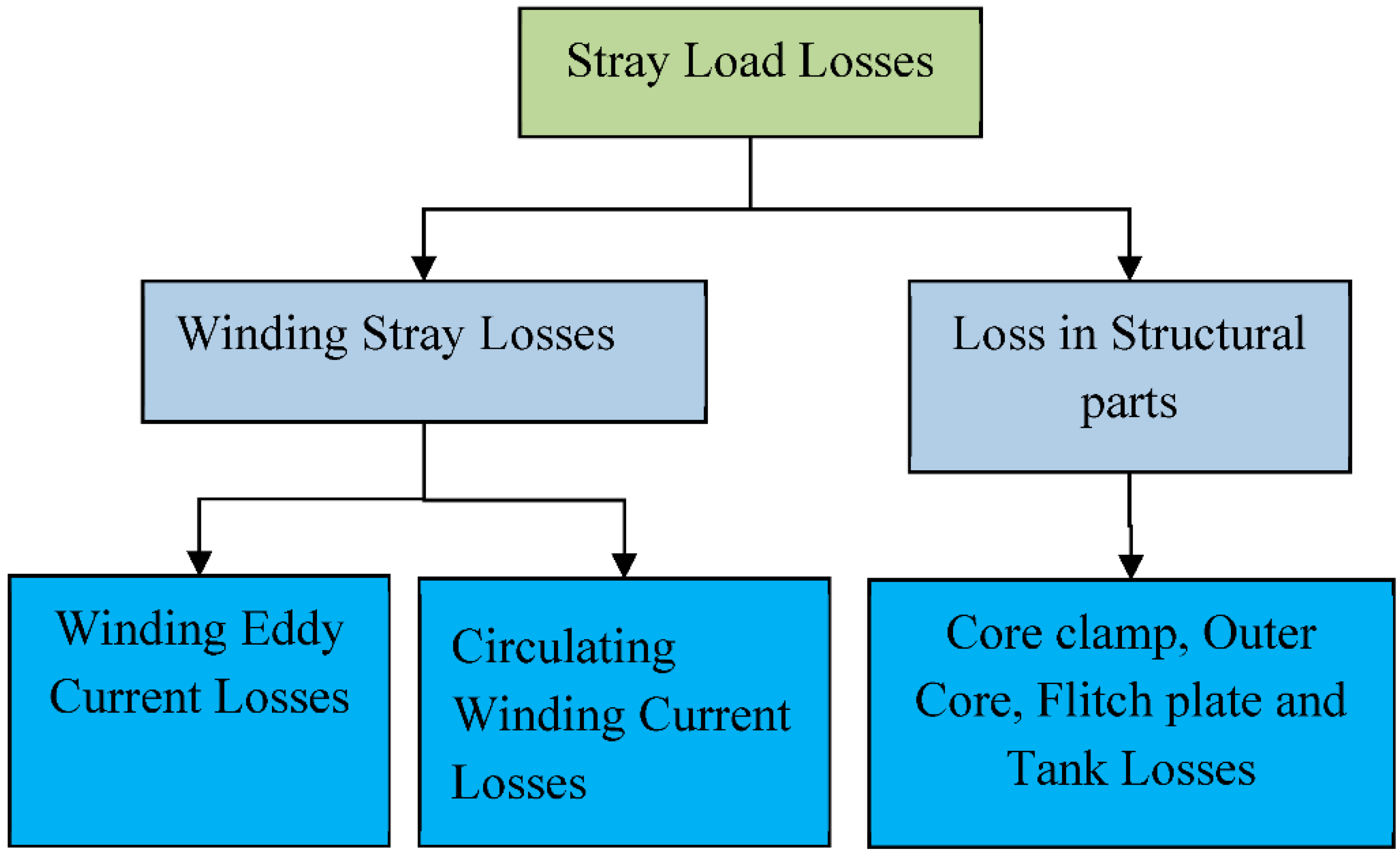
2. Stray Load Loss Components

It can be well established that an electrical transformer is structured as a three dimensional (3D) complex system; therefore, 3D modelling is normally mandatory in order to permit all impelling parameters for optimal solutions. However, 3D FEM simulation requires a cutting-edge simulation program and longer computational time. Common alternatives including part-modelling, the selection of mesh size and 2D modelling may be employed to subdue these drawbacks. By employing 2D modelling, the error of estimate between calculated and measured results can be significantly reduced given that FEM considers parameters that analytical formulations neglect. In the case of a 2D FEM model, the magnetic field parameters in the z-axis are omitted and the main parts of the step-up transformer subject to leakage flux are presented as shown in Figure 5.

The computation of losses in the 2D FEM model is achieved without considerable loss of precision. Accurate computation of the transformer losses is crucial for manufacturers as they are generally stated in the contract by the purchaser (utility owner). Designers are challenged to optimise the transformer design such that minimum losses occur under harmonic load current conditions in the case of renewables and in order to avoid paying penalties. During the design stage, manufacturers rely heavily on the multiple benefits of integrating 2D, 3D and analytical methods to present a comprehensive estimation and optimal transformer losses. The simulation variables are statistically fitted based on field and factory acceptance test (FATs) measurements. The benefits of applying this computational power in the investigation of transformer design parameters that would have not been previously possible are not only restricted to the reduction in cost and computation time but also an in-depth understanding of the literal processes that occur during operation.

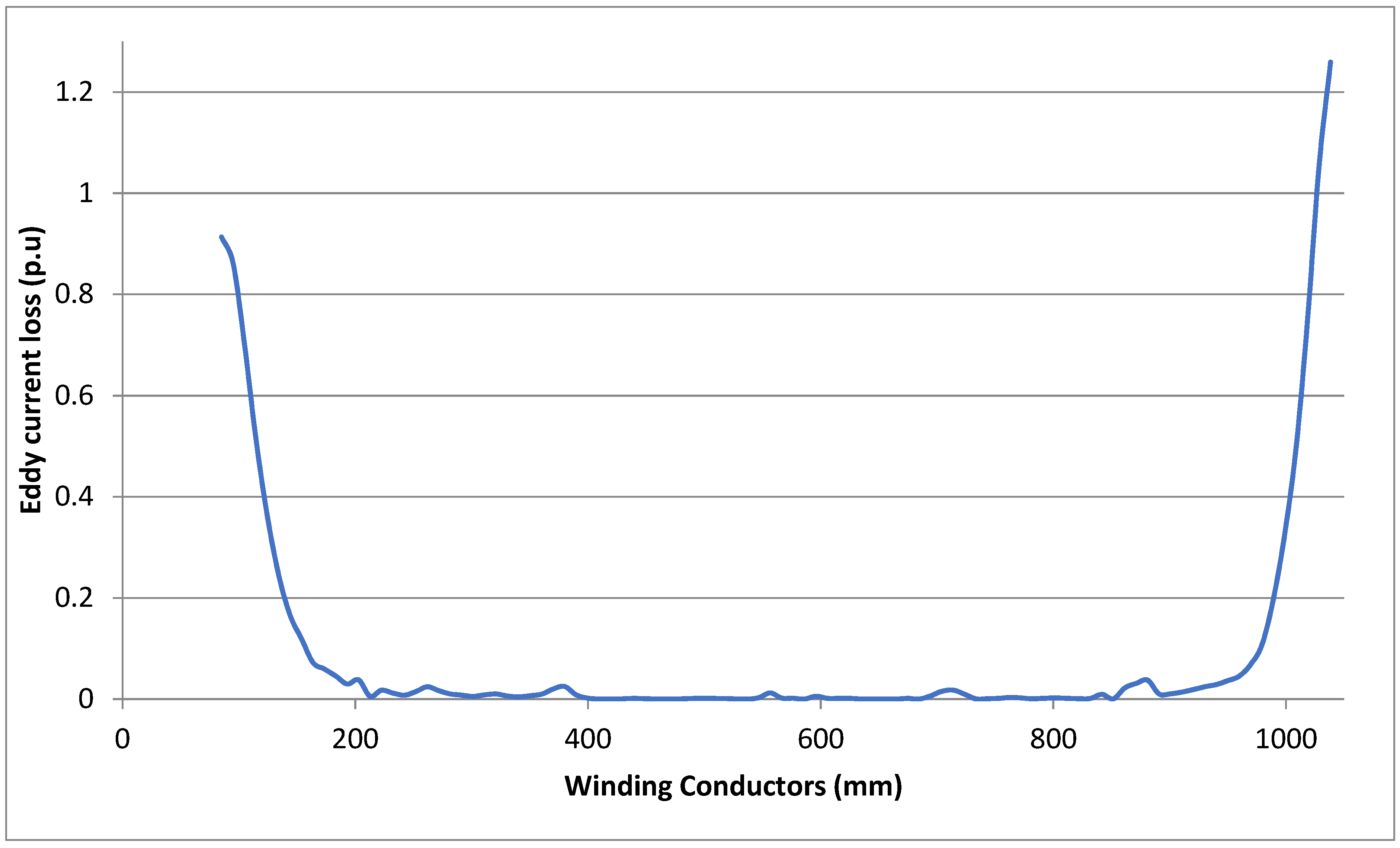
2.1. Winding Eddy Losses

The winding Eddy current losses are a result of the axial and radial stray fields impinging upon the surface of the conductors. Information about the axial and radial flux density segments of the leakage field is crucial for electrical designers to optimally select the axial and radial conductor dimensions.

In 1966, Dowell [22] derived a method for calculating Eddy currents using analytical methods for single-layer, multilayer and sectionalise windings. The method is based on discretising the winding into portions to attain the respective d.c resistances and leakage inductances. Dowell derived factors also presented as curves from theoretical expressions for the variation of frequency and conductor dimensions necessary in obtaining the corresponding a.c parameters. These parameters are then referred to respective windings and summed to give the overall winding resistance and leakage inductance of each winding portion. However, this method suffers from considerable computation due to the iteration required to calculate the d.c leakage inductance and the lack of experimental validation.

In 1967, Stoll [23] described an approach for determining the Eddy currents in transformer winding conductors by utilizing the finite-difference method of successive over-relaxation treated by a digital computer. The method considers the vector potential of Eddy currents in the conductors concerning time and space. Here, the time axis is discretised into a considerable number of time steps and considerable integration computation is required to attain the spatial solution. Stoll reports that relatively large fields must reduce the number of nodes such that the length of the mesh is minimal within the winding conductor and around the Eddy current zone. This is also economical and saves considerable computer memory. Rodger et al. [24] present an approach to model emaciated skin depth Eddy currents in 3D equipment by employing the magnetic potential vector. An analytic solution of the electromagnetic fields in the emaciated skin depth is employed to establish a surface impedance that fulfils the function of a surface integral at the faces of components that synthesize with the emaciated skin Eddy current zone. The approach has been carried out through classical nodal variable finite elements.

On the IEEE standard [25], a technique was formulated to ascertain the efficiency of an in-service transformer to operate under non-sinusoidal load currents, the Eddy current losses are presumed to transform with the square of the root mean square current and the square of the harmonic frequency. This presumption is acceptable for transformers with shorter winding conductors and exposed to low harmonic orders. For large conductors and high harmonics, such an assumption leads to a conservative result. Given the depth of skin effect, the electromagnetic flux might not utterly perforate the copper conductors in the windings at high harmonic orders. Consequently, a power of two deployed in the computation inclines to be conservative [26,27].

Makarov and Emanuel [28] conducted a study to find the corrected harmonic loss factor under harmonic conditions using an analytical approach for conductors with large dimensions. Here, they use the approximation method [29] to ascertain that winding Eddy losses are symmetrical to the square of the hth harmonic order if all their dimensions are less than 3 mm. Cheng [30] presents an approach to determine the winding Eddy losses utilizing the matrix modelling technique. The model attempts to present all winding conductors as small filaments in order of their skin depth. Cheng also uses the model filament in modelling the eddy current distribution within the winding and obtaining the equivalent impedance. The practical results show good accuracy of the model in the frequency region 1 kHz and 1 MHz.

Kulkarni and Khaparde [31] published a book describing a method for Eddy current losses of a square conductor formulated from the Maxwell equations and consider an infinitely long winding conductor in the x-direction along a time-varying magnetic field in the y-direction. The variation of the field quantities viz. current density and intensity of a magnetic field, noting that copper conductors have constant permeability, are simplified to yield a diffusion equation. However, this method ignores the radial magnetic field in the winding end zones. In [32], Bachinger et al. describe a numerical method to treat harmonic eddy currents in conductors using the Multiharmonic solution technique. This method considers the nonlinear correlation between the flux and induction in conductors. The time-dependency of harmonic Eddy currents are taken into consideration by time discretisation using the truncated Fourier series expansion. In this paper, the errors due to the truncated Fourier series expansion, spatial discretisation and regularisation parameters are thoroughly estimated.

A principal indicator of the effects impelled by the harmonic load currents on the winding Eddy losses is the harmonic factor.

A. Elmoudi et al. [33] present a corrected harmonic loss component for winding Eddy losses which consider the depth of penetration. Elmoudi concludes that conservative results lead to higher losses than the factual losses owning to the neglected depth of penetration for conductors with large dimensions at higher harmonic orders. The real magnetic field encroaching on the winding conductors will be slighter as a consequence of the skin effect. A. Van den Bossche et al. [34] reports a practical method for calculating eddy current losses which attempt to improve the classical loss calculation by instituting a loss factor. A graphical approximation of the loss coefficient as a function of wire diameter, frequency, layer number and copper packaging factors are attained by comparing the analytical approach with FEM simulations and substantiated by designing various transformers.

In [35,36], an algorithm to determine Eddy currents in square conductors with source currents employing the integral equation method is formulated. This method considers the finite length of conductors and the cross effect between orthogonal conductors to examine the proximity effect. In the algorithm, the Biot–Savart integral is incorporated to calculate the generated magnetic fields. In comparison with 3D FEM simulations, this algorithm yielded a reduced number of unknowns in the Eddy current calculations upon the winding discs with insignificant error in the 3D topology of the magnetic fields. Larsson [37] also applied the integral equation method to calculate the Eddy currents in conductors. The magnetic fields impinging upon the conductor surfaces are generated by integral relations derived from Green’s function technique. Larsson here incorporates numerical integration to obtain the solution.

The magnetic field solution given by the use of FEM simulation produces a common leakage flux where the flux is axially streaming up along windings through the conductors and then bends radially across the winding end zones. This is a critical point in a transformer as the conductors are susceptible to prone axial and radial flux constituents. Through local magnetic field density encapsulated in transformer design FEM models, the Eddy loss density at hotspot regions can be evaluated.

In a book published by Del Vecchio [38], a geometry for calculating Eddy current losses on account of flux impinging upon the surface of the conductor is presented. The method assumes a square conductor transverse area and the magnetic field vector is disintegrated into elements parallel to the axial and radial dimensions of the conductor. The computation of the losses associated with magnetic fields are performed separately and the results are added. This method is important in such a way as the Eddy currents coupled with respective flux components by no means overlay.

In other recent attempts, Yin and Wei [39] consider Maxwell’s equations and Poynting’s theorem in studying the winding behaviour under harmonics and introduce an AC winding coefficient to establish a winding eddy loss calculation model.

2.2. Winding Circulating Current

The asymmetrical linkage of the leakage field between adjacent strands of the winding with multiple stranded conductors (e.g., helical winding) induces circulating current losses. This loss is highly dependent on the interspace of each strand within the leakage field. During the design stage, the windings are optimised so that the leakage flux is symmetrical within the adjacent strands. The latter is achieved through the continuous transposition of conductors (CTC) at predetermined locations along with the winding height.

Kaul [40] described an analytical procedure to determine circulating current losses in layer and conventional disc windings. Kaul here assumes a voltage slope for the stray current as an arithmetic total of resistive and reactive decrease in electrical potential. The main limitation of this method is that it only considers the axial leakage flux and ignores the radial leakage flux. The results show significant calculation error in large, medium and distribution transformers. Kappikar [41] extended this work by developing a 2D FEM transformer model using MagNet software. Detailed modelling of various winding conductors is carried out as case studies. This approach considers the impact of field response on the main leakage field and radial leakage magnetic field at the winding terminals. However, the drawback of this approach is that it does not independently calculate the circulating current losses but rather as a percentage of the copper losses. Dexin et al. [42] proposed a numerical method to optimise the winding transposition design. The method is based on a multi-section 2D quasiaxi-symmetrical scheme and direct field-circuit coupled method to obtain the actual 3D magnetic fields and to integrate the multi-parameter circuit, respectively. The test result of a 720 MVA double-helical winding indicates that in comparison with physical transpositions the multi-section method yields better results in comparison with the conventional uniform axisymmetric field method.

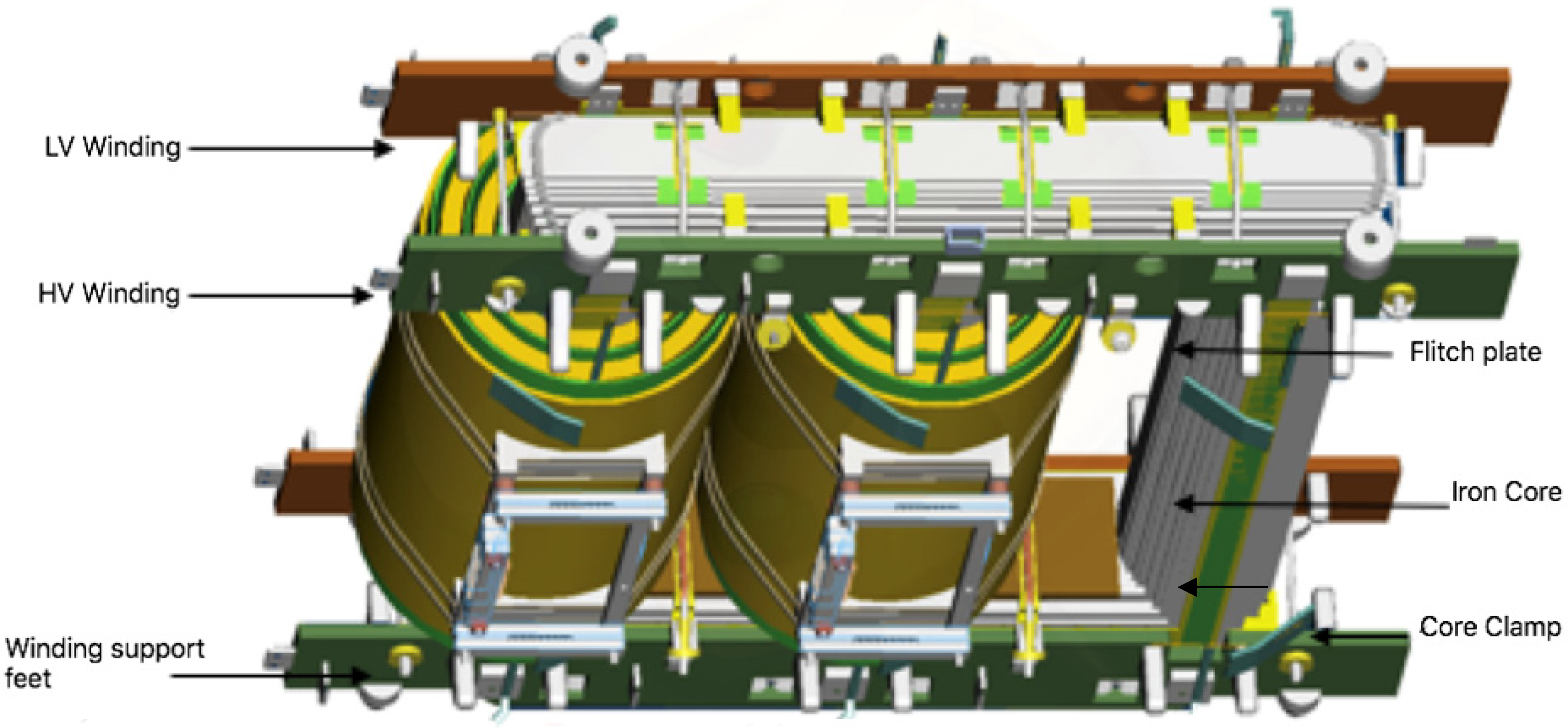
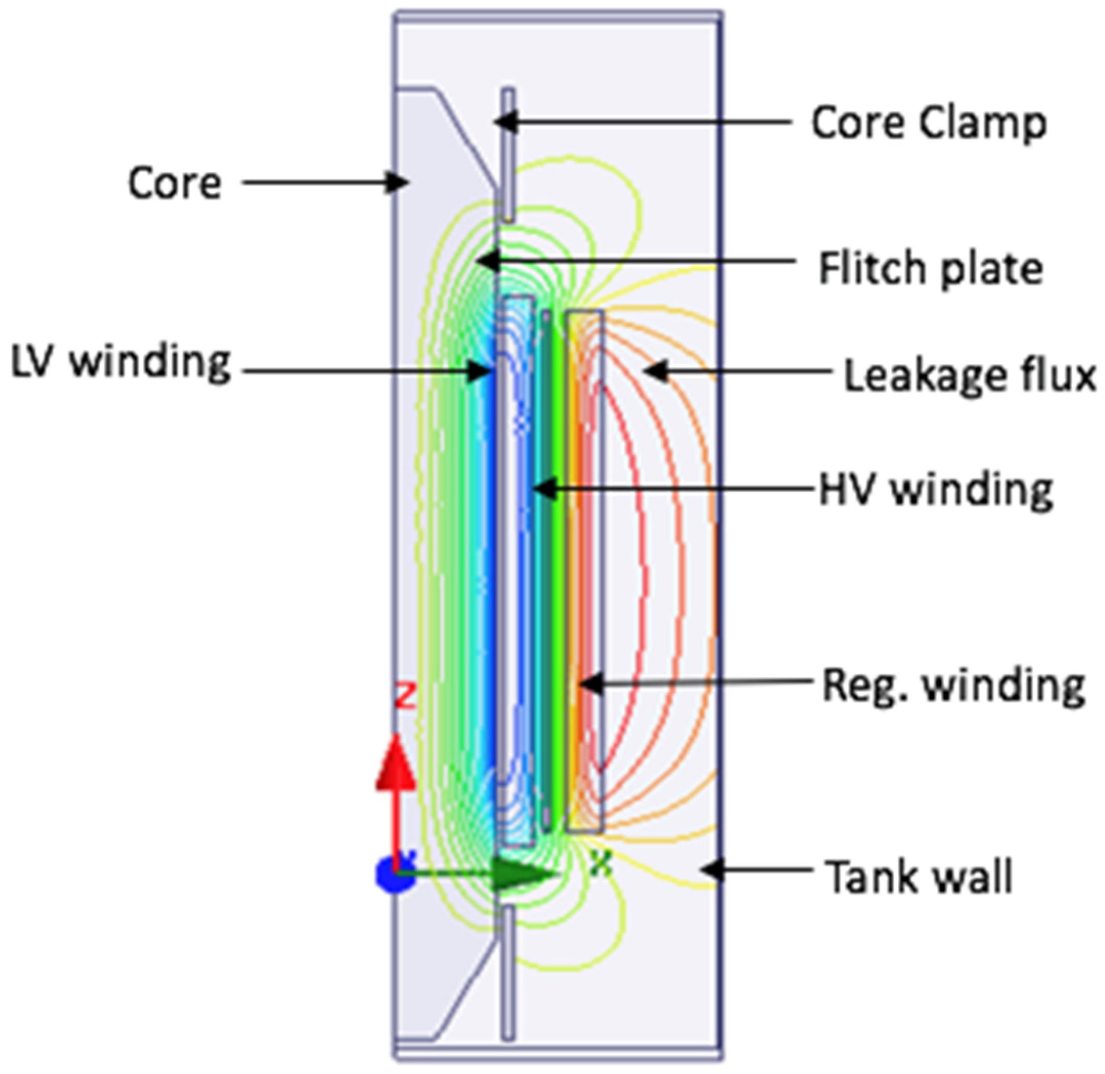
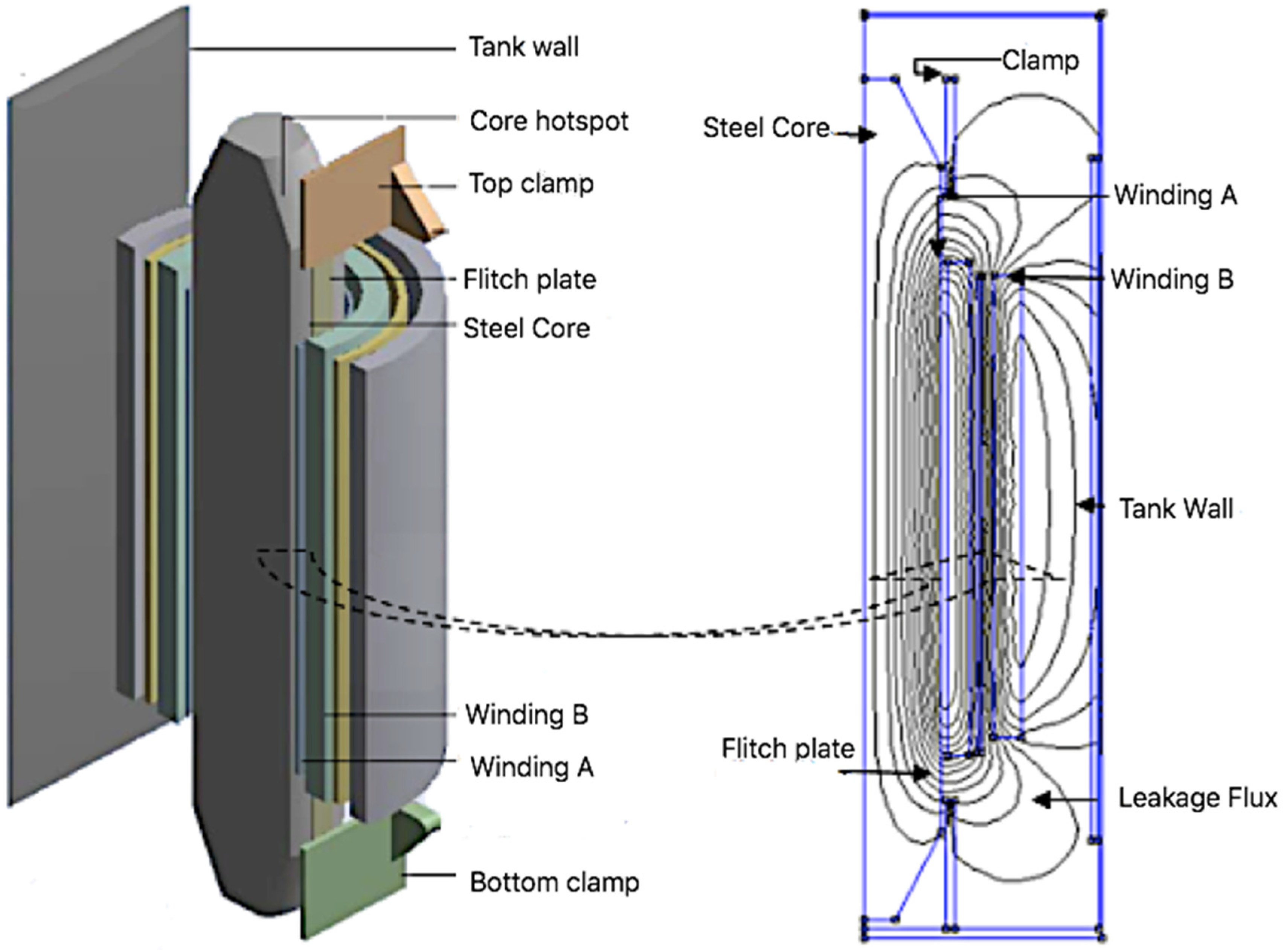
2.3. Stray Loss in Other Structural Parts

Stray load losses in the various transformer active components are primarily results of the main leakage magnetic field culminating radially from the winding surface. Steel tank losses are also on account of the Eddy currents derived from the magnetic fields of the winding leads carrying relatively high current passing nearby and in parallel to the tank walls.

In 1997 [43], Koppikar and Kulkarni et al. described an analytical method to calculate Eddy current losses in the tank walls (mild steel) due to nearby parallel current-carrying conductors. The method considers 2D current distributions including single and three-phase currents and square winding conductors. Stray load loss in tank steel walls is sheltered by an electromagnetic screen is taken into consideration by modifying the analytical formulae. In comparison with the 2D FEM analysis and laboratory experiments, the calculated losses yielded an error of approximately 10%. At large, this paper is still fundamental in developing analytical methods for stray loss calculations in a tank.

Del Vecchio [44] also presented an analytical approach to evaluate the stray loss in tank walls. This method is based on placing current filaments at the corner and centre of each bus bar. In comparison with the variety of rectangular bus bar configurations carrying currents of different magnitudes and phases that were modelled using FEM, the calculated losses produce good results within 1% or 2%. The drawback of this method is that it does not consider the Eddy current redistribution within the bus bars which might lead to a significant error.

Due to the complex nature of the tank geometries, it is of greater interest to use 2D/3D FEM simulations that emerged as early as the 2000s by Kulkarni. In [45], Olivares et al. collaborated with Kulkarni to present a numerical method based on 2D time-harmonic FEM analysis of losses produced in the steel tank walls enclosing high-current bushings. In this publication, the eddy current losses are reduced by inserting a “T” shaped plate near high current phases. The collaboration was also extended for an improved insert geometry in [46] by using 3D time-harmonic FEM solver. The simulation results yielded an error of 7.5% against practical measurements.

In other attempts, Ho et al. [47] formulated a numerical method for a 720 MVA/500 kV to calculate the 3D open boundary eddy current fields impinging upon the tank walls. The method applies the preconditioned complex bi-conjugate gradient method to generate mesh, stiffness matrix and the solution via a source program developed in FORTRAN. After identifying hotspots in the tank walls, Ho et al. find that their choice to select low magnetic permeability steels around the high current carrying bus bars and windings significantly reduced the stray loss in the tank. Ferreira da Luz et al. [48] examined stray loss in a tank due to high current leads using a sub-problem finite element method. The surface impedance technique which reduces computation time is used in modelling the tank geometries.

Measures for stray loss control in the tank can be achieved by mounting magnetic shunts to shield eddy currents on the surface of the tank. The shunts are erected by ferromagnetic laminated steel components that steer the magnetic fields emerging from the bus bars.

Duc et al. [49] described a method to predict stray loss in tank walls by placing shields in the predicted hotspot region. The method optimises the tank shielding using 3D Magneto-thermal coupled simulation. In comparison with the measured values, the simulation results yield a reduction in total stray losses by 11.3% with the highest reduction on the HV tank wall of 52%. Kralj and Miljavec [50] developed a time-harmonic 3D FEM model using a commercial software package Cedrat Flux 3D [51] to compute the magnetic leakage field under nominal load case conditions. The losses are calculated based on the nonlinear surface impedance method which considers the nonlinear magnetic B (H) characteristic of tank material. A more optimised shielding method using magnetic wall shunts modelled with nonlinear high permeability and related stray losses are introduced by Najafi et al. [52] using 3D FEM. The flux shunting properties of this shield allow the electromagnetic flux from the electromagnetic source to be directly drawn into the magnetic material. Wiak et al. [53] present a methodology to eliminate Eddy losses in the tank by introducing an approach of effective tank screening by magnetic screen covers using 3D FEM calculations. The tank losses are computed as being integral to the current density and field strength for each subdomain. Magnetic shielding of the tank was also employed by Li et al. [54]. where the stray losses and Eddy current field are calculated using the MagNet software. The results indicate that a maximum stray loss and loss density of the core clamp is reduced by 48.9% and 43.1%, respectively. Li et al. [55] also employed the 3D MagNet software to calculate the stray losses in tank walls and yoke clamps by considering the nonlinear magnetic B (H) characteristic of tank material. The analysis of the electromagnetic fields in the model is based on the T-Ω method which represents the magnetic field as the sum of scalar potential gradient, and in the winding conductors, an additional vector field represented by Whitney edge elements.

In other attempts, Krasl et al. [56] present a 3D FEM approach to calculate losses in a transformer tank and frame produced by a stray magnetic field from the windings. Due to the large surface area-efficient cooling seldom develops and the frame losses are calculated using the Finite Difference Method (FDM). Another but less accurate method that makes use of the 3D Reluctance Network Method is mentioned. Krasl et al. propose a reduction in losses by using laminated and resistivity material, reduction in flux density in the component by diverting the incident flux by the use of a shielding plate and the use of material with lower permeability. Yan et al. [57] present a method with less computational time that integrates 3D FEM and analytical techniques for calculating the stray losses. The magnetic flux and Eddy current density impinged on the surface of the metallic part are obtained by FEM and then utilised to calculate stray losses using the analytical approach.

An improved method with less computational effort is also described by Yan et al. [58] using double Fourier series to represent the magnetic flux density. The least mean error accompanied by a curve fitting technique and an optimisation algorithm is used to compute the coefficients of the Fourier series. The resultant eddy losses are attained by analytical formulae based on the theory of Maxwell equations. A similar study based on the double Fourier series expansions was carried out by Moghaddami et al. [59] on a 200 MVA power transformer using 3D FEM in COMSOL Multiphysics. A Parametric FEA is carried out to find the optimised position to place the horizontal shunts on the tank walls. Stray load losses on the tank walls and yoke beams are calculated using a surface impedance boundary condition.

Losses in the core fittings such as flitch plates and core edges are due to the leakage flux emerging from the inner surface of the windings.

3. Theoretical Foundation of Eddy Currents

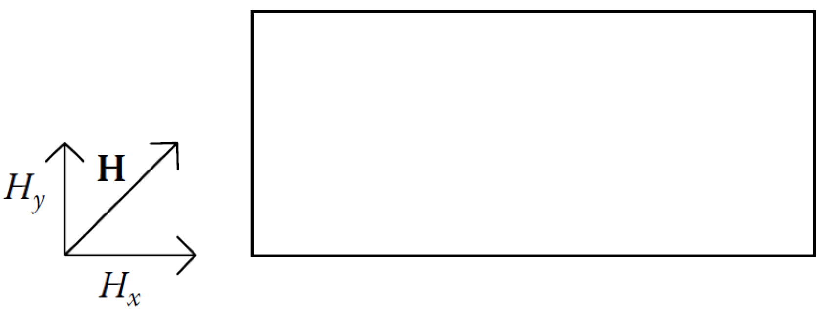
3.1. Generation of Electromagnetic Fields in Conductors

In core-type transformers, the HV and LV windings are cylinders with a common centre encircling vertical magnetic core limbs with circular cross-sections [60]. The vertical magnetic core limbs and the horizontal core yoke components are made of thin laminated sheets and provide a magnetic flux circuit. On the top and bottom core yokes, there are core clamping structures that stabilise the LV and HV windings assembly on the magnetic steel core. The active part components of oil-immersed transformers are enclosed with rectangular steel tank walls as illustrated in Figure 6. If load current flows within the winding copper conductors, a loss (I2R) will be generated. The individual current-carrying conductors are encompassed by alternating electromagnetic fields with an intensity proportional to the load current [60]. The field composition generated by the load current is illustrated in Figure 6, which is a two-dimensional model of the transformer active part components as indicated [60]. Individual winding conductors encompassed by alternating electromagnetic fields encounter an internally induced voltage that triggers the generation of the winding Eddy currents to flow in respective winding conductors [60]. These currents bring out losses in the conductors and are dissipated inherently as heat, generating a rise in temperature in the conductors and surrounding metallic structures. The additional losses outside the copper loss are by and large described as the stray losses. Even though the additional losses are Eddy current losses, only the fraction in the windings is described as the “winding Eddy loss”, and the remaining loss component is contributed by the metallic active parts and can be described as the “other stray losses” [60].

The winding Eddy losses are directly proportional to the load current that produces the electromagnetic fields and the square of the fundamental frequency (50 Hz) [60]. The other stray losses by the transformer manufacturer’s in-house statistical surveys are largely proportional to the load current to an exponent slightly less than 1, considering that the depth of penetration by the fields into the other metallic structures is proportional to the field intensity [60]. In the event of high harmonic load currents, the magnetic flux may not wholly permeate the surface of the winding conductors whatsoever, a conventional approach is to conservatively presume that the winding Eddy losses are proportional to the harmonic order. When the unit in-service is exposed to considerable harmonic load current components, the additional winding Eddy losses and other stray losses will yield a rise in temperature beyond admissible temperature at rated conditions [60].

Experience has indicated that the transformer winding conductors are the most critical active components in evaluating the admissible operational temperature of the transformer. Consequently, the manufacturers are challenged with obviating the winding losses under harmonic conditions from surpassing the losses of the unit operating at a fundamental frequency.

The LV winding generally has a higher winding Eddy loss in comparison with the HV winding, owing to the fact that the magnetic flux has an increasing tendency to ruffle in the direction of the lesser reluctance pathway of the core limbs [60]. In addition, the greatest local Eddy loss normally materialises towards the nearer end winding conductors of the LV winding in view of the fact that the area of concentrated magnetic flux radial lines (Figure 6) passes through the radial direction of the individual winding conductor dimensions. The inherent nature of the winding Eddy current loss distribution computed by the authors is shown in Figure 7.

Considering that in practice the conductor width is approximately 3.1 to 5.5 times the conductor thickness and the winding Eddy loss is proportional to the winding conductor dimensions, significant loss rises in the near-end conductors of the winding.

3.2. Eddy Current Loss Formulation in Time-Varying Fields

To analyse the impact of leakage flux in the winding losses, a single rectangular conductor that may be a member of a Continuously Transposed Cable (CTC), which is composed of several rectangular [60], PVF (polyvinyl formal) enamelled copper conductors assembled into a bundle may be studied. The magnetic flux at the location of the winding conductor will point in a particular direction with respect to the conductor’s position. This vector can be disintegrated into axial and radial parts parallel to each face of the conductor as illustrated in Figure 8 [60].

The loss related to an individual component of the magnetic flux must be evaluated independently and sum the results of the individual components. This may provide some accuracy such that the Eddy currents related to the respective field components do not intersect [60]. In order to derive the winding Eddy losses, we may consider the radial losses intricately connected to the y-component of the external field as illustrated in the coordinate system in Figure 9 [60]. We assume the length of the winding conductor is in the Z-direction. In this regard, the fields are independent of the no z-component and an assumption is made that they only have the y-component.

By applying Maxwell’s Equation (1) in the reference coordinate system above and the aforementioned assumptions, the following differential form equations for time-dependent magnetic fields in the location of the conductors will apply [60]:

$$\begin{array}{c}\nabla \times \mathit{E}=-\frac{\partial \mathit{B}}{\partial t}\gg \frac{\partial {\mathit{E}}_{\mathit{z}}}{\partial x}=\mu \frac{\partial {\mathit{H}}_{\mathit{y}}}{\partial t}\\ \nabla \times \mathit{H}=\mathit{J}\gg \frac{\partial {\mathit{H}}_{\mathit{y}}}{\partial x}={\mathit{J}}_{\mathit{z}}\\ \nabla \times \mathit{B}=\mathbf{0}\gg \frac{\partial {\mathit{H}}_{\mathit{y}}}{\partial y}=\mathbf{0}\end{array}$$

(1)

where

• $\mathit{E}—$Electric field strength ($\mathrm{V}/\mathrm{m}$)
• $\mathit{B}—$Flux density ($\mathrm{wb}/{\mathrm{m}}^2$)
• $\mu —$Permeability of material ($\mathrm{H}/\mathrm{m}$)
• $\mathit{H}—$Magnetic field strength ($\mathrm{A}/\mathrm{m}$)
• $\mathit{J}—$Current density ($\mathrm{A}/{\mathrm{m}}^2$)

In the winding conductor, Ohm’s law can be expressed in the form as follows in Equation (2) [60].

$$\mathit{J}=\sigma \mathit{E}\gg {\mathit{J}}_{\mathit{z}}=\sigma {\mathit{E}}_{\mathit{z}}$$

(2)

where

• $\sigma —$conductivity ($\mathsf{\Omega }\cdot \mathrm{m}$)

As illustrated in Equation (2), the current density and electric field strength are only dependent on the z-component along the length of the conductor as highlighted on the reference coordinate system for loss computation. Now, combining Equations (1) and (2), the results yield Equation (3) [60].

$$\frac{{\partial }^2{\mathit{H}}_{\mathit{y}}}{\partial x^2}=\mu \sigma \frac{\partial {\mathit{H}}_{\mathit{y}}}{\partial t}$$

(3)

Here, ${\mathit{H}}_{\mathit{y}}$ is a function of the variables $x$ and $t$ with a sinusoidal form as follows in Equation (4) [60].

$${\mathit{H}}_{\mathit{y}}\left(x,t\right)={\mathit{H}}_{\mathit{y}}\left(x\right)e^{j\omega t}$$

(4)

It follows that Equation (4), can then be expressed as shown in Equation (5) [60].

$$\frac{{\partial }^2{\mathit{H}}_{\mathit{y}}}{\partial x^2}=j\omega \mu \sigma {\mathit{H}}_{\mathit{y}}=k^2{\mathit{H}}_{\mathit{y}}$$

(5)

Using Equation (5), along the axial direction of the conductor, ${\mathit{H}}_{\mathit{y}}$ is solely a function of the independent variable $x$ and yields the solution in Equation (6) when solved with the boundary conditions $x=\pm b/2$ in the horizontal direction of the conductor shown in Figure 9 and ${\mathit{H}}_{\mathit{y}}={\mathit{H}}_{\mathbf{0}}$ [60].

$${\mathit{H}}_{\mathit{y}}\left(x\right)={\mathit{H}}_{\mathbf{0}}\frac{\cos \mathrm{h}\left(kx\right)}{\cos \mathrm{h}\left(kb/2\right)}$$

(6)

Here, ${\mathit{H}}_{\mathbf{0}}$ is the amplitude of the magnetic field strength and $b$ is the width of the winding conductor shown in Figure 9. Applying Equation (1), the current density along the length of the winding conductor can be expressed as follows in Equation (7) [60].

$${\mathit{J}}_{\mathit{z}}=-k{\mathit{H}}_{\mathbf{0}}\frac{\sin \mathrm{h}\left(kx\right)}{\cos \mathrm{h}\left(kb/2\right)}$$

(7)

The Eddy current loss per volume along the length of the winding conductor can then be expressed as follows in Equation (8) [60].

$$P_{EC/unitlength}=\frac{c}{2\sigma }{{\displaystyle \int }}_{-b/2}^{b/2}{\left|{\mathit{J}}_{\mathit{z}}\right|}^{2}dx=\frac{c{\mathit{H}}_{\mathbf{0}}{\left|k\right|}^2}{\sigma {\left|\cos \mathrm{h}\left(kb/2\right)\right|}^2}{{\displaystyle \int }}_0^{b/2}{\left|\sin \mathrm{h}\left(kx\right)\right|}^{2}dx$$

(8)

Here, $c$ is the height of the winding conductor along the direction of the field as shown in Figure 9. The coefficient ½ is derived from obtaining the meantime and applying maximum values of the field. Applying integration halfway the thickness on the winding conductor with the limits $x=\pm b/2$ due to symmetry of the integrated function, the coefficient is cancelled. The latter yields Equation (9) [60].

$$k=\left(1+j\right)\sqrt{\frac{\omega \mu \sigma }{2}}=\left(1+j\right)q;\mathrm{where},q=\sqrt{\frac{\omega \mu \sigma }{2}}$$

(9)

By applying this expression, the hyperbolic functions in Equations (10) and (11) are obtained [11].

$${\left|\sin \mathrm{h}\left(kx\right)\right|}^2=\frac{1}{2}\left[\cos \mathrm{h}\left(2qx\right)-\cos \left(2qx\right)\right]$$

(10)

$${\left|\cos \mathrm{h}\left(kx\right)\right|}^2=\frac{1}{2}\left[\cos \mathrm{h}\left(2qx\right)+\cos \left(2qx\right)\right]$$

(11)

Substituting these hyperbolic functions into Equation (8), finding the integral solution, and dividing by the cross-sectional area of the winding conductor, the particular winding Eddy loss (in $\mathrm{watts}/{\mathrm{m}}^3$) can be expressed as follows in Equation (12) [60].

$$P_{EC}=\frac{{\mathit{H}}_{\mathbf{0}}{}^{2}q}{\sigma b}\left[\frac{\sin \mathrm{h}\left(qb\right)-\sin \left(qb\right)}{\cos \mathrm{h}\left(qb\right)+\cos \left(qb\right)}\right]$$

(12)

At low frequency, the value of $qb$ approached infinity and the equation is reduced as follows in Equation (13) [60].

$$P_{EC}\to \frac{{\mathit{H}}_{\mathbf{0}}{}^2{q}^4{b}^2}{6\sigma }=\left(\frac{{\pi }^2}{6}\right)f^2{\mu }^2{b}^2\sigma {\mathit{H}}_{\mathbf{0}}{}^2=\left(\frac{{\pi }^2}{6}\right)\frac{f^2{b}^2{B}_0{}^2}{\rho }$$

(13)

where

• $\rho —$resistivity of a conductor ($\mathsf{\Omega }\cdot \mathrm{m}$).

4. Electric Transformer Losses

The total transformer losses are holistically catalogued as a total of the no-load losses, copper losses, winding Eddy losses and other stray losses as follows in Equation (14). The no-load losses materialise when the transformer is energised in conformity with the nameplate ratings. However, the low voltage (LV) winding is open circuited in a way that the no-load current is flowing through the winding conductors. The no-load losses arise from harmonic voltage excitation of the core steel material [61,62].

$$P_{TOT}=P_{NLL}+P_{LL}=P_{cu}+P_{WEC}+P_{OSL}$$

(14)

where

• $P_{LL}—$Load loss (in kW)
• $P_{NLL}—$No-load loss (in kW)
• $P_{cu}—$Copper loss (in kW)
• $P_{WEC}—$Winding Eddy loss (in kW)
• $P_{OSL}—$Other Stray loss (in kW)

The load losses can be fragmented into the copper loss and stray losses (the total of $P_{WEC}$ and $P_{OSL}$) and are triggered by the time-varying magnetic flux in the tank walls, core clamping structures, flitch plates, core steel, winding conductors, et cetera. The copper losses can be evaluated from the measured winding resistance. The stray losses can be ascertained by subtracting the copper losses from the load losses. The measurement of the stray losses is not practically feasible. In practice, the percentage distribution of the losses in various metallic structures can then be computed by FEM simulations. This thesis also aims to contribute some insights into the stray loss distribution, particularly for solar PV transformers in the South African grid.

4.1. Copper Loss under Harmonic Conditions

The copper loss can be estimated by multiplying the square of the root mean square (r.m.s) load current and the measured resistance. Under harmonic load current, the copper loss can be expressed as follows in Equation (15) [62].

$$P_{cu}=P_{cu\left(Rated\right)}\times \sqrt{{\displaystyle \sum }_{h=1}^{h=max}{I}_h{}^2}$$

(15)

here,

• $P_{cu}—$Copper loss under harmonic conditions
• $P_{cu\left(Rated\right)}—$Copper loss at rated conditions
• $h—$Harmonic order
• $I_h—$Harmonic load current

If the effective r.m.s per-unit harmonic load current evaluated according to the supplied harmonic spectrum increases, then the copper losses will also be increased appropriately.

4.2. Winding Eddy Loss under Harmonic Conditions

The winding Eddy load loss under distorted harmonic currents inclines with the square of the harmonic load current and has a constant relation with the harmonic order as in Equation (16).

$$P_{WEC}=P_{WEC\left(Rated\right)}\times F_{H{L}_{WEL}}$$

(16)

It is appropriate to describe a single value to that may which could be applied to evaluate the transformer capability when delivering power to the connected load. It is this feature that accounts for the inflated winding Eddy losses and subsequently temperature rise and generation of hotspots in the winding conductors. From the above, it can be additionally seen that the proportionality factor $F_{H{L}_{WEL}}$ is the ratio of the winding Eddy loss under harmonic conditions and at a fundamental frequency, respectively. The description of the factor is expressed as follows in Equation (17) [61,62].

$$F_{H{L}_{WEL}}={\displaystyle \sum }_{h=1}^{h=max}{h}^2{\left[\frac{I_h}{I_R}\right]}^2/{\displaystyle \sum }_{h=1}^{h=max}{\left[\frac{I_h}{I_R}\right]}^2$$

(17)

Equation (17) allows the harmonic factor to be computed in response to the effective r.m.s value of the distorted harmonic currents. Harmonic analysers including Tektronix, Rohde and Fluke allow computations to be carried out in response to the harmonics standardized to the fundamental harmonic.

4.3. Other Stray Loss under Harmonic Conditions

The stray load losses are formed by the stray magnetic fields encroaching above the covering of various active parts. When a unit in-service is susceptible to harmonic currents, these losses will tend to also increase. These losses under harmonic load conditions can be evaluated as follows in Equation (18).

$$P_{OSL}=P_{OSL\left(Rated\right)}\times F_{H{L}_{OSL}}$$

(18)

The stray load losses in the steel tank walls, silicon steel core clamping structures, flitch plates, core steel, winding copper conductors et cetera also are inclined to increase with the harmonic load current. At the same time, these losses will augment at a value proportional to the exponent 0.8 of the distorted harmonic order. The effective r.m.s heating resulting from these losses triggers overheating of the insulating oil. This effect may be evaluated by the other stray loss harmonic factor as expressed in Equation (19) [61,62].

$$F_{H{L}_{OSL}}={\displaystyle \sum }_{h=1}^{h=max}{h}^{0.8}{\left[\frac{I_h}{I_R}\right]}^2/{\displaystyle \sum }_{h=1}^{h=max}{\left[\frac{I_h}{I_R}\right]}^2$$

(19)

The exponent of 0.8 has been substantiated by empirical studies carried out by manufacturers based on their in-house best practice and is a mainstream practice in the industry.

4.4. Transformer Maximum Loading Capacity

A method for evaluating the admissible operating conditions of new and in-service transformers may be based on the computation of the transformer capacity by deriving a maximum current de-rating factor when supplying a harmonic load current. The winding loss that will be generated on account of supplying a harmonic load current at a region of high winding Eddy loss is calculated as follows in Equation (20).

$$P_{LL}=I^2{}_{\left(pu\right)}\times \left(1+F_{WEC}\times P_{EC\_R\left(p·u\right)}\right)$$

(20)

In Equation (21), the calculation of the maximum per-unit r.m.s current under a harmonic load current is then provided. The latter will facilitate the guarantee that the concentrated locale of losses in the winding conductors does not surpass the losses at fundamental frequency conditions.

$$I_{max}\left(pu\right)=\sqrt{\frac{P_{LL-R}\left(p·u\right)}{1+F_{WEC}\times P_{WEC-R}\left(p·u\right)}}$$

(21)

The product of the rated current and the result of Equation (21) will then yield the maximum rated current in Amps.

4.5. Winding Eddy Loss Corrective Functions

It is iterated that at high harmonic orders, the magnetic flux may not wholly permeate the winding conductors. In Section 4.2, the IEEE standard [15] makes the presumption that the winding Eddy loss is commensurate with the square of the harmonic load current and the harmonic order. In consideration of the skin effect condensed in the vicinity of the surface of the winding conductors at high harmonic orders as demonstrated in Figure 10, the aforementioned presumption does not hold.

When the harmonic load current flows through the winding conductors, Eddy currents are produced in a pattern tending to impede the situation of the magnetic field within the winding conductors. The dispersion of the current over the conductor’s cross-sectional area and the effective resistance between two conductors are on that account functions of load current frequency. When the harmonic load frequency increases, the harmonic load current tends to be centralised on the conductor surface. This calls for a need to derive a method to accurately estimate the winding Eddy losses under harmonic load currents.

4.6. Emanuel et al. Winding Eddy Loss Correction Function

A correction function for estimating the winding Eddy losses under harmonic conditions was proposed by Emanuel et al. in [63]. Their correction function is based on the expression in Equation (22).

$$\Delta P_{EC}={\left(\frac{n\pi fh{\widehat{B}}_x}{\sqrt{6}}\right)}^2\left(1+{\delta }_{bh}{}^2{\beta }_{xy}{}^2\right)\gamma F_H$$

(22)

where

• $nf—$Frequency of the sinusoidal magnetic field
• $\gamma —$Specific conductor conductivity
• $b,h—$Width and height of the conductor
• ${\widehat{B}}_x,{\widehat{B}}_y—$Local induction axial and radial components
• ${\delta }_{bh}—b/h$ Ratio of width and height of the conductor
• $F_H—$Winding Eddy loss correction function

The corresponding correction function is based on the expression in Equation (23).

$$F_H=\frac{6}{{\beth }^3}\times \frac{\sin \mathrm{h}\beth -\sin \beth }{\cos \mathrm{h}\beth +-\cos \beth }$$

(23)

The conductor dimension in relation to the depth of skin effect can be expressed as follows in Equation (24).

$$\beth =h\sqrt{\pi {\mu }_0\gamma nf}$$

(24)

4.7. Thango et al. Winding Eddy Loss Correction Function

The presumption that the winding Eddy loss is proportional to the square of the harmonic load current and the harmonic order is only realistic for winding conductors with small dimensions. In the case of larger conductor dimensions, the aforementioned presumptions culminate in a conservative estimation of the winding Eddy loss. In this thesis, a winding Eddy loss correction function that results in increased accuracy in the projection of the transformer capability under harmonic load currents is formulated. The corrected function proposed in this thesis is published by the author in the article [60] as one of the contributions of this thesis is as follows in Equation (25).

$$P_{EC}=\left(\frac{{\pi }^2}{6}\right)\frac{f^2{b}^2{B}_0{}^2}{\rho }$$

(25)

The Eddy current perplexity appertain to the area of quasi-stationary electromagnetic impacts of conductors, such that the displacement current confined by winding conductors may continuously be neglected with respect to the conducting current. This is assuredly the case even at high harmonic orders, considering in practice only winding conductors including high electroconductivity are utilized. Eddy currents contribute to the irregular distribution of current density in an investigated transversal section of a conductor. This intrinsically ignites to rise in joule heating in contrary to the state generated by direct current (DC). The Eddy currents and associated irregular distribution of the magnetic fields are recognized as the skin effect. The surge in current density brings about Joule heating in preference to the DC resistance in addition to a diminution in the inductance. In resolving the skin effect perplexity, this work espouses and the Maxwell equations are remodelled to solve the quasi-stationary electromagnetic effects of conductors [60].

Here, the proposed correction function is derived as follows in Equation (26). The formulation of this correction function is detailed in [60].

$$F_H=\frac{3}{\beth }\times \frac{\sin \mathrm{h}\beth -\sin \beth }{\cos \mathrm{h}\beth -\cos \beth }$$

(26)

where

• $\beth —$Conductor skin depth in relation to the conductor thickness

It follows that the conductor skin depth in relation to the conductor thickness can be expressed as follows in Equation (27).

$$\beth =\frac{H_{conductor}}{\delta }$$

(27)

where

• $H_{conductor}—$Conductor thickness
• $\delta —$Winding conductor skin depth

At the fundamental frequency (50 Hz) the conductor skin depth in relation to the conductor thickness is expressed as follows in Equation (28).

$${\delta }_R=\sqrt{\frac{\rho }{\mu \pi f}}$$

(28)

Under harmonic load currents, the conductor skin depth in relation to the conductor thickness is expressed as follows in Equation (29).

$$\delta =\sqrt{\frac{\rho }{\mu \pi hf}}=\frac{{\delta }_R}{\sqrt{h}}$$

(29)

The correction function is demonstrated in Figure 11. It can be observed that for small values of the conductor skin depth in relation to the conductor thickness, the correction function yields approximately 1.

By applying Equation (29), the conductor skin depth of a rectangular copper conductor at a fundamental frequency of 50 Hz and 75 °C is 10.63 mm.

Under harmonic load currents, the proportionate skin depth in respect of the rectangular conductor dimensions can be expressed as follows in Equation (30):

$${\beth }_h=\frac{H_{conductor}}{\raisebox{1ex}{${\delta }_R$}\!\left/ \!\raisebox{-1ex}{$\sqrt{h}$}\right.}={\beth }_R\sqrt{h}$$

(30)

The additional winding Eddy losses that will be yielded under the proposed correction function which considers the skin depth at high harmonic order is expressed as follows in Equation (31):

$$P_{WEC}=P_{WEC\left(Rated\right)}\times {\displaystyle \sum }_{h=1}^{h=max}{F}_H{h}^2{\left[\frac{I_h}{I_R}\right]}^2$$

(31)

Standardising the winding Eddy loss generated by harmonic load current to the winding Eddy loss under a rated condition leads to a correction harmonic loss factor is expressed as follows in Equation (32).

$$F_{H{L}_{WEL}}={\displaystyle \sum }_{h=1}^{h=max}{F}_H{h}^2{\left[\frac{I_h}{I_R}\right]}^2/{\displaystyle \sum }_{h=1}^{h=max}{\left[\frac{I_h}{I_R}\right]}^2$$

(32)

The significance of the loss factor above is illustrated in Figure 12, where the harmonic loss function is plotted concerning the harmonic order for a winding conductor with a thickness of 6.4 mm at 75 °C.

It may be observed that the skin effect emerges to have an impact at the fourth harmonic order. For small winding conductor dimensions, the skin effect is only significant at high harmonic orders. The IEEE method is observed to approach $h^2$ as the harmonic order increases as a result of the neglected depth of penetration. The proposed loss factor considers both the effect of the axial and radial conductor dimensions and the field impinging upon the surface of the conductor is observed to be less as a result of the skin effect.

5. Conclusions

In the modern-day South African energy mixed market, unerring evaluation and consequently optimization of electric transformer stray load loss by avant-garde techniques such as FEM will furnish one-upmanship among competing transformer manufacturers. This article has examined all the components that make up the stray load loss in electrical transformers from a perspective of assessment approach, control and alleviation of hotspot regions. In the interest of calculation and controlling stray load loss components in the winding conductors, namely, the winding Eddy current loss and circulation current loss, 2D methods, analytical and numerical methods have been triumphantly employed. Endeavours compelled for 3D analysis may be well-founded, particularly for large power rating electric transformers where the amelioration in precision will be considerable.

Rigorous analysis of loss of flitch plates can be performed by 3D FEM since analytical formulations are erroneous on account of numerous approximations.

Tank loss evaluation constitutes a 3D problem and predominantly transformer manufacturers have adopted the use of 3D FEM to accurately evaluate and manage this loss. Loss in Frames can be computed with reasonable accuracy by using 2D FEM.

Transformers that are intended to operate in harmonically contaminated environments, the adoption of correction factors detailed in this work will aid in alleviating the Eddy current losses and, subsequently, the hotspot regions. This information is critical when designing a cooling system adequate for the losses that will occur.

Transformers designed for renewable sources known to have harmonics, such as wind and solar, will benefit from the methodology discussed herein. These renewables have proven to have total life cycle gas emissions that are much lower than that of conventional coal, particularly in South Africa, with an average of 34.3 and 50.1 g of carbon dioxide per kilowatt-hour.

In hindsight, this article divulges that a prudent choice of method for evaluating the various stray load loss components has to be determined by the electrical transformer designer, wherefore adequate knowledge is furnished in this article.

References

1. GreenCape. Utility-Scale Renewable Energy-Market Intelligence Report; GreenCape: Cape Town, South Africa, 2019. [Google Scholar]
2. The World Bank. Solar Resource Data: Solargis; The World Bank: Washington, WA, USA, 2017. [Google Scholar]
3. SolarPower Europe. Global Market Outlook; SolarPower Europe: Brussels, Europe, 2018–2022. [Google Scholar]
4. Utility-Scale Photovoltaic Procedures and Interconnection Requirements. Available online: https://digital.library.unt.edu/ark:/67531/metadc828656/m2/1/high_res_d/1051725.pdf (accessed on 27 January 2022).
5. Mantosh, D. Investigation of High-Frequency Switching Transients on Wind Turbine Step-Up Transformers. Master’s Thesis, University of Waterloo, Waterloo, ON, Canada, 2015. [Google Scholar]
6. Gurleyen, H. Analysis of Magnetic Coupling Between Armature and Field Windings of VFRM. In Proceedings of the 2021 IEEE International Magnetic Conference (INTERMAG), Lyon, France, 26–30 April 2021; pp. 1–5. [Google Scholar] [CrossRef]
7. Khanali, M. Effects of Distorted Voltages on the Performance of Renewable Energy Plant Transformers; Semantic Scholar: Waterloo, ON, Canada, 2017. [Google Scholar]
8. Liang, S.; Hu, Q.; Lee, W. A survey of harmonic emissions of a commercial operated wind farm. In Proceedings of the IEEE Industrial and Commercial Power Systems Technical Conference, Tallahassee, FL, USA, 9–13 May 2010. [Google Scholar]
9. Tentzerakis, S.; Papathanassiou, S.; Papadopoulos, P.; Foussekis, D.; Vionis, P. Evaluation of wind farm harmonic current emissions. In Proceedings of the European Wind Energy Conference (EWEC), Milan, Italy, 7–10 May 2007. [Google Scholar]
10. Overett, J.S. Assessment of the Harmonic Behavior of a Utility-Scale Photovoltaic Plant. Ph.D. Thesis, Stellenbosch University, Stellenbosch, South Africa, 2017. [Google Scholar]
11. Sokolov, V.V. Transformer is Gassing—What to Do; Scientific and Engineering Center ZTZ-Service Company: Zaporozhye, Ukraine, 2013. [Google Scholar]
12. Zhao, C.; Huang, Q.; Li, D.; Bai, H.; Cheng, Y. The statistical distribution of the DGA data of transformers and its application. In Proceedings of the 2016 IEEE International Conference on Dielectrics (ICD), Montpellier, France, 3–7 July 2016; pp. 497–500. [Google Scholar] [CrossRef]
13. Hohlein, B.; Hohlein, I.A. Unusual Cases of Gassing in Transformers in Service. IEEE Electr. Insul. Mag. 2006, 22, 24–27. [Google Scholar] [CrossRef]
14. Upadhyay, G.; Singh, A.; Seth, S.K.; Jarial, R.K. FEM based no-load loss calculation of triangular wound core transformer. In Proceedings of the 2016 IEEE 1st International Conference on Power Electronics, Intelligent Control and Energy Systems (ICPEICES), Delhi, India, 4–6 July 2016; pp. 1–4. [Google Scholar] [CrossRef]
15. C57.110-2018. IEEE Recommended Practice for Establishing Liquid-Immersed and Dry-Type Power and Distribution Transformer Capability When Supplying Nonsinusoidal Load Currents. Available online: https://ieeexplore.ieee.org/document/8511103 (accessed on 22 January 2022).
16. Makarov, S.N.; Emanuel, A.E. Correction harmonic loss factor for transformers supplying nonsinusoidal load currents. In Proceedings of the 9th International Conference on Harmonics and Quality of Power, Orlando, FL, USA, 1–4 October 2000. [Google Scholar]
17. Elmoudi, A.; Lehtonen, M.; Nordman, H. Correction Winding Eddy-Current Harmonic Loss Factor for Transformers Subject to Nonsinusoidal Load Currents. In Proceedings of the 2005 IEEE Russia Power Tech, St. Petersburg, Russia, 27–30 June 2005. [Google Scholar] [CrossRef]
18. Liu, Y.; Zhang, D.; Li, Z.; Huang, Q.; Li, B.; Li, M.; Liu, J. Calculation method of winding eddy-current losses for high-voltage direct current converter transformers. IET Electr. Power Appl. 2016, 10, 488–497. [Google Scholar] [CrossRef]
19. Taher, M.A.; Kamel, S.; Ali, Z.M. K-Factor and transformer losses calculations under harmonics. In Proceedings of the 18th International Middle East Power Systems Conference (MEPCON), Cairo, Egypt, 27–29 December 2016. [Google Scholar]
20. Thango, B.A.; Jordaan, J.A.; Nnachi, A.F. A Weighting Factor for Estimating the Winding Eddy Loss in Transformers for High Frequencies. In Proceedings of the 2020 6th IEEE International Energy Conference (ENERGYCon), Gammarth, Tunisia, 28 September–1 October 2020; pp. 489–493. [Google Scholar] [CrossRef]
21. Rad, M.S.; Kazeroomi, M.K.; Ghorbani, J.; Mokhtari, H. Analysis of the grid harmonics and their impacts on distribution transformers. In Proceedings of the IEEE Power and Energy Conference, Champaign, IL, USA, 24–25 February 2012. [Google Scholar]
22. Liu, Z.; Zhu, J.; Zhu, L. Accurate Calculation of Eddy Current Loss in Litz-Wired High-Frequency Transformer Windings. IEEE Trans. Magn. 2018, 54, 1–5. [Google Scholar] [CrossRef]
23. Chatzipetros, D.; Pilgrim, J.A. Impact of Proximity Effects on Sheath Losses in Trefoil Cable Arrangements. IEEE Trans. Power Deliv. 2020, 35, 455–463. [Google Scholar] [CrossRef]
24. Wang, Y.; Zhang, G.; Qiu, R.; Liu, Z.; Yao, N. Distribution Correction Model of Urban Rail Return System Considering Rail Skin Effect. IEEE Trans. Transp. Electrif. 2021, 7, 883–891. [Google Scholar] [CrossRef]
25. PC57.110/D6. Sept 2017—IEEE Draft Recommended Practice for Establishing Liquid-Immersed and Dry-Type Power and Distribution Transformer Capability When Supplying Nonsinusoidal Load Currents. Available online: https://ieeexplore.ieee.org/document/8048766 (accessed on 22 January 2022).
26. C57.110-2008. IEEE Recommended Practice for Establishing Liquid-Filled and Dry-Type Power and Distribution Transformer Capability When Supplying Nonsinusoidal Load Currents. Available online: https://ieeexplore.ieee.org/servlet/opac?punumber=4601579 (accessed on 22 January 2022).
27. Collins, M.; Martins, C.A. Evaluation of a Novel Capacitor Charging Structure for Flicker Mitigation in High-Power Long-Pulse Modulators. IEEE Trans. Plasma Sci. 2019, 47, 985–993. [Google Scholar] [CrossRef]
28. Thango, B.A.; Jordaan, J.A.; Nnachi, A.F. Step-Up Transformers for PV Plants: Load Loss Estimation under Harmonic Conditions. In Proceedings of the 2020 19th International Conference on Harmonics and Quality of Power (ICHQP), Dubai, United Arab Emirates, 6–7 July 2020; pp. 1–5. [Google Scholar] [CrossRef]
29. Yildirim, D.; Fuchs, E.F. Measured Transformer De-Rating Comparison with Harmonic Loss Factor (FHL) Approach. IEEE Trans. Power Deliv. 2000, 15, 166–191. [Google Scholar]
30. Cheng, K.W.E.; Kwok, K.F.; Ho, S.L.; Ho, Y.L. Calculation of winding losses using matrix modelling of high frequency transformer. Int. J. Comput. Math. Electr. Electron. Eng. 2002, 21, 573–580. [Google Scholar] [CrossRef]
31. Kulkarni, S.V.; Khaparde, S.A. Transformer Engineering: Design and Practice; Marcel Dekker: New York, NY, USA, 2004. [Google Scholar]
32. Bachinger, F.; Langer, U.; Schoberl, J. Numerical Analysis of Nonlinear Multiharmonic Eddy Current Problems. Numer. Math. 2005, 100, 593–616. [Google Scholar] [CrossRef] [Green Version]
33. Da Silva, J.R.; Paganoto, S.P.; Graeff, R.; Da Rocha, C.M.; Bernartt, M.L.; Dos Santos, C.W. Analysis of Methods Eddy Current Loss Estimation in Power Transformer Windings with Multiphysical Consideration (Electromagnetic and Fluid Dynamic). In Proceedings of the 2020 IEEE 19th Biennial Conference on Electromagnetic Field Computation (CEFC), Pisa, Italy, 16–18 November 2020. [Google Scholar] [CrossRef]
34. Van den Bossche, A.; Valchev, V.C.; Barudov, S.T. Practical Wide Frequency Approach for Calculating Eddy Current Losses in Transformer Windings. In Proceedings of the IEEE ISIE 2006, Montreal, QC, Canada, 9–12 July 2006. [Google Scholar]
35. Frelin, W.; Berthet, L.; Petit, M.; Vannier, J.C. Transformer Winding Losses Evaluation when Supplying Non-Linear Load. In Proceedings of the 44th International Universities Power Engineering Conference (UPEC), Glasgow, UK, 1–4 September 2009. [Google Scholar]
36. Zhilichev, Y. Analysis of Eddy Currents in Rectangular Coils by Integral Equation Method in Sub-Domains. IEEE Trans. Magn. 2014, 50, 1–10. [Google Scholar] [CrossRef]
37. Larsson, L. On Integral Equation Methods of Solution to Eddy Current Interaction Problems. Ph.D. Thesis, Chalmers University of Technology, Goteborg, Sweden, 2014. [Google Scholar]
38. Del Vecchio, R.M.; Poulin, B.P.; Feghali, P.T.; Shah, D.M.; Ahuja, R. Transformer Design Principles; CRC Press: Boca Raton, FL, USA, 2010. [Google Scholar]
39. Yin, Z.; Wei, W. Distortion Characteristics and Experimental Research on Transformer Windings under Harmonic Condition. In Proceedings of the 3rd Asia Conference on Power and Electrical Engineering, Kitakyushu, Japan, 22–24 March 2018. [Google Scholar]
40. Sikhosana, L.S.; Akuru, U.B.; Thango, B.A. Analysis and Harmonic Mitigation in Distribution Transformers for Renewable Energy Applications. In Proceedings of the 2021 Southern African Universities Power Engineering Conference/Robotics and Mechatronics/Pattern Recognition Association of South Africa (SAUPEC/RobMech/PRASA), Potchefstroom, South Africa, 27–29 January 2021; pp. 1–6. [Google Scholar] [CrossRef]
41. Xia, B.; Jeong, G.; Koh, C. Co-Kriging Assisted PSO Algorithm and Its Application to Optimal Transposition Design of Power Transformer Windings for the Reduction of Circulating Current Loss. IEEE Trans. Magn. 2016, 52, 1–4. [Google Scholar] [CrossRef]
42. Stadler, A.; Gulden, C. The calculation of eddy current losses in tube wound high current transformer windings. In Proceedings of the 14th International Power Electronics and Motion Control Conference EPE-PEMC 2010, Ohrid, Macedonia, 6–8 September 2010. [Google Scholar] [CrossRef]
43. Motalleb, M.; Vakilian, M.; Abbaspour, A. Calculation of eddy current losses caused by leads and other current sources in high current power transformers. In Proceedings of the 2008 Australasian Universities Power Engineering Conference, Sydney, Australia, 14–17 December 2008. [Google Scholar]
44. Del Vecchio, R.M. Eddy-Current Losses in a Conducting Plate Due to a Collection of Bus Bars Carrying Currents of Different Magnitudes and Phases. IEEE Trans. Magn. 2003, 39, 549–552. [Google Scholar] [CrossRef]
45. Olivares, J.C.; Escarela-Perez, R.; Kulkarni, S.V.; de León, F.; Venegas-Vega, M.A. 2D finite-element determination of tank wall losses in pad-mounted transformers. Electr. Power Syst. Res. 2004, 71, 179–185. [Google Scholar] [CrossRef]
46. Olivares, J.C.; Escarela-Perez, R.; Kulkarni, S.V.; de León, F.; Venegas-Vega, M.A. Improved Insert Geometry for Reducing Tank-Wall Losses in Pad-Mounted Transformers. IEEE Trans. Power Deliv. 2004, 19, 1120–1126. [Google Scholar] [CrossRef]
47. Ho, S.L.; Li, Y.; Tang, R.Y.; Cheng, K.W.E.; Yang, S.Y. Calculation of Eddy Current Field in the Ascending Flange for the Bushings and Tank Wall of a Large Power Transformer. IEEE Trans. Magn. 2008, 44, 1522–1525. [Google Scholar] [CrossRef] [Green Version]
48. Da Luz, M.V.F.; Dular, P.; Dang, Q.V.; Kuo-Peng, P. Evaluation of Eddy Losses Due to High Current Leads in Transformers Using a Sub Problem Method. In Proceedings of the ISEF 2011-XV International Symposium on Electromagnetic Fields in Mechatronics, Electrical and Electronic Engineering Funchal, Madeira, Portugal, 1–3 September 2011. [Google Scholar]
49. Predicting Stray Losses in Power Transformers and Optimization of Tank Shielding using FEM. Available online: https://library.e.abb.com/public/9eb08c572459433e996a97df264d1df6/51-56%204m6053_EN_72dpi.pdf (accessed on 22 January 2022).
50. Kralj, L.; Miljavec, D. Stray Losses in Power Transformer Tank Walls and Construction Parts. Available online: https://www.researchgate.net/publication/224184598.2009 (accessed on 22 January 2022).
51. Cedrat Group. User’s Guide Flux 3d, Version 10.3; Cedrat Technologies: Meylan, France, 2009. [Google Scholar]
52. Najafi, A.; Ozgonenel, O.; Kurt, U. Reduction stray loss on transformer tank wall with optimized widthwise electromagnetic shunts. In Proceedings of the 2017 10th International Conference on Electrical and Electronics Engineering (ELECO), Bursa, Turkey, 30 November–2 December 2017; pp. 6–10. [Google Scholar]
53. Wiak, S.; Drzymala, P.; Welfle, H. Nonlinear phenomena in tank of transformer and power losses computations. Przegląd Elektrotechniczny 2013, 89, 230–232. [Google Scholar]
54. Li, Y.; Li, L.; Jing, Y.; Zhang, B. 3D Finite Element Analysis of the Stray Loss in Power Transformer Structure Parts. Energy Power Eng. 2013, 5, 1089–1092. [Google Scholar] [CrossRef]
55. Li, Y.; Eerhemubayaer; Sun, X.; Jing, Y.; Li, J. Calculation and analysis of 3-D nonlinear eddy current field and structure losses in transformer. In Proceedings of the 2011 International Conference on Electrical Machines and Systems, Beijing, China, 20–23 August 2011; pp. 1–4. [Google Scholar] [CrossRef]
56. Krasl, M.; Jiricková, J.; Vlk, R. Stray Losses in Transformer Tank; Faculty of Electrical Engineering: Cheb, Czech Republic, 2009. [Google Scholar]
57. Yan, X.; Yu, X.; Shen, M.; Xie, D.; Bai, B.; Wang, Y. Calculation of Stray Losses in Power Transformer Structural Parts Using Finite Element Method Combined with Analytical Method. In Proceedings of the 18th International Conference on Electrical Machines and Systems (ICEMS), Pattaya, Thailand, 25–28 October 2015. [Google Scholar]
58. Yan, X.; Yu, X.; Shen, M.; Xie, D.; Bai, B. Research on Calculating Eddy-Current Losses in Power Transformer Tank Walls Using Finite-Element Method Combined with Analytical Method. IEEE Trans. Magn. 2016, 52, 1–4. [Google Scholar] [CrossRef]
59. Moghaddami, M.; Sarwat, A.I.; de Leon, F. Reduction of Stray Loss in Power Transformers Using Horizontal Magnetic Wall Shunts. IEEE Trans. Magn. 2017, 53, 1–7. [Google Scholar] [CrossRef]
60. Thango, B.A.; Jordaan, J.A.; Nnachi, A.F. A Novel Approach for Evaluating Eddy Current Loss in Wind Turbine Generator Step-Up Transformers. Adv. Sci. Technol. Eng. Syst. J. 2021, 6, 488–498. [Google Scholar] [CrossRef]
61. Thango, B.A.; Akumu, A.O.; Sikhosana, L.S.; Nnachi, A.F.; Jordaan, J.A. Preventive Maintenance of Transformer Health Index Through Stray Gassing: A Case Study. In Proceedings of the 2021 IEEE PES/IAS PowerAfrica, Nairobi, Kenya, 23–27 August 2021. [Google Scholar] [CrossRef]
62. Thango, B.A.; Jordaan, J.A.; Nnachi, A.F. Analyzing Harmonic Current Effect on Distributed Photovoltaic Power Generation System Transformers. In Proceedings of the 2021 IEEE PES/IAS PowerAfrica, Nairobi, Kenya, 23–27 August 2021; pp. 1–5. [Google Scholar] [CrossRef]
63. Emanuel, A.E.; Wang, X. Estimation of Loss of Life of Power Transformers Supplying Nonlinear Loads. IEEE Trans. Power Appar. Syst. 1985, PAS-104, 628–636. [Google Scholar] [CrossRef]
Figure 1. Classification of transformer losses.
Energies 15 02333 g001
Figure 2. Three-dimensional FEM model of step-up transformer active part components.
Energies 15 02333 g002
Figure 3. Step-up transformer winding design.
Energies 15 02333 g003
Figure 4. Transformer stray load loss components.
Energies 15 02333 g004
Figure 5. 2D geometry of main parts subjected to leakage flux.
Energies 15 02333 g005
Figure 6. Magnetic field generation in a transformer.
Energies 15 02333 g006
Figure 7. Eddy current loss distribution on the inner winding.
Energies 15 02333 g007
Figure 8. Magnetic flux in the location of the winding conductor.
Energies 15 02333 g008
Figure 9. Reference coordinate system for loss computation.
Energies 15 02333 g009
Figure 10. Skin Effect in a rectangular conductor.
Energies 15 02333 g010
Figure 11. The function F H and 3 .
Energies 15 02333 g011
Figure 12. Comparison of the Winding Eddy loss correction functions.
Energies 15 02333 g012
Publisher’s Note: MDPI stays neutral with regard to jurisdictional claims in published maps and institutional affiliations.