Abstract
With global warming, grapevine is expected to be increasingly exposed to water deficits occurring at various development stages. In this study, we aimed to investigate the potential impacts of projected climate change on water deficits from the flowering to veraison period for two main white wine cultivars (Riesling and Müller-Thurgau) in Germany. A process-based soil-crop model adapted for grapevine was utilized to simulate the flowering-veraison crop water stress indicator (CWSI) of these two varieties between 1976–2005 (baseline) and 2041–2070 (future period) based on a suite of bias-adjusted regional climate model (RCM) simulations under RCP4.5 and RCP8.5. Our evaluation indicates that the model can capture the early-ripening (Müller-Thurgau) and late-ripening (Riesling) traits, with a mean bias of prediction of ≤2 days and a well-reproduced inter-annual variability for more than 60 years. Under climate projections, the flowering stage is advanced by 10–20 days (higher in RCP8.5) between the two varieties, whereas a slightly stronger advancement is found for Müller-Thurgau than for Riesling for the veraison stage. As a result, the flowering-veraison phenophase is mostly shortened for Müller-Thurgau, whereas it is extended by up to two weeks for Riesling in cool and high-elevation areas. The length of phenophase plays an important role in projected changes of flowering-veraison mean temperature and precipitation. The late-ripening trait of Riesling makes it more exposed to increased summer temperature (mainly in August), resulting in a higher mean temperature increase for Riesling (1.5–2.5 °C) than for Müller-Thurgau (1–2 °C). As a result, an overall increased CWSI by up to 15% (ensemble median) is obtained for both varieties, whereas the upper (95th) percentile of simulations shows a strong signal of increased water deficit by up to 30%, mostly in the current winegrowing regions. Intensified water deficit stress can represent a major threat for high-quality white wine production, as only mild water deficits are acceptable. Nevertheless, considerable variabilities of CWSI were discovered among RCMs, highlighting the importance of efforts towards reducing uncertainties in climate change impact assessment.
1. Introduction
Grapevine is a major fruit crop of economic and cultural importance worldwide. Sustainable development of the wine grape industry is of particular importance for Europe, where annual wine production accounted for about 63% of the world’s total wine production in 2020 [1]. However, the observed trend in climate warming [2] has already altered complex climate-soil-variety interactions. Projected climate change is expected to differently affect the grapevine agroecosystems in distinct agro-environmental contexts [3,4,5,6,7]. In the Mediterranean basin, indicated as a potential hotspot, projected increases in drought and heat stress events in the future will likely result in lower wine grape production and may thus threaten the suitability for viticulture [8,9,10]. Conversely, wine regions in central Europe with cooler growing seasons may become progressively viable for grapevine cultivation due to increased temperature [8,11]. In the meantime, the increasing temperature can lead to an increase in the frequency and duration of drought episodes [2]. Even in cool-climate wine regions, vine growth is already subject to some degree of water deficit [7,12,13,14].
Water deficit stress is generally the focus of studies carried out in Mediterranean regions with warm and dry climates [15,16,17] but is less frequently considered for regions with temperate climates, such as in Germany. Conventionally, water availability does not represent a major challenge for traditional German winegrowing regions because the summer temperature is moderate, with a nearly uniform distribution of monthly precipitation throughout the year. However, in recent years, drought stress in summer has increasingly gained attention in many German winegrowing regions [18]. Increased drought stress mainly results from the effects of (i) increased temperatures, especially in the post-flowering phenophase, leading to a higher potential evapotranspiration rate [19], and (ii) increased chance of occurrence of prolonged heat waves [20,21]. The number of days per year with intense drought stress for grapevine is projected to increase in the future for shallow-soil, steep-slope vineyards in the Rheingau region [13]. However, this issue has not yet been investigated for more humid conditions and/or different soil types with varying soil water holding capacities in the other German regions. Therefore, there is a clear need to extend the studied wine regions in Germany for drought-risk assessment in order to support the development of appropriate adaptation strategies under climate change to become more climate-resilient and remain economically viable.
Grapevine water status is one of the key factors determining grapevine yield and wine quality [7,14,22,23,24]. There is a consensus in the literature that water deficit impacts vine yields because it reduces berry size [22,25,26] and bud fertility [27]. Lower yields, when not compensated by higher selling prices for wine, reduce the profitability of wine production. However, mild water deficits are required for the production of high-quality wines, especially for red wine production, as it promotes the accumulation of skin phenolics (e.g., anthocyanins) in grape berries [7,23,24]. Nonetheless, severe water deficits are detrimental for both red and white wine quality [7,14,22,23,24]. On the other hand, the effects of water deficit vary according to timing, intensity and duration during successive grapevine development stages. It is widely acknowledged that pre-veraison water deficits are prone to affect berry size and composition [15,16,23,24,28,29]. One reason could be the changes in hydraulic connections between vine and berry after veraison; pre-veraison berries are connected to the vine through xylem and are thus highly sensitive to the vine’s water status and prone to drought-induced shriveling, whereas post-veraison berries are mainly connected to the phloem and become less sensitive to drought [16,24]. The flowering-veraison phenophase represents an important pre-veraison period for berry response to water deficits [15,17,30,31]. Yang et al. [30] showed that flowering-veraison water availability can be critical to potential cluster weight at harvest for both temperate European and southern Mediterranean wine regions, for which the sensitivity of such relationship tends to vary annually, depending on the site and genotypes.
There have been many studies devoted to field experiments and trials to evaluate the effects of seasonal water deficits at different timings and intensities on grapevine growth performance, yield and fruit composition [15,16,17,24]. Overall, these studies suggest the effects of water deficits vary according to varieties, soil characteristics, weather conditions and in-situ vineyard management (e.g., irrigation timing and amount). Soil-crop system models play a prominent role in agri-environmental research, as they can capture the complex interactions among genotypes, management and environment [32,33,34]. In particular, these models can consider the magnitude, timing and duration of weather effects at subsequent development stages for different cultivars, integrating the influence of soil characteristics and field practices [32,34,35]. These features make them particularly suitable for assessing phase-dependent drought risk at the field and regional scale [13,30,36]. However, these models are not always well adapted to vineyards due to the inherent complexity of the viticultural system compared to that of annual crops [4]. One soil-crop system model that adapts well to grapevine systems is STICS, which has demonstrated its ability to predict field-measured soil water content, phenology, biomass production and yield components for grapevine [37,38,39,40]. Furthermore, STICS was shown to be able to accurately reproduce observed leaf water potential at pre-dawn (Ψpd) and midday (Ψmid) [38,39]. However, Ψpd and Ψmid measurements for many years are often not available at a large geographic scale, which is a scale compatible for agricultural policy decision making. Therefore, to better support agricultural drought monitoring and assessment, the appropriate selection of drought stress index to model is crucial. Typically, the drought stress index is composed of single or multiple meteorological variables and/or hydrologic variables [41]. In particular, a soil-moisture-based drought index integrated with evapotranspiration allows for an approximation of water deficits and linking to crop growth potential [41]. By using the crop model, the crop growth response to soil moisture deficits can be further integrated into the drought index, considering the weather–soil–crop interactions [33,34]. One such index that already applies to different crop models is the crop water stress index (CWSI), taking into account variety-specific sensitivity in crop drought response [30,36].
To assess potential climate change impacts, a previous study implemented STICS at a regional level by coupling to downscaled outputs of climate models to estimate likely effects of climate change on grapevine water deficits during the reproductive phase (fruit setting–maturity) across different European countries [42]. However, water deficits during the flowering-veraison period have not been specifically investigated under projected climates. In this study, we aim to assess the impacts of projected changes in climate, as simulated by multiple state-of-the-art regional climate models (RCMs), on vine water deficits during the flowering-veraison period based on CWSI for one early-ripening (Müller-Thurgau) and one late-ripening (Riesling) white variety in Germany, as modelled by STICS. The spatial variability of projected changes in the intensity of water deficits is of particular focus. Based on the framework developed by Fraga et al. [42], we further enlarged the ensemble size of RCMs with a novel bias-adjustment method [43] and integrated a recent soil hydraulic dataset [44] for increasingly realistic soil–crop–water balance simulations. A long time series (>60 years) of observed phenology data was used to calibrate the model for local varieties.
2. Materials and Methods
2.1. Study Domain and Varieties
2.1.1. Viticulture in Germany
In Germany, major viticulture regions are currently located in the southwest of the country [11,45]. However, our analysis was carried out throughout Germany, assuming that the suitable viticulture regions can be extended as a result of climate change [8,9]. For example, Neumann and Matzarakis [11] projected expanded areas suitable for growing both Müller-Thurgau and Riesling based on the Huglin index. The topography of Germany shows distinct elevations between the north (flat lowlands) and south (plateaus and mountains) (Figure S1). The predominant training system in Germany is vertical shoot positioning (VSP), usually with one or two canes per plant and planting densities of approximately 4000 plants per ha. However, in recent years, training systems such as the semi-minimal pruned hedge are increasingly gaining importance [46,47]. The most common rootstocks are V. berlandieri × V. riparia siblings (e.g., SO4, 5BB, 125 AA). The majority of vineyards are non-irrigated, as annual precipitation is sufficient in most years/regions. Yields are restricted by legal regulations in marketable hl/ha of must/wine, depending on the region, cultivar and desired wine quality.
2.1.2. Characterization of Müller-Thurgau and Riesling
Müller-Thurgau is characterized as a high-yielding and early-ripening variety, with low berry sugar concentration, even at full ripeness [45]. Riesling is regarded as a moderately high-yielding and late-ripening variety [48], with moderately low sugar concentration at full ripeness (yet higher than Müller-Thurgau) [45]. When comparing the phenology the two varieties, the precocity for budbreak and flowering is similar (Müller-Thurgau is, on average, 1–3 days earlier), but Müller-Thurgau reaches veraison 10–15 days earlier than Riesling [45,49]. Müller-Thurgau (syn. Rivaner in Luxembourg) and Riesling are presently the two most widely cultivated grape varieties in Germany. However, vineyard areas with Riesling have slightly increased worldwide and have been stable in Germany, whereas plantations of Müller-Thürgau sharply declined both worldwide and in Germany (Table 1). In 2010, Müller-Thurgau and Riesling accounted for 13% of and 22% of winegrowing areas in Germany, respectively [50].

Table 1.
Area (ha) under vines for Riesling and Müller-Thurgau [50].
2.2. Ensemble of Bias-Corrected Regional Climate Models
2.2.1. Historical Simulations (1976–2005) and Future Projections (2041–2070)
The impact assessment was performed between a 30-year historical baseline (1976–2005) and a 30-year future period (2041–2070). Several high-resolution (~12.5 km) regional climate models (RCMs) (Table 2) produced within the EURO-CORDEX initiative [51] were bias-adjusted (detailed in the subsequent sections) to provide the required weather variables at a daily timestep. We utilized 4 different RCMs driven by 6 global climate models (GCMs), resulting in a total of 13 unique GCM–RCM combinations (Table 2). The required meteorological variables (for impact models) were daily minimum and maximum air temperature (°C), solar radiation (MJ m−2 day−1), precipitation (mm), wind speed (m s−1) and actual vapour pressure (mbar). These variables were obtained from RCM simulations for both the baseline and the future period. For future climate projections, a set of four representative concentration pathway (RCP) scenarios were commonly used, namely RCP2.6, RCP4.5, RCP6 and RCP8.5 [52,53]. RCP2.6 denoted a mitigation scenario with an ambitious target to reduce greenhouse gas (GHG) emissions over the 21st century; RCP4.5 represented an intermediate-level emission scenario with emissions peaking around 2040 and declining afterward; RCP6 corresponded to a relatively high-emission scenario compared to RCP4.5, with emissions peaking around 2080 and declining afterward; RCP8.5 represented a business-as-usual high-emission scenario, assuming the continuous rise of GHG emissions throughout the 21st century [52,53]. Since RCP2.6 is a very stringent pathway, we only selected RCP4.5 and RCP8.5 in this study to encapsulate the possible range of future evolutions. The atmospheric CO2 concentration (ppm) was also a required crop model input, which was derived from the recommended global annual average by the Coupled Model Intercomparison Project 5 (CMIP5) for the selected historical period and the respective future period of each RCP [54].
Table 2.
List of used bias-adjusted global climate model–regional climate model (GCM–RCM) chains from EURO–CORDEX.
2.2.2. Bias-Adjustment Method
Simulations from high-resolution RCMs can still have important biases [43,55,56]. This precludes their direct usage in most climate impact studies. A common solution is to apply a suitable bias-adjustment method to reduce biases. Herein, we applied a state-of-the-art parametric quantile mapping method, namely the ISIMIP3BASD method [43]. ISIMIP3BASD was specifically designed to reduce bias over the tail of the distribution, allowing for a robust adjustment of bias at extreme values [43] (Table 2). The method is also trend-preserving across all quantiles, i.e., not adding an artificial trend during bias adjustment [43,57]. The reference dataset used for bias adjustment was provided by the German Meteorological Service.
2.2.3. Uncertainty Estimations
A multi-model ensemble of RCMs was utilized to estimate the range of possible future climate change impacts concerning different change signals projected by each RCM. The 5th to 95th percentile interval was chosen to represent the range of ‘very likely’ changes, according to the IPCC likelihood definition [2]. However, care needed to be taken when calculating these ensemble statistics, since the RCM ensemble utilization was imbalanced, e.g., some RCMs appeared multiple times in the ensemble due to multiple driving GCMs. To account for this imbalance, statistics of simulated impacts under all GCMs of a particular RCM were averaged, ending up with one average for each RCM. Then, the median, 5th and 95th percentile were computed based on these averages. It should be noted that our uncertainty estimations did not take into account the temporal variability and the variability resulting from different driving GCMs.
2.3. Description of STICS-Grapevine Modules
STICS model followed a modular structure, with each module corresponding to a process: phenology development, LAI and root growth, radiation interception, biomass conversion, yield formation and water and nitrogen balance, among others. Herein, we only briefly described STICS (v9.1) modules concerning grapevine phenology and soil-crop water balance that were most relevant for this study. A more detailed presentation can be found in Brisson et al. [35,58,59,60], Brisson and Perrier [61], García de Cortázar-Atauri [37] and García de Cortázar-Atauri et al. [62].
2.3.1. Related Phenology Modules
Accurate phenology simulation represents a critical step to quantify water deficits during a particular phenophase. The model simulated phenology development as a function of temperature accumulation. The phenophase between dormancy and budburst (BBCH09) was simulated using the BRIN model [62], taking into account the genotype-dependent chilling- and forcing-requirement for dormancy–dormancy break phase and dormancy break–budburst phase, respectively. The subsequent phenology stages were all simulated using the growing degree day (GDD, °C degree.day−1) model with a base temperature of 10 °C [35]. The required thermal threshold in GDD from budburst to fruit set, flowering (BBCH65) to fruit set, fruit setting to berry softening (BBCH85) and fruit setting to maturation were all defined as cultivar-specific parameters in the model [35]. Although fruit maturity was mainly simulated based on the GDD concept, the simulation of harvest date was based on the choice of desired wine quality (e.g., berry water content) [63].
2.3.2. Related Soil-Crop Water Balance Modules
Soil-crop water balance corresponded to an essential component of soil-crop system modelling, providing the estimations of water deficits experienced by the plants. Water balance considers the initial soil water content, water input (precipitation + irrigation, if any), surface runoff, soil drainage and actual crop evapotranspiration (ET) [35]. In particular, ET simulation was subject to the influence of all the other aforementioned factors and was of particular importance in this study. The model divided the ET computation into actual soil evaporation (E) and plant transpiration (T). E was computed by a semi-empirical model: soil evaporation is maximum (Emax) until a cumulative threshold is reached; afterward, Emax is reduced depending on the weather and soil type [61]. T computations required first solving the term of maximum transpiration (Tmax), which represented the plant water requirement. Tmax was computed using the Shuttleworth and Wallace (S-W) model, which characterizes the soil–plant–atmosphere system with a resistance network [64]. The S-W model incorporates the influence of both physiological (e.g., canopy height and LAI) and meteorological variables (e.g., temperature, radiation, wind speed and vapour pressure) and proves to be effective in explaining the energy budget [65]. Subsequently, T/Tmax ratio is simulated as a bilinear function of the available soil water content in the root zone [35].
2.4. Incorporation of Soil Data
Besides meteorological data, soil information is also critical for the model-based impact assessment. Soil data were grouped into two categories: soil physical characteristics and soil hydraulic properties. The former mainly consisted of soil texture, particle size distribution, surface dry albedo and bulk density, which were all derived from the Harmonized World Soil Database (HWSD, v1.2) at about 1 km resolution [66]. Soil surface slope was also considered to account for the complex terrain conditions in Germany, and was estimated from the European Digital Elevation Model (EU-DEM, v1.1) at 25 m spatial resolution (source: Copernicus service). Soil hydraulic properties, including soil field capacity and wilting point, were obtained from the EU-SoilHydroGrids 1 km (v1.0), which provided recent EU-wide estimations for soil depth up to 2 m [44]. To harmonize the input datasets with different spatial resolutions, the simulation grid was interpolated (nearest-neighbor) to a resolution consistent with that of RCM output (~12.5 km). Computation workload was reduced by considering only the dominant soil type within each grid, thereby neglecting potentially larger spatial variability attributed to soil variability within each grid box. Note that there were empty grids (in white color) in the results, which were either identified as non-land areas or areas without soil information according to HWSD data. More detailed information on how raw soil information was extracted and converted into model-ready inputs can be found in Yang et al. [67,68,69,70].
2.5. Model Applications
2.5.1. Model Calibrations for Müller-Thurgau and Riesling
For calibration, a 64-year-long time series (1956–2019) of observed data (BBCH09,65,81) was collected for Müller-Thurgau and Riesling at Eltviller Sonnenberg (lon 8.126°, lat 50.038°, elevation 165 m), Rheingau, Germany. The model was calibrated to simulate the budburst (BBCH09), flowering (BBCH65) and veraison (BBCH81) stage of the two studied white wine varieties. However, the model only simulated BBCH85 instead of BBCH81. Therefore, BBCH81 was estimated by linear interpolations between BBCH65 and BBCH85 (Section 2.3.1) using obtained GDD values at these two stages. The calibration attempted to minimize the mean squared error (MSE) [71,72,73] between observations and simulations for the three successive stages using the grid-search method. Note that although BBCH09 was not related to the water deficit assessment, the model was still calibrated for this stage in order to ensure that a good fit for BBCH65 and BBCH81 was not at the expense of poor fit for an earlier stage, such as BBCH09. Indeed, calibration followed a consecutive scheme, thus with more emphasis on the fit for BBCH09. More details on the statistical assumptions and implementation of the calibration are provided in Yang et al. [74]. The resulting calibrated parameters are shown in Table S1, which successfully characterize Müller-Thurgau and Riesling as early- and late-ripening varieties, respectively. The 64-year time series of observed and simulated data is shown in Figure 1 and reveals a low bias in mean (1–2 days difference) with similar standard deviations between observations and simulations. Further evaluations for Müller-Thurgau and Riesling indicated that 65–86% and 72–86% of the observed variance, respectively, can be explained by predictions, whereas predicted stages were generally within one-week difference (MAE and RMSE) of observed stages for both varieties (Figure 1).
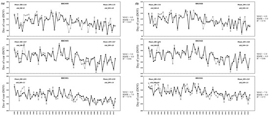
Figure 1.
Comparison between time series of observed (OB, solid line) and simulated (SM, dashed line) DOY (day of year) for phenology stages of BBCH09 (budburst), BBCH65 (flowering) and BBCH81 (veraison) for grape varieties of (a) Müller-Thurgau and (b) Riesling over 1956–2019 at Eltviller Sonnenberg. The mean (Mean_) and standard deviation (std_) of the time series for observation and simulation are labelled. MAE (days): mean absolute error; RMSE (days): root mean squared error; R2: R square.
2.5.2. Simulations of Flowering-Veraison CWSI
In the field of remote sensing, the crop water stress indicator (CWSI) has been frequently applied to assess the vine water status by calculating the difference between canopy and air temperature [75,76]. However, canopy temperature data for vineyards spanning many years and a large geographic scale remains scarce. Instead, several studies have reformulated CWSI to characterize the crop water deficit as the balance between crop water demand and water consumption, which can be simulated by many different biophysical models [30,36,77]. CWSI was computed as follows:
where ET and ETmax (sum of Emax and Tmax) are daily model outputs (see Section 2.3.2). The CWSI ranged from 0 (no stress) to 1 (severe stress), aiming to quantify the extent to which the actual ET failed to meet the potential water consumption (i.e., ETmax) from the soil-crop system, thus estimating the magnitude of water deficits experienced by plants. Simulations of CWSI enabled the integration of the effects of soil, climate and crop characteristics. CWSI was computed as the mean over the flowering-veraison phenophase (hereafter CWSI) in order to preserve its physical meaning, as suggested by Zhu et al. [36].
2.6. Software Environment
A Python-based (v3.7) simulation interface was established at the High-Performance Cluster at PIK (HPC@PIK) for grid-based crop model simulations. The interface automated dataset preprocessing (including any arbitrary soil and climate datasets) and model setup and read and wrote the simulation outputs for each target grid point. Furthermore, it used the Python message-passing interface (MPI) to parallelize the gridded simulations, thus considerably facilitating large-scale crop model applications, especially when multiple climate model projections were utilized. For data processing and result analysis, the involved python libraries were mainly numpy (v1.21.2), panda (v1.3.4) and xarray (0.19.0). To plot the results, matplotlib (v3.4.3) and cartopy (v0.20.1) were used.
3. Results
3.1. Projected Seasonal (April–October) Temperature and Precipitation Changes
The mean seasonal average temperature over the baseline period (1976–2005) shows a range between 13 °C and 16 °C, except for some high-elevation and mountainous regions and an area located in the extreme north of Germany, where these temperatures are generally below 13 °C (Figure 2a). The mean seasonal precipitation sum of the baseline period shows a range between 300 and 500 mm for most of the area, with only some high-elevation areas in the south and central regions exceeding 500 mm (Figure 2b). For climate change projections over 2041–2070, the mean seasonal temperature is projected (by ensemble median) to mainly increase by 1.5–2 °C under RCP4.5 and by 1.5–2.5 °C (a stronger increase for the southern parts of Germany) under RCP8.5 (Figure 2a). Seasonal precipitation under RCP4.5 is projected to have a marginal decrease of up to 6% for the southwestern part of the country (currently the major viticulture regions) and a slight increase of up to 5% for the remaining areas (Figure 2b). However, under RCP8.5, mean seasonal precipitation is projected to experience a widespread increase (mainly ≤10%)(Figure 2b).

Figure 2.
Ensemble median of climate model projections for the mean seasonal (April–October) (a) average temperature (°C) and (b) precipitation sum (mm) in the baseline period (1976–2005) and respective mean changes in the future period (2041–2070) under RCP4.5 and RCP8.5.
3.2. Projected Phenology (Flowering & Veraison) Changes
The projected (temporal) mean changes in the flowering stage (BBCH65), veraison stage (BBCH81) and the phenophase (BBCH65–BBCH81) are shown in Figure 3. For Müller-Thurgau, a widespread spatial pattern of advancement of 10–15 days and 15–20 days is projected for BBCH65 and BBCH81, respectively, under RCP4.5 (Figure 3a). For the same variety under RCP8.5, a prevalent pattern of earlier occurrence by 10–20 days and by 20–25 days is projected for BBH65 and BBCH81, respectively (Figure 3a). As a result, a very similar pattern of shortened BBCH65–BBCH81 phenophase is found between the two scenarios for Müller-Thurgau; mean phenophase length is mostly reduced by about one week (≤7 days) (Figure 3a). For Riesling, nearly the same spatial pattern as that for Müller-Thurgau is projected for BBCH65, i.e., a widespread advancement by 10–15 days under RCP4.5 and by 10–20 days under RCP8.5 (Figure 3b). Meanwhile, BBCH81 is projected to have a more heterogeneous spatial pattern: for some areas in the north, central and southern high-elevation regions, the advancement is limited to ≤10 days for both scenarios, whereas the remaining areas tend to have earlier occurrence by 10–20 days in RCP4.5 and by 10–25 days in RCP8.5 (Figure 3b). The resulting mean BBCH65–BBCH81 phenophase tends to be extended by up to 14 days (>14 days for some areas in RCP8.5) in those identified areas with a small advanced veraison stage and shortened by within a week (<7 days) for the remaining area (Figure 3b). Although the ensemble median of projected change is shown here, a notable spread (5th and 95th percentile) among RCMs was discovered and is presented in Figures S2–S4.
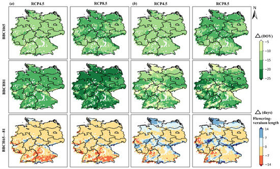
Figure 3.
Ensemble median projections for the mean DOY changes of flowering (BBCH65) and veraison stages (BBCH81) and for the BBCH65-BBCH81 phenophase between the future period (2041–2070) under RCP4.5 and RCP8.5 and the baseline period (1976–2005) for grape varieties of (a) Müller-Thurgau and (b) Riesling. For the phenophase, positive values indicate the extended period, whereas negative values denote the shortened period. DOY: day of year. Negative DOY denotes the advanced days of the phenology stages.
3.3. Projected Flowering-Veraison Temperature and Precipitation Changes
The flowering-veraison mean temperature for Müller-Thurgau is projected to mainly increase by 1–2 °C in both scenarios, despite the fact that the projected higher temperature increases by 2–2.5 °C in some central and southern plateaus and mountainous regions are more pronounced in RCP8.5 than in RCP4.5 (Figure 4a). For Riesling, the mean flowering-veraison temperature is projected to increase by 1.5–2.5 °C for the majority of areas under both scenarios, whereas, similarly to Müller-Thurgau, the projected temperature increase is higher (2–2.5 °C) in central and southern high-elevation regions (more pronounced in RCP8.5 than in RCP4.5) (Figure 4a). Concerning the flowering-veraison precipitation sum, there is a dominant spatial pattern of mean decrease by up to 15% for Müller-Thurgau under both scenarios (Figure 4b). In contrast, the distribution is more heterogeneous for Riesling. The north and central regions mainly show increases of up to 15%, whereas the rest of the study area tends to show a decrease of up to 15% under RCP4.5 (Figure 4b). In RCP8.5, a stronger (than RCP4.5) signal of increased precipitation was discovered; mean increases of 15% are predominant, whereas there are more areas with higher precipitation increases of 15–45% (Figure 4b). The ensemble median projections are shown here, while a marked spread is also found that is particularly pronounced for the projected precipitation change (Figures S5 and S6).
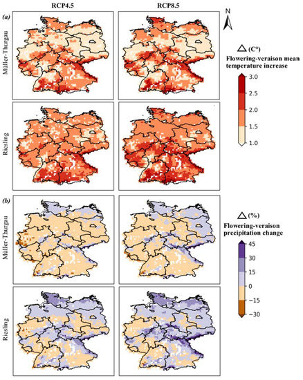
Figure 4.
Ensemble median projections for the mean (a) increased temperature (°C) and (b) change of precipitation sum (mm) in the flowering (BBCH65)-veraison (BBCH81) phenophase between the future period (2041–2070) under RCP4.5 and RCP8.5 and the baseline period (1976–2005). Positive values indicate increased temperature and precipitation in the projection period, whereas negative values denote respective decreases (where applicable).
These projected changes can be partially explained by how the shifted phenophase is exposed to projected monthly mean temperature and precipitation changes, as shown for both RCP4.5 (Figure 5a) and RCP8.5 (Figure 5b). With a higher magnitude of changes under RCP8.5, the projected monthly average temperature increase (by ensemble median) is relatively higher in summer months (July–September) than in spring months (April–June): 1.7–2.3 °C, 1.9–2.5 °C and 2.3–2.7 °C as averaged over the north, central and south regions, respectively, for summer months, as compared to those with <1.8 °C in spring months (Figure 5b). The respective (90% uncertainty range) spread of monthly temperature increase among RCMs is generally larger in April, June, September and October (up to 1.4 °C) and much smaller in July and August (<0.5 °C) (Figure 5b). For the precipitation changes (by ensemble median) in RCP8.5, the mean increases of monthly precipitation occur in April–June and in October, i.e., 8–14% in the north, 5–12% in the central and southern regions, whereas the changes in July–September are more uncertain, as smaller mean changes with a larger spread are generally found in these months than in the other months (Figure 5b). The flowering-veraison phenophase of both varieties is shifted earlier, but the two varieties tend to have different exposures to projected monthly meteorological changes. For Müller-Thurgau, the shifted phenophase is accompanied by reduced length of the phase (Figure 3a), spanning from mid-June to early August for all three regions, thus being substantially exposed to summer months with increased mean temperature and uncertain precipitation changes (although this may partially capture the mean increased June precipitation) (Figure 5b). For Riesling, the shifted phenophase mainly spans from mid-June to late August but is accompanied by varying lengths of phenophase across all regions (Figure 3b). Thus, Riesling is more exposed to summer months as compared to Müller-Thurgau (Figure 5b). A similar pattern is also projected for RCP4.5 (Figure 5a) but with an overall smaller magnitude of changes as compared to RCP8.5 (Figure 5b).
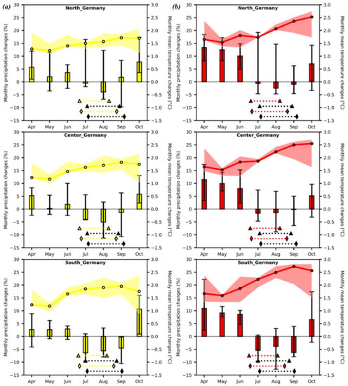
Figure 5.
Projected monthly average temperature changes (°C) (in line plot) and precipitation sum changes (%) (in bar plot) over the growing season (April–October) for the future period (2041–2070) under (a) RCP4.5 (yellow) and (b) RCP8.5 (red) as compared to the baseline period (1976—2005) in northern (Latitude 52°–55°), central (Latitude 50°–52°) and southern (Latitude 47°–50°) Germany. In the line plot, the lines represent regional mean values with the respective colour band indicating their 90% uncertainty range among RCMs. In the bar plot, bars indicate the regional mean values with the respective error bars indicating their 90% uncertainty range among RCMs. The regional mean flowering stage and veraison stage are also shown for Müller-Thurgau (triangular) and Riesling (diamond). Note that for the same variety in each subplot, the phenology symbols occurring earlier correspond to the flowering stage, and the next symbol is the veraison stage. The phenology symbols with black, yellow and red are for the baseline, RCP4.5 and RCP8.5, respectively.
3.4. Projected Impacts of Climate Change on Flowering-Veraison CWSI
The mean flowering-veraison CWSI is projected to have a similar pattern for the two varieties, in which a mean increase of up to 15% is projected for most of the area (including the major winegrowing regions) in both scenarios, except for the northeastern and central areas, which are projected to decrease by up to 15% (Figure 6). However, there is a more consistent increase (by ensemble median) of CWSI in RCP4.5 than in RCP8.5, i.e., RCP8.5 projections show more areas (mainly in the northeastern and central regions) with decreased CWSI (Figure 6). However, these results are subject to considerable uncertainties, as the lower (5th) percentile simulations of RCMs (both varieties) tend to show widespread mean reductions of CWSI of up to 15% in RCP8.5, with a more heterogeneous pattern for RCP4.5 (Figure 6). Conversely, the higher (95th) percentile simulations of RCMs (both varieties) largely show a consistent spatial pattern of mean increased CWSI of up to 30% in both scenarios (Figure 6). The individual model projections are provided in Appendix A. Although both varieties tend to have a similar spatial pattern for projected CWSI changes, they differ in their projections of ETmax and ET (CWSI components). For Müller-Thurgau, both the sum of ETmax and that of ET over the flowering-veraison phase tend to show widespread reductions by up to 15% (relative to baseline), as indicated by both the ensemble median and 5th/95th percentile (Figures S7 and S8). In contrast, for Riesling, both ETmax and ET sums primarily show an increase by up to 15% (some areas >30%) over most of Germany, whereas some areas show a decrease by up to 15% (Figures S7 and S8).
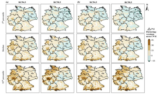
Figure 6.
Projected changes (%) of mean crop water stress indicator (CWSI) for the flowering (BBCH65)-veraison (BBCH81) phenophase for (a) Müller-Thurgau and (b) Riesling between the future period (2041–2070) under RCP4.5 and RCP8.5 and the baseline period (1976–2005). The 5th percentile, median and 95th percentile of simulations under different climate models are shown. Positive values indicate increased CWSI (intensified water stress), whereas negative values denote respective reductions (alleviated water stress).
4. Discussion
4.1. Evaluation of Model Performance for Phenology Simulations
Accurate phenology simulations are critical to assess the water deficits calculated over the flowering-veraison phase. First, the model was calibrated to simulate the flowering (BBCH65) and veraison (BBCH81) stages using a long time series (1956–2019) of observed data for the two varieties. Satisfactory model performance was obtained for both varieties, with a mean bias of only 1–2 days and well-reproduced interannual variability (Figure 1). When the model was further driven by gridded historical RCM simulations, it is corroborated that the simulated regional mean DOY of flowering and of veraison (Figure 5) agree well with local observed mean timings (mean over 1968–2010) on 22th June and 11 th August (mean 50 day interval) for Müller-Thurgau and on 24th June and 24th August (mean 61 day interval) for Riesling [78].
4.2. Phenology Projections
With increased temperatures under climate change projections, the results indicate generally advanced phenology stages, although a greater advancement of phenology was discovered for RCP8.5 than for RCP4.5 (Figure 3). A similar magnitude of advancement (10–20 days across scenarios) was found for the flowering stage between varieties, whereas a slightly greater advancement of veraison is projected for Müller-Thurgau (15–25 days across scenarios) than for Riesling (10–25 days across scenarios) (Figure 3). In comparison, Molitor and Junk [19] projected advanced flowering and veraison stages by 9 and 10 days for Müller-Thurgau and by 9 and 11 days for Riesling, respectively, over 2031–2060 under the A1B (comparable to RCP6.0) emission scenario in Luxembourg. The relatively higher magnitude of advancement in our study can be attributed to projected higher seasonal mean temperature increases by 1.5–2.5 °C (depending on the scenario) compared with <1.5°C projected by Molitor and Junk [19]. Many studies suggest that differences in the magnitude of earlier occurrence of simulated phenology stages under global warming can be explained by differences in the studied varieties, the phenology models applied and the extent of temperature increases [19,31,45,79]. Moreover, smaller advanced veraison stages (≤ 10 days) of Riesling (under both scenarios) are identified in areas with either a cooler reference climate (Figure 2a) or mountainous terrain (>400 m) (Figure S1). A particularly higher temperature increase is projected in these areas (Figure 4a). Hence, there could have been a delay in the veraison date due to projected high temperatures (mainly in August for Riesling) that frequently exceed the defined upper threshold (37 °C) above which phenology development is halted [35]. As a result of such asymmetric phenology advancements (a greater advancement for flowering than for veraison stage), the flowering-veraison phenophase in those areas is extended by up to 14 days (some >14 days under RCP8.5) (Figure 3b). In Alsace (France), delayed veraison projections with increased temperature were also obtained for Riesling using a similar GDD model and with a 33 °C upper threshold as compared with projections without a threshold [79]. Similarly, Ramos et al. [31] also report delayed phenology timing under the hottest conditions for vineyard plots located at a high elevation compared to plots at a low elevation.
4.3. Projected Temperature and Precipitation Changes
The projected higher magnitude of seasonal temperature increase in RCP8.5 than in RCP4.5 (Figure 2) is expected, since RCP8.5 assumed a much higher thermal forcing than that in RCP4.5 [52,53]. For seasonal precipitation projections, there is a widespread in-crease in RCP8.5 compared with more uncertain changes (−6% to 5%) in RCP4.5 (Figure 2). Similar findings were also obtained in several other studies [9,51,80,81]. For instance, Dietrich et al. [80] showed the projected mean annual precipitation changes for Germany over 2041–2050 (relative to 1971–2000) are of −2.2% and 6.7% in RCP4.5 and RCP8.5, respectively, for which a higher magnitude of monthly precipitation increase was also found in RCP8.5 than in RCP4.5, spanning most of the months. On the other hand, the projected changes in mean temperature and precipitation sum during the flowering-veraison phase (Figure 4) should be interpreted with care, as they are simultaneously affected by three factors: (1) advanced phenology with shifted phenophase towards the cooler spring season for both varieties; (2) shortened or prolonged phenophase, depending on the variety (Figure 3); (3) different exposures to projected monthly mean temperature and precipitation changes, depending on the variety (Figure 5). However, it is beyond the scope of this article to disentangle each of these factors and quantify the contribution of each of them to the projected changes across Germany. Results show Riesling will remain a late-ripening variety as compared to Müller-Thurgau under future climate conditions, although differences in the flowering stage remain small (Figure 5). The gap between the veraison stage for Müller-Thurgau and Riesling is enlarged in the future period under both scenarios (Figure 5). Therefore, Riesling is more exposed to the high-temperature increase in August, whereas the monthly precipitation change is more uncertain (Figure 5). The extended flowering-veraison phenophase (Figure 3b) can be assumed as the major factor (compared to the other two factors) in the projected increases of flowering-veraison precipitation for Riesling (Figure 4b). The decreased precipitation for Müller-Thurgau (Figure 4b) can be mainly attributed to the shortened flowering-veraison phase (Figure 3a). Nevertheless, it should be emphasized that small absolute changes in precipitation amount may appear as large percentage changes, particularly given the relatively small cumulative precipitation amount of the flowering-veraison phase. As Molitor and Junk [19] demonstrated, temperature changes in calendar-based time frames cannot reveal the actual temperature changes in a specific development stage. In this study, the changes for a phase-dependent meteorological condition were assessed; however, this approach is complex, especially when analysing a large geographic area.
4.4. Projected Changes of Flowering-Veraison Water Deficits
The impacts of projected climate change on the total flowering-veraison ETmax and ET tend to differ between the two varieties (Figures S7 and S8), which represent the water demand and consumption of the investigated soil-crop system, respectively [36,61,65]. For Müller-Thurgau, the overall reduction in the sum of ETmax in the flowering-verasion phase (Figure S7) can be mainly attributed to the reduced length of the phenophase (Figure 3a), reduced potential evapotranspiration due to shifted phenophase towards a cooler spring and projected flowering-veraison temperature increase (Figure 4a). For Riesling, the increased sum of ETmax (Figure S7) is primarily due to the combined effect of an extended flowering-veraison phase (Figure 3b), higher flowering-veraison (relative to Müller-Thurgau) temperature increase (Figure 4a) and shifted phenophase towards the spring when potential evapotranspiration is lower. For Riesling, we assume that the length of phenophase plays a major role in determining the changes in ETmax, as the identified areas with decreased ETmax (Figure S7) are generally consistent with areas with a shortened phenophase (Figure 3b). Besides, it should be noted that the effects of elevated CO2 levels (in two scenarios) on reducing ETmax (mainly via Tmax) have already been explicitly considered by STICS for both varieties under the two scenarios investigated [35,65]. The ET pattern generally follows that of ETmax but is more difficult to interpret, as it additionally interacts with projected precipitation changes and plant growth response (e.g., heat stress limitations) [35]. As a result, both varieties show a similar spatial pattern of projected CWSI changes (Figure 6), partly because of the offset of changes between ETmax and ET for each variety (Figures S7 and S8). An overall increased CWSI by up to 15% (captured by the ensemble median) is obtained over most of the study area for both varieties (Figure 6). This result is consistent with results reported by Hofmann et al. [13] and Fraga et al. [42]. At the vineyard level, Hofmann et al. [13] projected a significantly increased frequency of the occurrence of severe drought stress over a fixed calendar period (1st May–30th September) for Riesling by using a different vineyard model under multiple RCMs. At a large geographic scale, Fraga et al. [42] suggested that vine water stress conditions for Pinot noir from fruit set until maturity are projected to have a particularly high increase in central European wine regions.
Assessing potential climate change impacts can help support winegrowers to implement suitable adaptations for improved viticulture management. The effect of water deficits on red wine quality is well documented; except for situations where it is particularly severe, quality is increased [22,82]. The effect of water deficits on white wine quality is less well documented. The threshold of water deficit where white wine quality decreases is probably reached earlier compared to that of red wine, although recent researches suggest that mild levels of water deficit increase the content of some key aromatic compounds in white wines [82,83]. Therefore, in areas with projected intensifications of CWSI, shifting to red varieties might be a good option, e.g., replacing the declining variety Müller-Thurgau with Pinot noir, Cabernet-Sauvignon, Syrah or Tempranillo [45], as their quality can benefit from increased water deficits [22,29]. This is especially relevant for some current winegrowing regions in the southwest of Germany, where an upper (95th) percentile simulation potentially shows a strong signal of intensified water deficit by around 30% (some areas even >45%) (Figure 5). On the other hand, the identified areas in the northeastern and central regions with alleviated CWSI (by up to 15%) should preferentially be planted with white varieties (Figure 5). Several other adaptation strategies can also be implemented to reduce the potentially detrimental effects of excessive water deficit stress. Grafting vines onto more drought-resistant rootstocks is a cost-effective and environmentally friendly adaptation to increased drought [84]. Predominant rootstocks currently used in Germany are V. berlandieri × V. riparia siblings (e.g., SO4, 5BB, 125 AA). Rootstocks from the family V. berlandieri × V. rupestris (in particular 110R) are much more drought-resistant [85]. Substantial differences also exist among grapevine varieties regarding their tolerance to drought [86,87]. Reduced planting density also relieves water deficit in vineyards because it decreases ET [88]. Vines are currently dry-farmed in Germany, and implementing irrigation can also be considered, in particular to limit potential yield losses [14,16]. However, irrigation has a high environmental cost because it significantly increases the blue water footprint of wine production [89] and should be used as the last adaptation strategy [7].
4.5. Strengths and Limitations
Potential climate change effects on water deficit/scarcity of a drought-sensitive period (flowering-veraison) were assessed for two main German varieties, i.e., Müller-Thurgau and Riesling. The viticulture model employed in this study is one of few models that can capture the interplay between phenology timing and vine growth response to drought stress [35,37,59]. Rising temperature alone impacts both phenology and plant water demand, whereas changes in the precipitation distribution during the phenophase additionally affect soil water availability [7]. A holistic approach was implemented to address climate change impacts, considering vine development to projected changes not only in temperature and precipitation but also the covariance between other climatic variables (radiation, wind speed and humidity, i.e., these variables can additionally modify vine water demand). Besides, we specifically analysed drought risk during an important phenophase instead of the calendar season, which can produce more relevant information for viticulturalists and winemakers. Furthermore, our findings demonstrate that phenophase-dependent water deficits are affected by multiple and correlated factors, among which changes in the length of the phenophase may play an important role. The results obtained in this study can be applied to any variety with similar precocity for flowering and veraison as Müller-Thurgau (early-ripening) and Riesling (late-ripening). For example, the flowering and veraison dates of Riesling are comparable to those of Merlot [49,90], so the obtained result for Riesling might be applied to Merlot as well.
Nevertheless, when assessing climate change impacts on viticulture, some limitations should be considered [4]. Firstly, although the projected magnitude of increase in summer temperature is quite consistent across RCMs, considerable uncertainties are found in projected summer-month precipitation changes (Figure 5). The spread among RCMs is still considerable when simulating the flowering-veraison CWSI (Figure 6, Appendix A). This again illustrates the complexity of climate change impact assessment; projections already diverge substantially for mean changes, and the assessment of interannual variability is even more difficult. Secondly, only one grapevine model was used in this study, and there is a clear need to consider potential variability in simulations through the use of multiple crop models in impact assessment [32,34,91]. This point mainly concerns the question of how reliable the S-W module (Section 2.3.2) is for simulation of ETmax and ET [65]. Since the two varieties are only characterized by their differences in phenology (Table S1), additional lysimeter measurements for these water use variables could be useful to verify the model simulations. Lastly, quantitative information about natural variation and in situ vineyard management is lacking, which does not allow for consideration of the effects of fine-scale topographical niches and microclimate variations, which can potentially buffer adverse climate effects [4,92].
Consequently, the present framework for impact analysis of climate change is primarily based on several gridded products, either assimilating a large sample of in situ observations, such as the EU-SoilHydroGrids [44], or utilizing regional climate modelling from high-resolution, bias-adjusted RCMs from the EURO–CORDEX initiative. Further steps can consider using a crop model (such as STICS) to assimilate remote-sensed products during calibration, such as LAI [93] and soil water content [94], in order to obtain parameter values that can better represent vine growth response to seasonal water deficits. This can aid in reducing simulation uncertainties both in the present and in future climates, thus improving the reliability of climate change impact assessments.
Supplementary Materials
The following supporting information can be downloaded at: https://www.mdpi.com/article/10.3390/rs14061519/s1. Figure S1: Elevation and slope (>15°) map in Germany based on the European Digital Elevation Model (EU-DEM, v.1.1); Figure S2–S6: The 5th and 95th percentile (spread) of ensemble simulations for the flowering stage (BBCH65), veraison stage (BBCH81), flowering-veraison (BBCH65–BBCH81) phenophase, flowering-veraison (BBCH65–BBCH81) average temperature (°C) and flowering-veraison (BBCH65–BBCH81) precipitation sum (mm). Figure S7–S8: Projected (temporal) mean changes (%) of maximum evapotranspiration (ETmax) and actual evapotranspiration (ET) sum (mm) during the flowering-veraison (BBCH65–BBCH81) phenophase, as indicated by the 5th percentile, median and 95th percentile of ensemble simulations. Table S1: Calibrated STICS model parameter values for simulating BBCH09, BBCH65 and BBCH81 over 1956—2019 at Eltviller Sonnenberg for Müller-Thurgau and Riesling grape varieties.
Author Contributions
Conceptualization, C.Y., C.M., M.S.D.A.J., S.C.-A., M.M., L.L., A.T.-M., D.M., J.J., H.F., C.v.L. and J.A.S.; methodology, C.Y. and C.M.; software, C.Y., C.M. and M.S.D.A.J.; validation, C.Y., C.M., M.S.D.A.J., S.C.-A., M.M., L.L., A.T.-M., D.M., J.J., H.F., C.v.L. and J.A.S.; formal analysis, C.Y., C.M., M.S.D.A.J., S.C.-A., M.M., L.L., A.T.-M., D.M., J.J., H.F., C.v.L. and J.A.S.; investigation, C.Y., C.M., M.S.D.A.J., S.C.-A., M.M., L.L., A.T.-M., D.M., J.J., H.F., C.v.L. and J.A.S.; resources, C.Y. and C.M.; data curation, C.Y.; writing—original draft preparation, C.Y.; writing—review and editing, C.Y., C.M., M.S.D.A.J., S.C.-A., M.M., L.L., A.T.-M., D.M., J.J., H.F., C.v.L. and J.A.S.; visualization, C.Y. and C.M.; supervision, C.Y., C.M., M.S.D.A.J., S.C.-A., M.M., L.L., A.T.-M., D.M., J.J., H.F., C.v.L. and J.A.S.; project administration, J.A.S.; funding acquisition, C.Y., C.M., S.C.-A., M.M., L.L., A.T.-M., D.M., J.J., H.F., C.v.L. and J.A.S. All authors have read and agreed to the published version of the manuscript.
Funding
This research was funded by the Clim4Vitis project, “Climate change impact mitigation for European viticulture: knowledge transfer for an integrated approach”, funded by the European Union’s Horizon 2020 Research and Innovation Programme under grant agreement no. 810176. This research was also supported by the Portuguese Foundation for Science and Technology (FCT) under project UIDB/04033/2020. This work also received funding under the framework of the CHAPEL project, as funded by the Ministère de l’Environnement, du Climat et du Développement of Luxembourg. We also thank the CoaClimateRisk project (COA/CAC/0030/2019) of the FCT.
Institutional Review Board Statement
Not applicable.
Informed Consent Statement
Not applicable.
Data Availability Statement
Different regional climate model (RCM) simulations produced within the EURO–CORDEX initiative can be accessed at https://www.euro-cordex.net/ (accessed on 19 March 2022). The freely available software STICS can be accessed and downloaded at https://www6.paca.inrae.fr/stics_eng/Download (accessed on 19 March 2022). The FAO Harmonized World Soil Database (HWSD) can be found at https://www.fao.org/soils-portal/data-hub/soil-maps-and-databases/harmonized-world-soil-database-v12/en/ (accessed on 19 March 2022). The EU-SoilHydroGrids dataset can be found at https://esdac.jrc.ec.europa.eu/content/3d-soil-hydraulic-database-europe-1-km-and-250-m-resolution (accessed on 19 March 2022). The European Digital Elevation Model dataset can be found at https://land.copernicus.eu/imagery-in-situ/eu-dem/eu-dem-v1.1?tab=metadata (accessed on 19 March 2022).
Acknowledgments
We acknowledge data provisions from Bernd Neckerauer, Dezernat Weinbau, Regierungspräsidiums Darmstatt and Copernicus service.
Conflicts of Interest
The authors declare no conflict of interests.
Appendix A
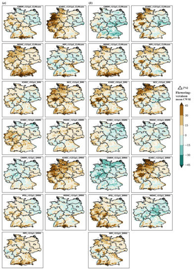
Figure A1.
Individual model projections for changes (%) in mean crop water stress indicator (CWSI) during the flowering (BBCH65)-veraison (BBCH81) phenophase for the future period (2041–2070) under (a) RCP4.5 and (b) RCP8.5 as compared to the baseline period (1976–2005) for Müller-Thurgau. Positive values indicate increased CWSI (intensified water stress), whereas negative values denote respective reductions (alleviated water stress).
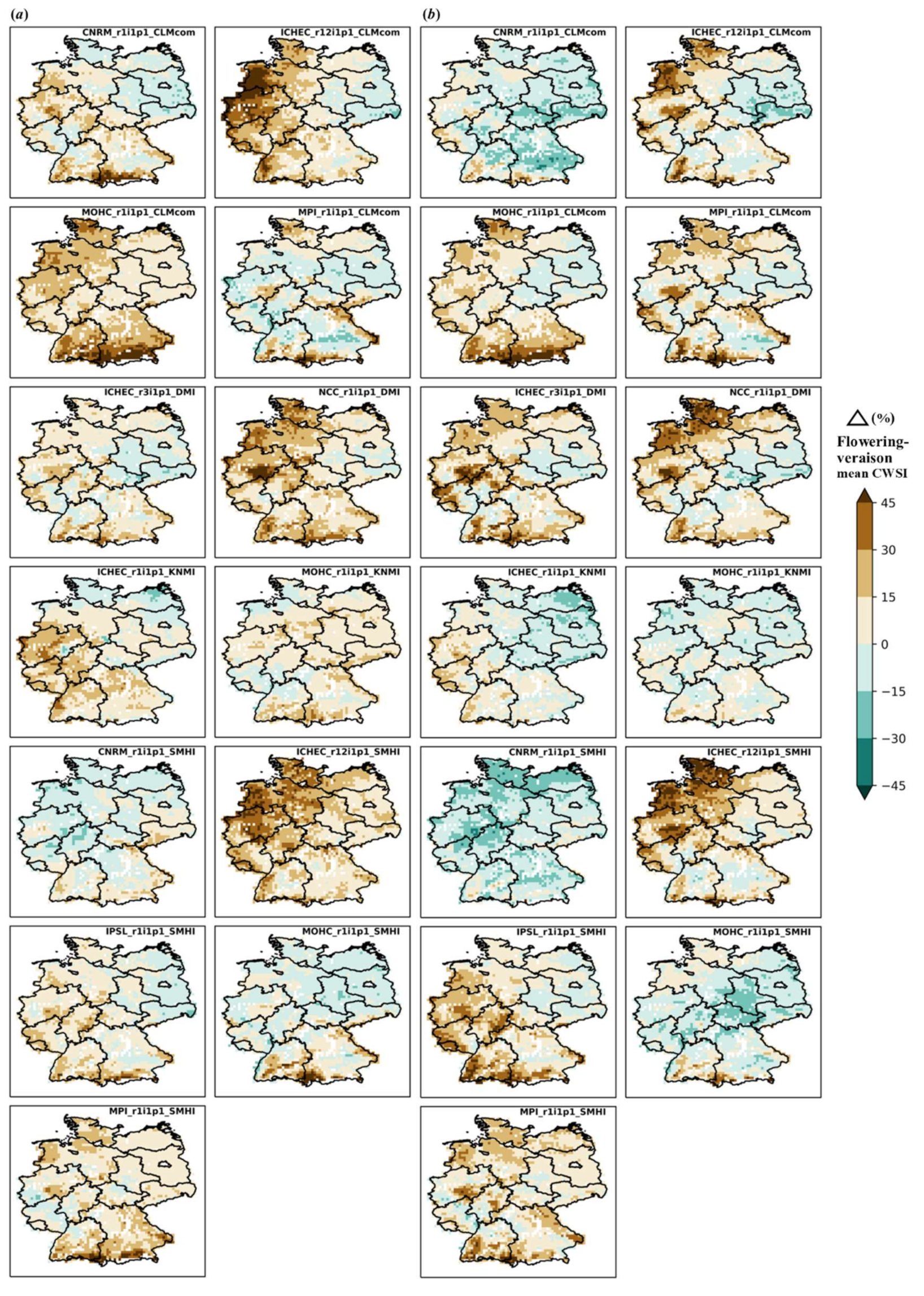
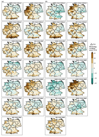
Figure A2.
Individual model projections for changes (%) in mean crop water stress indicator (CWSI) during the flowering (BBCH65)-veraison (BBCH81) phenophase for the future period (2041–2070) under (a) RCP4.5 and (b) RCP8.5 as compared to the baseline period (1976–2005) for Riesling. Positive values indicate increased CWSI (intensified water stress), whereas negative values denote respective reductions (alleviated water stress).

References
- OIV. State of the Vitiviniculture World Market. 2021. Available online: https://www.oiv.int/en/technical-standards-and-documents/statistical-analysis/state-of-vitiviniculture (accessed on 1 June 2021).
- IPCC. Climate Change 2021: The Physical Science Basis. Contribution of Working Group I to the Sixth Assessment Report of the Intergovernmental Panel on Climate Change; IPCC: Geneva, Switzerland, 2021. [Google Scholar]
- Santos, J.A.; Fraga, H.; Malheiro, A.C.; Moutinho-Pereira, J.; Dinis, L.T.; Correia, C.; Moriondo, M.; Leolini, L.; Dibari, C.; Costafreda-Aumedes, S.; et al. A review of the potential climate change impacts and adaptation options for European viticulture. Appl. Sci. 2020, 10, 3092. [Google Scholar] [CrossRef]
- Mosedale, J.R.; Abernethy, K.E.; Smart, R.E.; Wilson, R.J.; Maclean, I.M.D. Climate change impacts and adaptive strategies: Lessons from the grapevine. Glob. Change Biol. 2016, 22, 3814–3828. [Google Scholar] [CrossRef] [Green Version]
- Leolini, L.; Moriondo, M.; Fila, G.; Costafreda-Aumedes, S.; Ferrise, R.; Bindi, M. Late spring frost impacts on future grapevine distribution in Europe. Field Crops Res. 2018, 222, 197–208. [Google Scholar] [CrossRef]
- Jones, G.V.; White, M.A.; Cooper, O.R.; Storchmann, K. Climate change and global wine quality. Clim. Change 2005, 73, 319–343. [Google Scholar] [CrossRef]
- Van Leeuwen, C.; Destrac-Irvine, A.; Dubernet, M.; Duchêne, E.; Gowdy, M.; Marguerit, E.; Pieri, P.; Parker, A.; de Rességuier, L.; Ollat, N. An Update on the Impact of Climate Change in Viticulture and Potential Adaptations. Agronomy 2019, 9, 514. [Google Scholar] [CrossRef] [Green Version]
- Moriondo, M.; Jones, G.V.; Bois, B.; Dibari, C.; Ferrise, R.; Trombi, G.; Bindi, M. Projected shifts of wine regions in response to climate change. Clim. Change 2013, 119, 825–839. [Google Scholar] [CrossRef]
- Cardell, M.F.; Amengual, A.; Romero, R. Future effects of climate change on the suitability of wine grape production across Europe. Reg. Environ. Change 2019, 19, 2299–2310. [Google Scholar] [CrossRef]
- Hannah, L.; Roehrdanz, P.R.; Ikegami, M.; Shepard, A.V.; Shaw, M.R.; Tabor, G.; Zhi, L.; Marquet, P.A.; Hijmans, R.J. Climate change, wine, and conservation. Proc. Natl. Acad. Sci. USA 2013, 110, 6907–6912. [Google Scholar] [CrossRef] [Green Version]
- Neumann, P.; Matzarakis, A. Viticulture in southwest Germany under climate change conditions. Clim. Res. 2011, 47, 161–169. [Google Scholar] [CrossRef]
- Van Leeuwen, C.; Seguin, G. The concept of terroir in viticulture. J. Wine Res. 2006, 17, 1–10. [Google Scholar] [CrossRef]
- Hofmann, M.; Lux, R.; Schultz, H.R. Constructing a framework for risk analyses of climate change effects on the water budget of differently sloped vineyards with a numeric simulation using the Monte Carlo method coupled to a water balance model. Front. Plant Sci. 2014, 5, 645. [Google Scholar] [CrossRef] [PubMed] [Green Version]
- Chaves, M.M.; Zarrouk, O.; Francisco, R.; Costa, J.M.; Santos, T.; Regalado, A.P.; Rodrigues, M.L.; Lopes, C.M. Grapevine under deficit irrigation: Hints from physiological and molecular data. Ann. Bot. 2010, 105, 661–676. [Google Scholar] [CrossRef] [Green Version]
- Ramos, M.C.; Martínez-Casasnovas, J.A. Soil water variability and its influence on transpirable soil water fraction with two grape varieties under different rainfall regimes. Agric. Ecosyst. Environ. 2014, 185, 253–262. [Google Scholar] [CrossRef]
- Intrigliolo, D.S.; Pérez, D.; Risco, D.; Yeves, A.; Castel, J.R. Yield components and grape composition responses to seasonal water deficits in Tempranillo grapevines. Irrig. Sci. 2012, 30, 339–349. [Google Scholar] [CrossRef]
- Ramos, M.C.; Pérez-Álvarez, E.P.; Peregrina, F.; Martínez de Toda, F. Relationships between grape composition of Tempranillo variety and available soil water and water stress under different weather conditions. Sci. Hortic. Amst. 2020, 262, 109063. [Google Scholar] [CrossRef]
- Schultz, H.R.; Stoll, M. Some critical issues in environmental physiology of grapevines: Future challenges and current limitations. Aust. J. Grape Wine Res. 2010, 16, 4–24. [Google Scholar] [CrossRef]
- Molitor, D.; Junk, J. Climate change is implicating a two-fold impact on air temperature increase in the ripening period under the conditions of the Luxembourgish grapegrowing region. OENO One 2019, 53. [Google Scholar] [CrossRef]
- Junk, J.; Goergen, K.; Krein, A. Future Heat Waves in Different European Capitals Based on Climate Change Indicators. Int. J. Environ. Res. Public Health 2019, 16, 3959. [Google Scholar] [CrossRef] [PubMed] [Green Version]
- Fraga, H.; Molitor, D.; Leolini, L.; Santos, J.A. What Is the Impact of Heatwaves on European Viticulture? A Modelling Assessment. Appl. Sci. 2020, 10, 3030. [Google Scholar] [CrossRef]
- van Leeuwen, C.; Trégoat, O.; Choné, X.; Bois, B.; Pernet, D.; Gaudillère, J.-P. Vine water status is a key factor in grape ripening and vintage quality for red Bordeaux wine. How can it be assessed for vineyard management purposes? J. Int. Sci. Vigne Vin. 2009, 43, 121–134. [Google Scholar] [CrossRef]
- Van Leeuwen, C.; Roby, J.-P.; de Rességuier, L. Soil-related terroir factors: A review. OENO One 2018, 52, 173–188. [Google Scholar] [CrossRef] [Green Version]
- Gambetta, G.A.; Herrera, J.C.; Dayer, S.; Feng, Q.; Hochberg, U.; Castellarin, S.D. The physiology of drought stress in grapevine: Towards an integrative definition of drought tolerance. J. Exp. Bot. 2020, 71, 4658–4676. [Google Scholar] [CrossRef] [PubMed]
- Roby, G.; Harbertson, J.F.; Adams, D.A.; Matthews, M.A. Berry size and vine water deficits as factors in winegrape composition: Anthocyanins and tannins. Aust. J. Grape Wine Res. 2004, 10, 100–107. [Google Scholar] [CrossRef]
- Triolo, R.; Roby, J.P.; Pisciotta, A.; Di Lorenzo, R.; van Leeuwen, C. Impact of vine water status on berry mass and berry tissue development of Cabernet franc (Vitis vinifera L.), assessed at berry level. J. Sci. Food Agric. 2019, 99, 5711–5719. [Google Scholar] [CrossRef]
- Guilpart, N.; Metay, A.; Gary, C. Grapevine bud fertility and number of berries per bunch are determined by water and nitrogen stress around flowering in the previous year. Eur. J. Agron. 2014, 54, 9–20. [Google Scholar] [CrossRef]
- Ojeda, H.; Deloire, A.; Carbonneau, A. Influence of water deficits on grape berry growth. Vitis 2001, 40, 141–146. [Google Scholar] [CrossRef]
- Ojeda, H.; Andary, C.; Kraeva, E.; Carbonneau, A.; Deloire, A. Influence of Pre- and Postveraison Water Deficit on Synthesis and Concentration of Skin Phenolic Compounds during Berry Growth of Vitis vinifera cv. Shiraz. Am. J. Enol. Vitic. 2002, 53, 261–267. [Google Scholar]
- Yang, C.; Menz, C.; Fraga, H.; Costafreda-Aumedes, S.; Leolini, L.; Ramos, M.C.; Molitor, D.; van Leeuwen, C.; Santos, J.A. Assessing the grapevine crop water stress indicator over the flowering-veraison phase and the potential yield lose rate in important European wine regions. Agric. Water Manag. 2022, 261, 107349. [Google Scholar] [CrossRef]
- Ramos, M.C.; Go, D.T.H.C.; Castro, S. Spatial and temporal variability of cv. Tempranillo response within the Toro DO (Spain) and projected changes under climate change. OENO One 2021, 55, 349–366. [Google Scholar] [CrossRef]
- Tao, F.; Palosuo, T.; Rötter, R.P.; Díaz-Ambrona, C.G.H.; Inés Mínguez, M.; Semenov, M.A.; Kersebaum, K.C.; Cammarano, D.; Specka, X.; Nendel, C.; et al. Why do crop models diverge substantially in climate impact projections? A comprehensive analysis based on eight barley crop models. Agric. For. Meteorol. 2020, 281, 107851. [Google Scholar] [CrossRef]
- Rötter, R.P.; Hoffmann, M.P.; Koch, M.; Müller, C. Progress in modelling agricultural impacts of and adaptations to climate change. Curr. Opin. Plant Biol. 2018, 45, 255–261. [Google Scholar] [CrossRef] [PubMed]
- Rosenzweig, C.; Jones, J.W.; Hatfield, J.L.; Ruane, A.C.; Boote, K.J.; Thorburn, P.; Antle, J.M.; Nelson, G.C.; Porter, C.; Janssen, S.; et al. The Agricultural Model Intercomparison and Improvement Project (AgMIP): Protocols and pilot studies. Agric. For. Meteorol. 2013, 170, 166–182. [Google Scholar] [CrossRef] [Green Version]
- Brisson, N.; Launay, M.; Mary, B.; Beaudoin, N. Conceptual Basis, Formalisations and Parameterization of the STICS Crop Model; Editions Quae: Versailles, France, 2009; ISBN 2759201694. [Google Scholar]
- Zhu, X.; Xu, K.; Liu, Y.; Guo, R.; Chen, L. Assessing the vulnerability and risk of maize to drought in China based on the AquaCrop model. Agric. Syst. 2021, 189, 103040. [Google Scholar] [CrossRef]
- García de Cortázar-Atauri, I. Adaptation du Modèle STICS à la Vigne (Vitis vinifera L.). Utilisation dans le Cadre d’Une Étude d’Impact du Changement Climatique à l’Échelle de la France. Ph.D. Thesis, l’Ecole Nationale Superieure Agronomique de Montpellier, Montpellier, France, 2006. [Google Scholar]
- Fraga, H.; Costa, R.; Moutinho-Pereira, J.; Correia, C.M.; Dinis, L.T.; Gonçalves, I.; Silvestre, J.; Eiras-Dias, J.; Malheiro, A.C.; Santos, J.A. Modeling phenology, water status, and yield components of three Portuguese grapevines using the STICS crop model. Am. J. Enol. Vitic. 2015. [Google Scholar] [CrossRef]
- Valdés-Gómez, H.; Celette, F.; García de Cortázar-Atauri, I.; Jara-Rojas, F.; Ortega-Farías, S.; Gary, C. Modelling soil water content and grapevine growth and development with the stics crop-soil model under two different water management strategies. J. Int. Sci. Vigne Vin. 2009, 43, 13–28. [Google Scholar] [CrossRef] [Green Version]
- Coucheney, E.; Buis, S.; Launay, M.; Constantin, J.; Mary, B.; García de Cortázar-Atauri, I.; Ripoche, D.; Beaudoin, N.; Ruget, F.; Andrianarisoa, K.S.; et al. Accuracy, robustness and behavior of the STICS soil–crop model for plant, water and nitrogen outputs: Evaluation over a wide range of agro-environmental conditions in France. Environ. Model. Softw. 2015, 64, 177–190. [Google Scholar] [CrossRef]
- Ajaz, A.; Taghvaeian, S.; Khand, K.; Gowda, P.H.; Moorhead, J.E. Development and Evaluation of an Agricultural Drought Index by Harnessing Soil Moisture and Weather Data. Water 2019, 11, 1375. [Google Scholar] [CrossRef] [Green Version]
- Fraga, H.; García de Cortázar Atauri, I.; Malheiro, A.C.; Santos, J.A. Modelling climate change impacts on viticultural yield, phenology and stress conditions in Europe. Glob. Change Biol. 2016, 22, 3774–3788. [Google Scholar] [CrossRef]
- Lange, S. Trend-preserving bias adjustment and statistical downscaling with ISIMIP3BASD (v1.0). Geosci. Model Dev. 2019, 12, 3055–3070. [Google Scholar] [CrossRef] [Green Version]
- Tóth, B.; Weynants, M.; Pásztor, L.; Hengl, T. 3D soil hydraulic database of Europe at 250 m resolution. Hydrol. Process. 2017, 31, 2662–2666. [Google Scholar] [CrossRef] [Green Version]
- Koch, B.; Oehl, F. Climate change favors grapevine production in temperate zones. Agric. Sci. 2018, 9, 247–263. [Google Scholar] [CrossRef] [Green Version]
- Molitor, D.; Schultz, M.; Mannes, R.; Pallez-Barthel, M.; Hoffmann, L.; Beyer, M. Semi-Minimal Pruned Hedge: A Potential Climate Change Adaptation Strategy in Viticulture. Agronomy 2019, 9, 173. [Google Scholar] [CrossRef] [Green Version]
- Schäfer, J.; Friedel, M.; Molitor, D.; Stoll, M. Semi-Minimal-Pruned Hedge (SMPH) as a Climate Change Adaptation Strategy: Impact of Different Yield Regulation Approaches on Vegetative and Generative Development, Maturity Progress and Grape Quality in Riesling. Appl. Sci. 2021, 11, 3304. [Google Scholar] [CrossRef]
- Parker, A.K.; García de Cortázar-Atauri, I.; Gény, L.; Spring, J.L.; Destrac, A.; Schultz, H.; Molitor, D.; Lacombe, T.; Graça, A.; Monamy, C.; et al. Temperature-based grapevine sugar ripeness modelling for a wide range of Vitis vinifera L. cultivars. Agric. For. Meteorol. 2020, 285–286, 107902. [Google Scholar] [CrossRef]
- Molitor, D.; Fraga, H.; Junk, J. UniPhen—A unified high resolution model approach to simulate the phenological development of a broad range of grape cultivars as well as a potential new bioclimatic indicator. Agric. For. Meteorol. 2020, 291, 108024. [Google Scholar] [CrossRef]
- Anderson, K.; Nelgen, S. Which Winegrape Varieties Are Grown Where? A Global Empirical Picture; University of Adelaide Press: Adelaide, Australia, 2013; ISBN 978-1-922064-68-4. [Google Scholar]
- Jacob, D.; Petersen, J.; Eggert, B.; Alias, A.; Christensen, O.B.; Bouwer, L.M.; Braun, A.; Colette, A.; Déqué, M.; Georgievski, G.; et al. EURO-CORDEX: New high-resolution climate change projections for European impact research. Reg. Environ. Change 2014, 14, 563–578. [Google Scholar] [CrossRef]
- Moss, R.H.; Edmonds, J.A.; Hibbard, K.A.; Manning, M.R.; Rose, S.K.; van Vuuren, D.P.; Carter, T.R.; Emori, S.; Kainuma, M.; Kram, T.; et al. The next generation of scenarios for climate change research and assessment. Nature 2010, 463, 747–756. [Google Scholar] [CrossRef]
- Van Vuuren, D.P.; Edmonds, J.; Kainuma, M.; Riahi, K.; Thomson, A.; Hibbard, K.; Hurtt, G.C.; Kram, T.; Krey, V.; Lamarque, J.-F.; et al. The representative concentration pathways: An overview. Clim. Change 2011, 109, 5. [Google Scholar] [CrossRef]
- Meinshausen, M.; Smith, S.J.; Calvin, K.; Daniel, J.A.S.; Kainuma, M.L.T.; Lamarque, J.-F.; Matsumoto, K.; Montzka, S.A.; Raper, S.C.B.; Riahi, K.; et al. The RCP greenhouse gas concentrations and their extensions from 1765 to 2300. Clim. Change 2011, 109, 213. [Google Scholar] [CrossRef] [Green Version]
- Kotlarski, S.; Keuler, K.; Christensen, O.B.; Colette, A.; Déqué, M.; Gobiet, A.; Goergen, K.; Jacob, D.; Lüthi, D.; van Meijgaard, E.; et al. Regional climate modeling on European scales: A joint standard evaluation of the EURO-CORDEX RCM ensemble. Geosci. Model Dev. 2014, 7, 1297–1333. [Google Scholar] [CrossRef] [Green Version]
- Junk, J.; Ulber, B.; Vidal, S.; Eickermann, M. Assessing climate change impacts on the rape stem weevil, Ceutorhynchus napi Gyll., based on bias- and non-bias-corrected regional climate change projections. Int. J. Biometeorol. 2015, 59, 1597–1605. [Google Scholar] [CrossRef] [PubMed]
- Cannon, A.J.; Sobie, S.R.; Murdock, T.Q. Bias correction of GCM precipitation by quantile mapping: How well do methods preserve changes in quantiles and extremes? J. Clim. 2015, 28, 6938–6959. [Google Scholar] [CrossRef]
- Brisson, N.; Mary, B.; Ripoche, D.; Jeuffroy, M.H.; Ruget, F.; Nicoullaud, B.; Gate, P.; Devienne-Barret, F.; Antonioletti, R.; Durr, C.; et al. STICS: A generic model for the simulation of crops and their water and nitrogen balances. I. Theory and parameterization applied to wheat and corn. Agronomie 1998, 18, 311–346. [Google Scholar] [CrossRef]
- Brisson, N.; Gary, C.; Justes, E.; Roche, R.; Mary, B.; Ripoche, D.; Zimmer, D.; Sierra, J.; Bertuzzi, P.; Burger, P.; et al. An overview of the crop model stics. Eur. J. Agron. 2003, 18, 309–332. [Google Scholar] [CrossRef]
- Brisson, N.; Ruget, F.; Gate, P.; Lorgeou, J.; Nicoullaud, B.; Tayot, X.; Plenet, D.; Jeuffroy, M.-H.; Bouthier, A.; Ripoche, D.; et al. STICS: A generic model for simulating crops and their water and nitrogen balances. II. Model validation for wheat and maize. Agronomie 2002, 22, 69–92. [Google Scholar] [CrossRef]
- Brisson, N.; Perrier, A. A semiempirical model of bare soil evaporation for crop simulation models. Water Resour. Res. 1991, 27, 719–727. [Google Scholar] [CrossRef]
- García de Cortázar-Atauri, I.; Brisson, N.; Gaudillere, J.P. Performance of several models for predicting budburst date of grapevine (Vitis vinifera L.). Int. J. Biometeorol. 2009, 53, 317–326. [Google Scholar] [CrossRef]
- García de Cortázar-Atauri, I.; Brisson, N.; Ollat, N.; Jacquet, O.; Payan, J.C. Asynchronous dynamics of grapevine (Vitis Vinifera) maturation: Experimental study for a modelling approach. J. Int. Sci. Vigne Vin. 2009, 43, 83–97. [Google Scholar] [CrossRef]
- Shuttleworth, W.J.; Wallace, J.A.S. Evaporation from sparse crops-an energy combination theory. Q. J. R. Meteorol. Soc. 1985, 111, 839–855. [Google Scholar] [CrossRef]
- Brisson, N.; Itier, B.; L’Hotel, J.C.; Lorendeau, J.Y. Parameterisation of the Shuttleworth-Wallace model to estimate daily maximum transpiration for use in crop models. Ecol. Modell. 1998, 107, 159–169. [Google Scholar] [CrossRef]
- FAO; IIASA; ISRIC; ISSCAS; JRC. Harmonized World Soil Database (Version 1.2); FAO: Rome, Italy; IIASA: Laxenburg, Austria, 2012. [Google Scholar]
- Yang, C.; Fraga, H.; van Ieperen, W.; Santos, J.A. Assessing the impacts of recent-past climatic constraints on potential wheat yield and adaptation options under Mediterranean climate in southern Portugal. Agric. Syst. 2020. [Google Scholar] [CrossRef]
- Yang, C.; Fraga, H.; Van Ieperen, W.; Santos, J.A. Assessment of irrigated maize yield response to climate change scenarios in Portugal. Agric. Water Manag. 2017, 184, 178–190. [Google Scholar] [CrossRef]
- Yang, C.; Fraga, H.; van Ieperen, W.; Trindade, H.; Santos, J.A. Effects of climate change and adaptation options on winter wheat yield under rainfed Mediterranean conditions in southern Portugal. Clim. Change 2019, 154, 159–178. [Google Scholar] [CrossRef] [Green Version]
- Yang, C.; Fraga, H.; Van Ieperen, W.; Santos, J.A. Modelling climate change impacts on early and late harvest grassland systems in Portugal. Crop Pasture Sci. 2018, 69, 821–836. [Google Scholar] [CrossRef]
- Wallach, D.; Thorburn, P.J. Estimating uncertainty in crop model predictions: Current situation and future prospects. Eur. J. Agron. 2017, 88, A1–A7. [Google Scholar] [CrossRef]
- Wallach, D.; Nissanka, S.P.; Karunaratne, A.S.; Weerakoon, W.M.W.; Thorburn, P.J.; Boote, K.J.; Jones, J.W. Accounting for both parameter and model structure uncertainty in crop model predictions of phenology: A case study on rice. Eur. J. Agron. 2017, 88, 53–62. [Google Scholar] [CrossRef]
- Wallach, D.; Buis, S.; Lecharpentier, P.; Bourges, J.; Clastre, P.; Launay, M.; Bergez, J.-E.; Guerif, M.; Soudais, J.; Justes, E. A package of parameter estimation methods and implementation for the STICS crop-soil model. Environ. Model. Softw. 2011, 26, 386–394. [Google Scholar] [CrossRef]
- Yang, C.; Menz, C.; Fraga, H.; Reis, S.; Machado, N.; Malheiro, A.C.; Santos, J.A. Simultaneous Calibration of Grapevine Phenology and Yield with a Soil–Plant–Atmosphere System Model Using the Frequentist Method. Agronomy 2021, 11, 1659. [Google Scholar] [CrossRef]
- Bellvert, J.; Marsal, J.; Girona, J.; Zarco-Tejada, P.J. Seasonal evolution of crop water stress index in grapevine varieties determined with high-resolution remote sensing thermal imagery. Irrig. Sci. 2015, 33, 81–93. [Google Scholar] [CrossRef]
- Matese, A.; Baraldi, R.; Berton, A.; Cesaraccio, C.; Di Gennaro, S.F.; Duce, P.; Facini, O.; Mameli, M.G.; Piga, A.; Zaldei, A. Estimation of Water Stress in Grapevines Using Proximal and Remote Sensing Methods. Remote Sens. 2018, 10, 114. [Google Scholar] [CrossRef] [Green Version]
- Wu, H.; Xiong, D.; Liu, B.; Zhang, S.; Yuan, Y.; Fang, Y.; Chidi, C.L.; Dahal, N.M. Spatio-Temporal Analysis of Drought Variability Using CWSI in the Koshi River Basin (KRB). Int. J. Environ. Res. Public Health 2019, 16, 3100. [Google Scholar] [CrossRef] [PubMed] [Green Version]
- Bock, A.; Sparks, T.; Estrella, N.; Menzel, A. Changes in the phenology and composition of wine from Franconia, Germany. Clim. Res. 2011, 50, 69–81. [Google Scholar] [CrossRef] [Green Version]
- Duchêne, E.; Huard, F.; Dumas, V.; Schneider, C.; Merdinoglu, D. The challenge of adapting grapevine varieties to climate change. Clim. Res. 2010, 41, 193–204. [Google Scholar] [CrossRef] [Green Version]
- Dietrich, H.; Wolf, T.; Kawohl, T.; Wehberg, J.; Kändler, G.; Mette, T.; Röder, A.; Böhner, J. Temporal and spatial high-resolution climate data from 1961 to 2100 for the German National Forest Inventory (NFI). Ann. For. Sci. 2019, 76, 6. [Google Scholar] [CrossRef] [Green Version]
- Hübener, H.; Bülow, K.; Fooken, C.; Früh, B.; Hoffmann, P.; Höpp, S.; Keuler, K.; Menz, C.; Mohr, V.; Radtke, K.; et al. ReKliEs-De Ergebnisbericht. 2017. Available online: https://cera-www.dkrz.de/WDCC/ui/cerasearch/entry?acronym=ReKliEs-De_Ergebnisbericht (accessed on 15 March 2022).
- Savoi, S.; Herrera, J.C.; Carlin, S.; Lotti, C.; Bucchetti, B.; Peterlunger, E.; Castellarin, S.D.; Mattivi, F. From grape berries to wines: Drought impacts on key secondary metabolites. OENO One 2020, 54, 569–582. [Google Scholar] [CrossRef]
- Van Leeuwen, C.; Barbe, J.-C.; Darriet, P.; Geffroy, O.; Gomès, E.; Guillaumie, S.; Helwi, P.; Laboyrie, J.; Lytra, G.; Le Menn, N.; et al. Recent advancements in understanding the terroir effect on aromas in grapes and wines. OENO One 2020, 54, 985–1006. [Google Scholar] [CrossRef]
- Ollat, N.; Peccoux, A.; Papura, D.; Esmenjaud, D.; Marguerit, E.; Tandonnet, J.-P.; Bordenave, L.; Cookson, S.J.; Barrieu, F.; Rossdeutsch, L.; et al. Rootstocks as a Component of Adaptation to Environment. In Grapevine in a Changing Environment: A Molecular and Ecophysiological Perspective; Geros, H., Chaves, M.M., Gil, H.M., Delrot, S., Eds.; Wiley Online Books; Wiley-Blackwell: Hoboken, NJ, USA, 2015; pp. 68–108. ISBN 9781118735985. [Google Scholar]
- Marguerit, E.; Brendel, O.; Lebon, E.; Van Leeuwen, C.; Ollat, N. Rootstock control of scion transpiration and its acclimation to water deficit are controlled by different genes. New Phytol. 2012, 194, 416–429. [Google Scholar] [CrossRef]
- Schultz, H.R. Differences in hydraulic architecture account for near-isohydric and anisohydric behaviour of two field-grown Vitis vinifera L. cultivars during drought. Plant. Cell Environ. 2003, 26, 1393–1405. [Google Scholar] [CrossRef]
- Pou, A.; Medrano, H.; Tomàs, M.; Martorell, S.; Ribas-Carbó, M.; Flexas, J. Anisohydric behaviour in grapevines results in better performance under moderate water stress and recovery than isohydric behaviour. Plant Soil 2012, 359, 335–349. [Google Scholar] [CrossRef]
- Van Leeuwen, C.; Pieri, P.; Gowdy, M.; Ollat, N.; Roby, J.-P. Reduced density is an environmental friendly and cost effective solution to increase resilience to drought in vineyards in a context of climate change: This article is published in cooperation with the 21th GIESCO International Meeting, 23–28 June 2019. OENO One 2019, 53, 129–146. [Google Scholar] [CrossRef] [Green Version]
- Ayuda, M.-I.; Esteban, E.; Martín-Retortillo, M.; Pinilla, V. The Blue Water Footprint of the Spanish Wine Industry: 1935–2015. Water 2020, 12, 1872. [Google Scholar] [CrossRef]
- Parker, A.; de Cortázar-Atauri, I.G.; Chuine, I.; Barbeau, G.; Bois, B.; Boursiquot, J.-M.; Cahurel, J.-Y.; Claverie, M.; Dufourcq, T.; Gény, L.; et al. Classification of varieties for their timing of flowering and veraison using a modelling approach: A case study for the grapevine species Vitis vinifera L. Agric. For. Meteorol. 2013, 180, 249–264. [Google Scholar] [CrossRef]
- Jägermeyr, J.; Müller, C.; Ruane, A.C.; Elliott, J.; Balkovic, J.; Castillo, O.; Faye, B.; Foster, I.; Folberth, C.; Franke, J.A.; et al. Climate impacts on global agriculture emerge earlier in new generation of climate and crop models. Nat. Food 2021, 2, 873–885. [Google Scholar] [CrossRef]
- De Rességuier, L.; Mary, S.; Le Roux, R.; Petitjean, T.; Quénol, H.; van Leeuwen, C. Temperature Variability at Local Scale in the Bordeaux Area. Relations With Environmental Factors and Impact on Vine Phenology Front. Plant Sci. 2020, 11. [Google Scholar] [CrossRef]
- Sun, L.; Gao, F.; Anderson, M.C.; Kustas, W.P.; Alsina, M.M.; Sanchez, L.; Sams, B.; McKee, L.; Dulaney, W.; White, W.A.; et al. Daily Mapping of 30 m LAI and NDVI for Grape Yield Prediction in California Vineyards. Remote Sens. 2017, 9, 317. [Google Scholar] [CrossRef] [Green Version]
- Yu, R.; Brillante, L.; Torres, N.; Kurtural, S.K. Proximal sensing of vineyard soil and canopy vegetation for determining vineyard spatial variability in plant physiology and berry chemistry. OENO One 2021, 55, 315–333. [Google Scholar] [CrossRef]
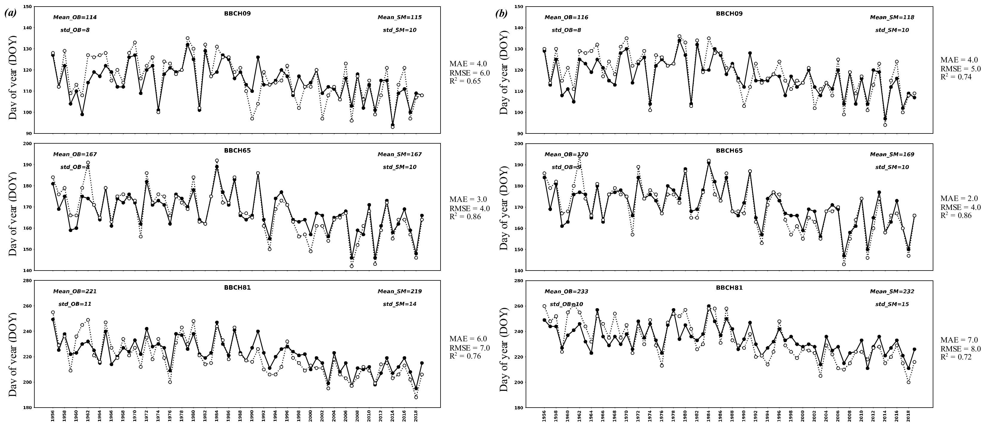
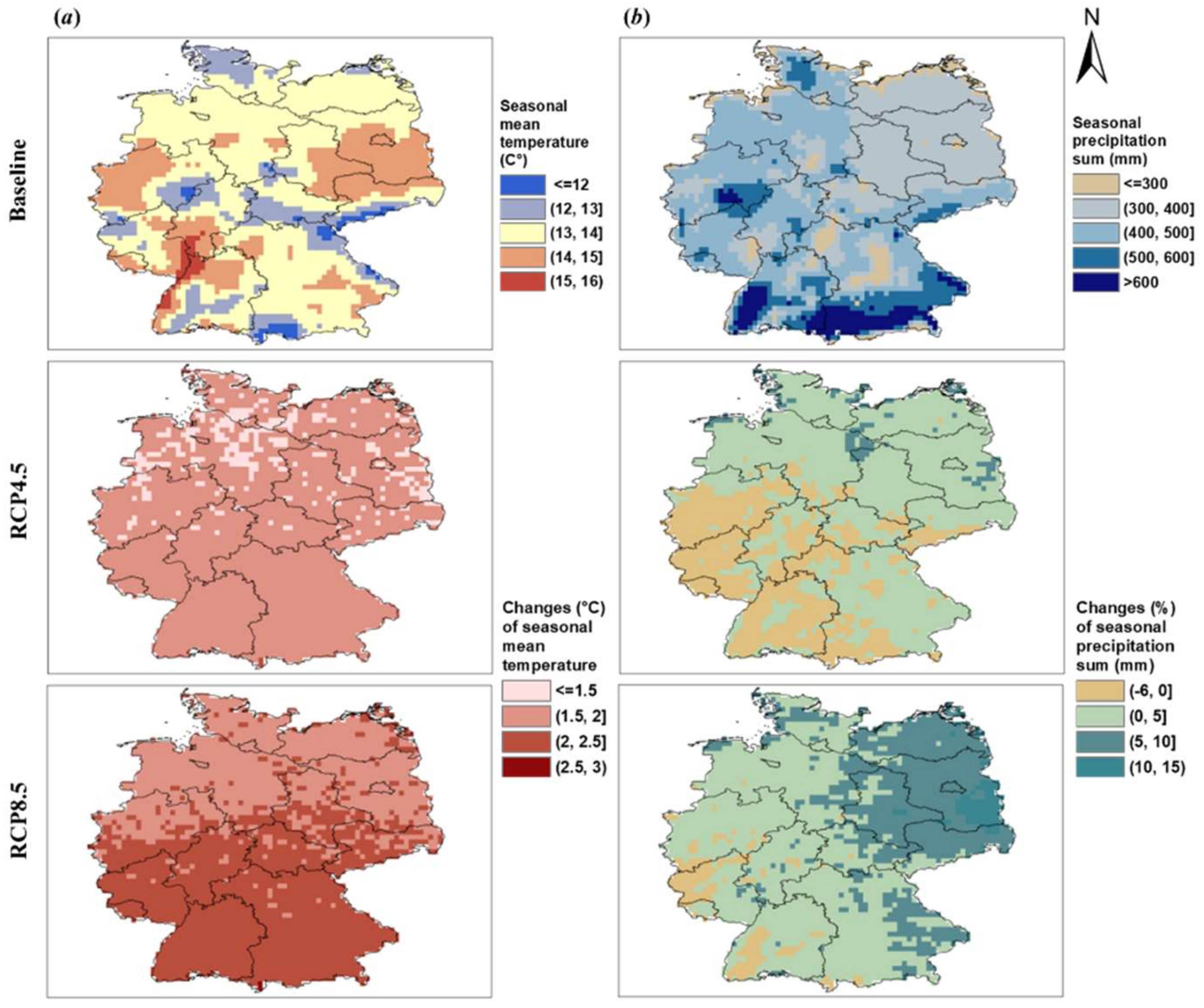
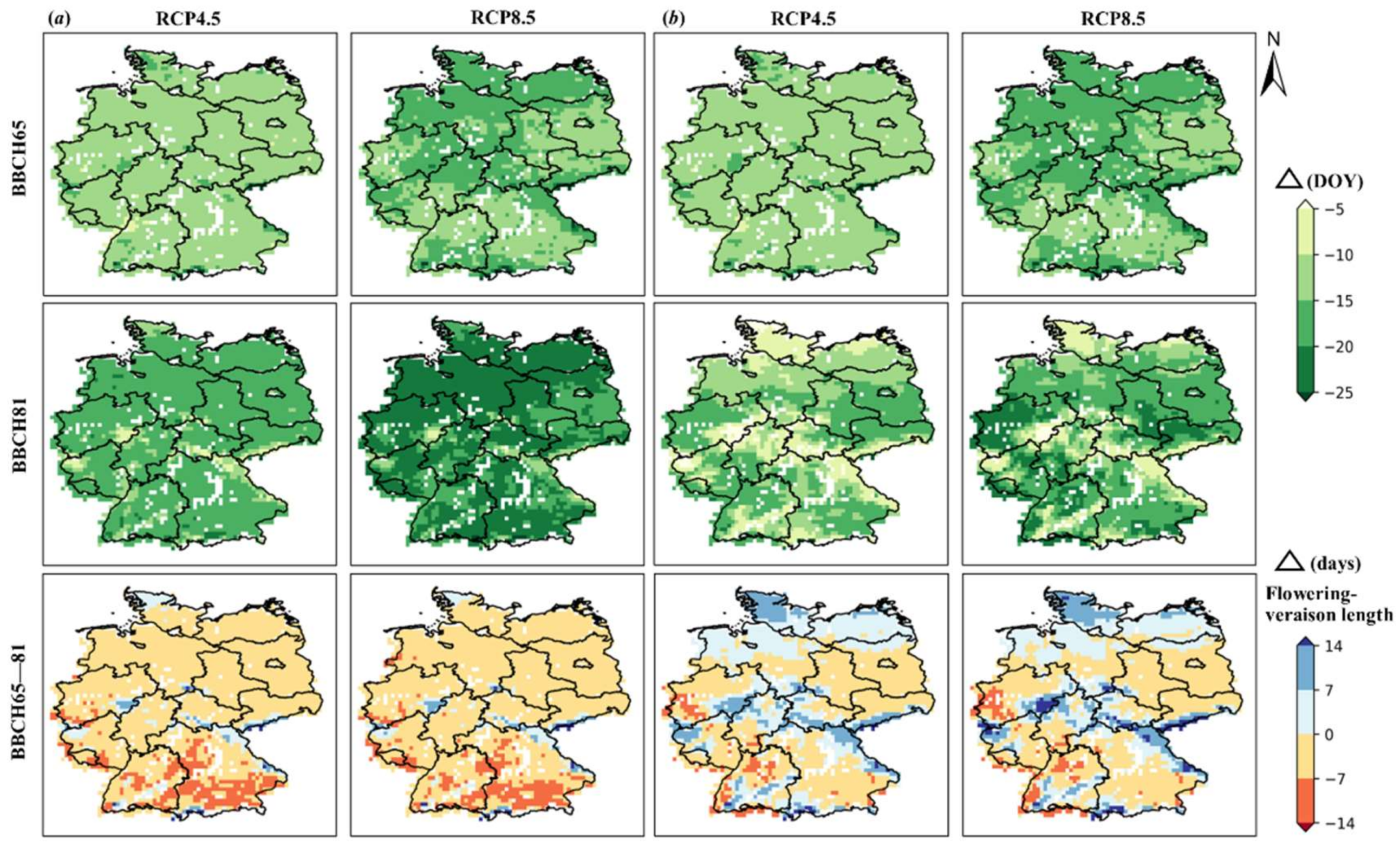

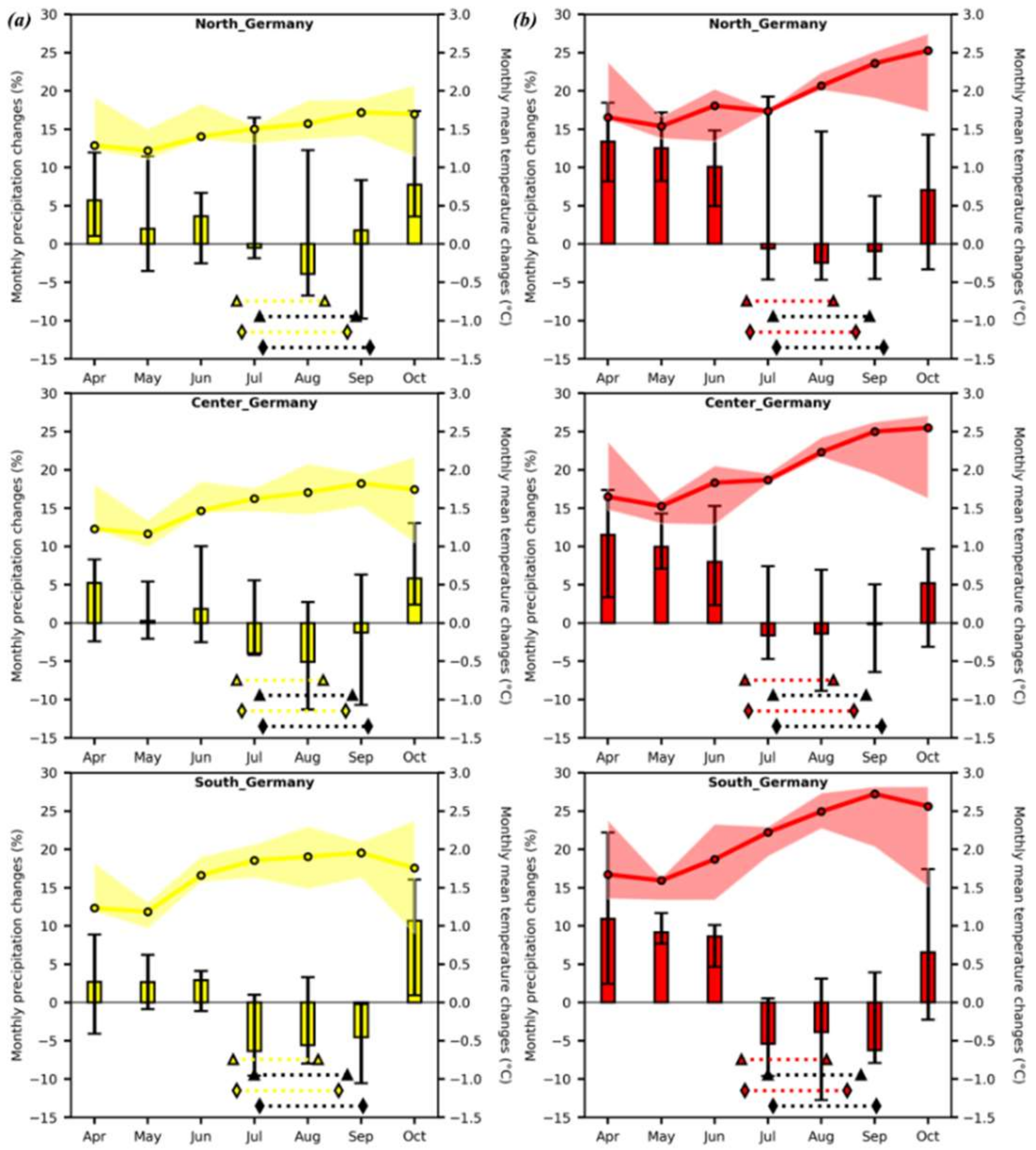
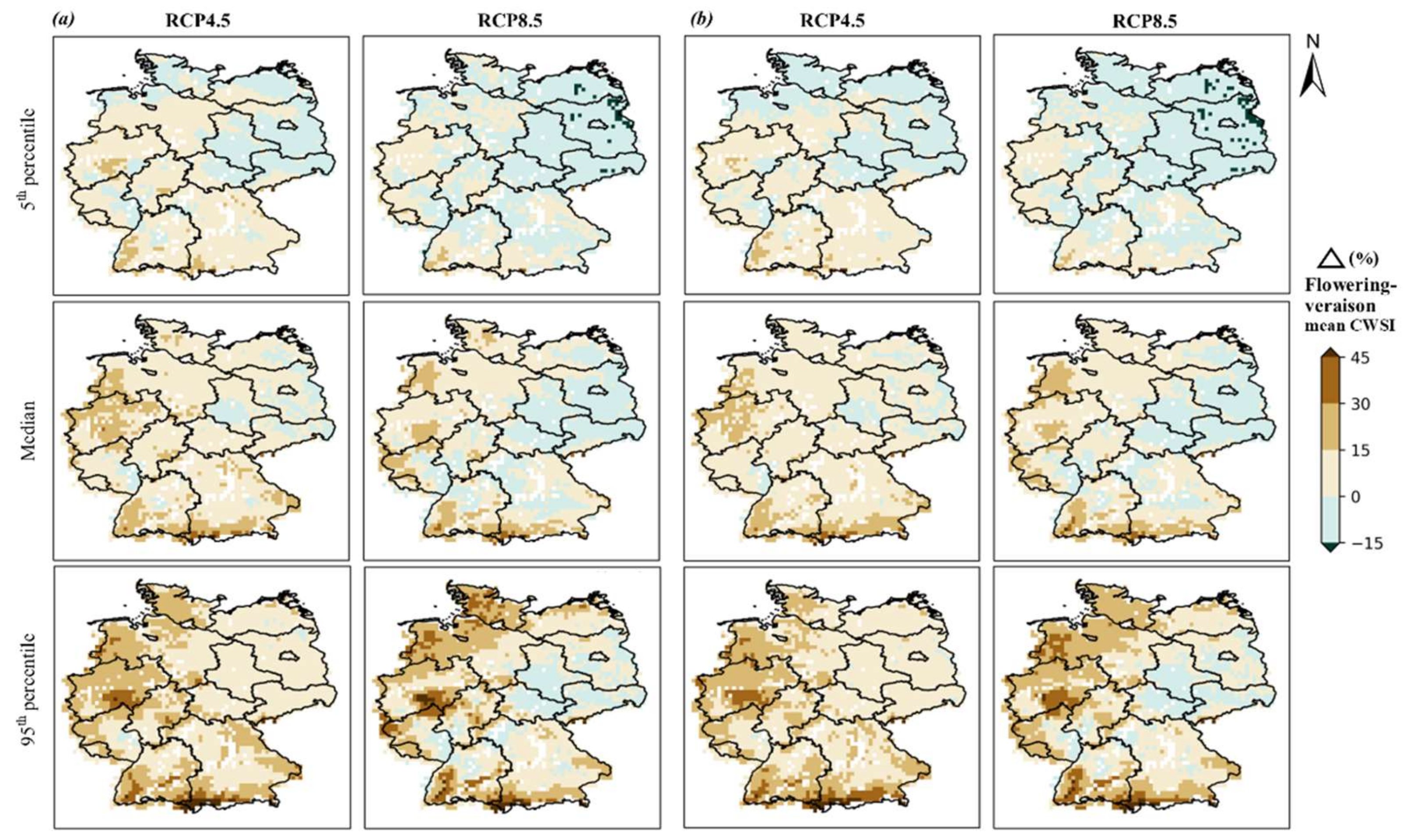
Publisher’s Note: MDPI stays neutral with regard to jurisdictional claims in published maps and institutional affiliations. |
© 2022 by the authors. Licensee MDPI, Basel, Switzerland. This article is an open access article distributed under the terms and conditions of the Creative Commons Attribution (CC BY) license (https://creativecommons.org/licenses/by/4.0/).