Condition Monitoring of Wind Turbine Main Bearing Based on Multivariate Time Series Forecasting

Abstract

Condition monitoring and overheating warnings of the main bearing of large-scale wind turbines (WT) plays an important role in enhancing their dependability and reducing operating and maintenance (O&M) costs. The temperature parameter of the main bearing is the key indicator to characterize the normal or abnormal operating condition. Therefore, forecasting the trend of temperature change is critical for overheating warnings. To achieve forecasting with high accuracy, this paper proposes a novel model for the WT main bearing, named stacked long-short-term memory with multi-layer perceptron (SLSTM-MLP) by utilizing supervisory control and data acquisition (SCADA) data. The model is mainly composed of multiple LSTM cells and a multi-layer perceptron regression layer. By combining condition parameters into a characteristic matrix, SLSTM can mine nonlinear, non-stationary dynamic feature relationships between temperature and its related variables. To evaluate the performance of the SLSTM-MLP model, experimental analysis was carried out from three aspects: different sample capacity sizes, different sampling time segments, and different sampling frequencies. Furthermore, the model’s capability of online fault detection was also carried out by simulation. The results of comparative studies and online fault simulation tests show that the proposed SLSTM-MLP has better performance for temperature forecasting of the main bearing of large-scale WTs.

1. Introduction

Wind energy is the most widely used clean and low-carbon renewable energy with the fastest development. More and more countries have attached great importance to wind turbines, and many wind farms and larger capacity large-scale wind turbines are coming into use. However, because of the harsh natural working environment (especially for offshore large-scale wind turbines) complex and changeable operating condition of large-scale wind turbines (WT), some core components, such as main bearings, frequently fail, resulting in prolonged downtime and increased O&M costs of wind farms [1]. Therefore, in order to enhance component reliability, avoid faults, and reduce O&M cost, it is of vital practical significance to study the operating condition monitoring methods of the core components of large-scale WTs [2].

The main bearing of large-scale WTs, as an important physical component of the WT transmission chain, connects the hub and the generator or the gearbox. According to the European Academy of Wind Energy (EAWE) [3], WT main bearings have been identified as one of the critical components in terms of increasing WT reliability and availability for the transmission system in the wind industry. The WT main bearing is a large component, and its internal structure is complicated. Furthermore, the operating environment of the WT main bearing is very harsh and complex, and the alternating load in the axial and radial directions and strong impact make it prone to failure. According to literature reports, the failure rate of the WT main bearings reaches 15% and 30% [4]. A lot of research has been carried out on monitoring the operating conditions of the WT main bearings [5]. These methods are mainly divided into two categories, i.e., vibration-based analysis methods and temperature-based analysis methods. (1) Vibration-based analysis methods include the following. Natili et al. [6] used the vibration data of the turbine condition monitoring (TCM) to realize multi-scale condition monitoring and fault detection of the WT main bearings. Artigao et al. [7] used the fast Fourier transform method to analyze the frequency domain of the bearing vibration spectrum to identify bearing faults on the drive chain of wind turbines under different loads. Siegel et al. [8] used fast Fourier transform and envelope analysis to analyze the frequency domain of bearing vibration spectrum to identify bearing faults on the drive chain of wind turbines. Peeters et al. [9] proposed a more intelligent automated cepstrum editing procedure (ACEP) for peak automatic selection based on vibration signal parameters to detect bearing faults. Lu et al. [10] proposed an improved auxiliary classifier generative adversarial network (ACGAN) model with data enhancement function for vibration signal parameters, which balanced vibration data of WT main bearing faults and improved the accuracy of fault diagnosis of the WT main bearing. The above works mainly focus on the analysis and modeling of high-frequency vibration data. However, in the actual wind field SCADA system, the collected data are usually low-frequency vibration data, such as 1 s, 1 min, 5 min, 10 min, etc. These methods may not be suitable. In addition, the relationship between field SCADA data parameters is complex, and the existing shallow machine learning methods have limited ability to extract features. Although the deep learning GAN model is adopted in the literature [10], its data also comes from the laboratory rather than the field. Therefore, the analysis and modeling of low-frequency vibration data and multi-parameters are less accurate. (2) Temperature-based analysis methods include the following. Zhang [11] utilized SCADA data to build a neural network model to forecast the temperature of the WT main bearing to diagnose the main bearing failure. Zhao et al. [12] used SCADA data condition parameters, such as the temperature of the WT main bearing, to build a restricted Boltzmann machine-based deep learning model, which can reconstruct the overall WT main bearing conditions to predict the faults of the WT main bearing. Wang et al. [13], based on SCADA data, constructed a deep belief network based on a restricted Boltzmann machine (RBM) to predict the temperature of the WT main bearing and to monitor and detect anomalies of the WT main bearing. Zhao et al. [14] proposed an improved deep belief network based on RBM to reconstruct the normal condition of the WT main bearing and used the reconstruction error to monitor and detect whether the WT main bearing was in an abnormal condition. Yucesan et al. [15] established a deep neural network model based on the fusion of physical information and data-driven parameters such as the main bearing temperature to detect the fatigue and oil degradation of the main bearing. The above studies have examined a variety of methods, from simple neural network structure to complex deep belief models. These studies carried out main bearing condition monitoring, fatigue detection, and oil degradation by reconstructing a vector or predicting a single value. However, some methods do not consider wind speed, parameter selection, and model structure determination in detail, and some temperature prediction models have low accuracy and large error.

In summary, condition monitoring and fault detection of the main bearing of large-scale WTs-based on the WT SCADA system has become a research hotspot [16,17]. The research results of the vibration-based analysis method and temperature-based analysis method described above have deepened the understanding of operating state monitoring, detection, and fault detection of the main bearing of large-scale WTs based on the application of these methods, such as neural network models, support vector machines, deep belief networks, and adversarial learning. However, some of the models above are shallow machine learning models, which have limited ability to comprehensively extract data features from the SCADA dataset. In addition, parameter selection and structure determination for models are not discussed in detail, which limits the application and promotion of models to a certain extent. Some research needs to be further expanded.

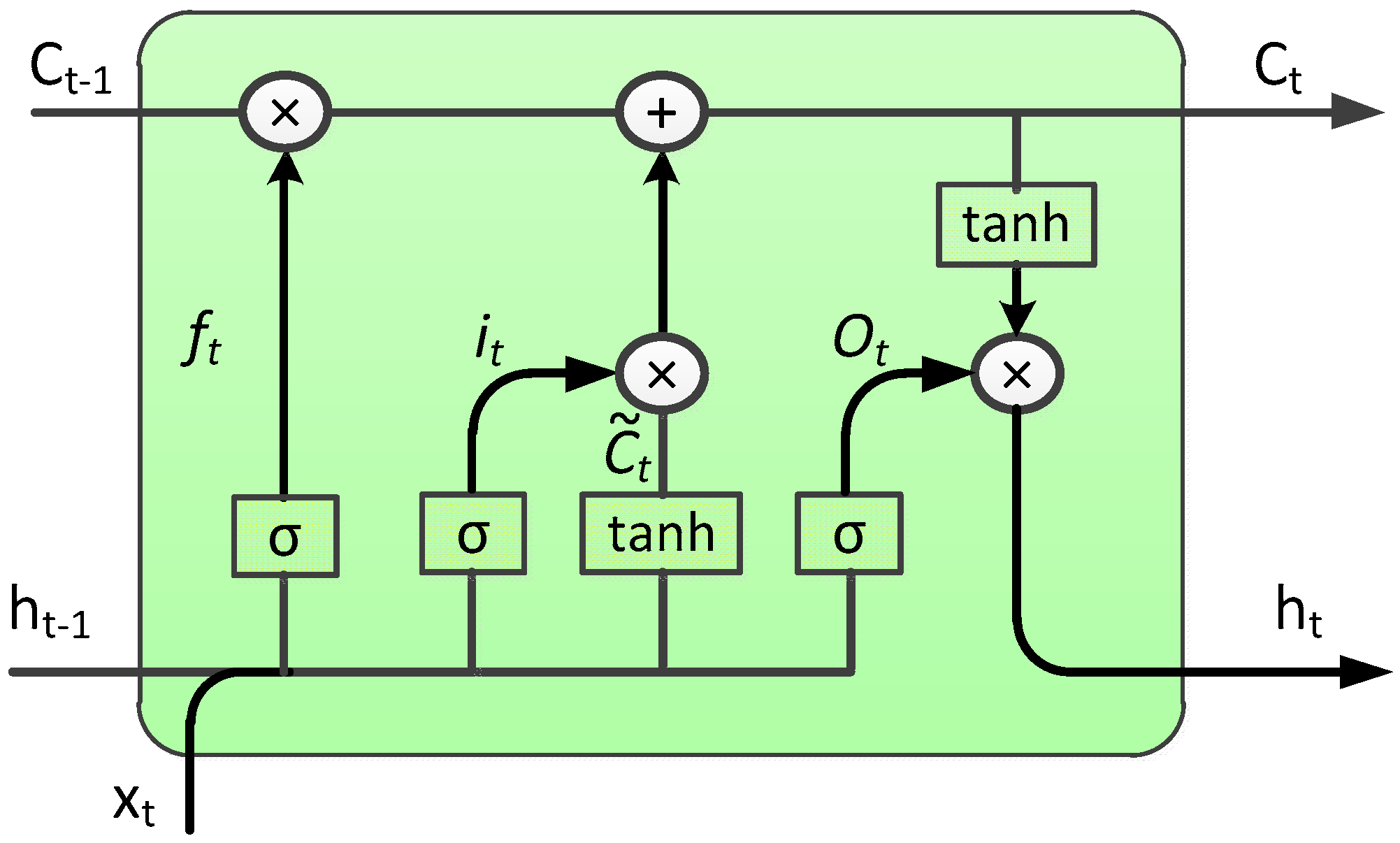
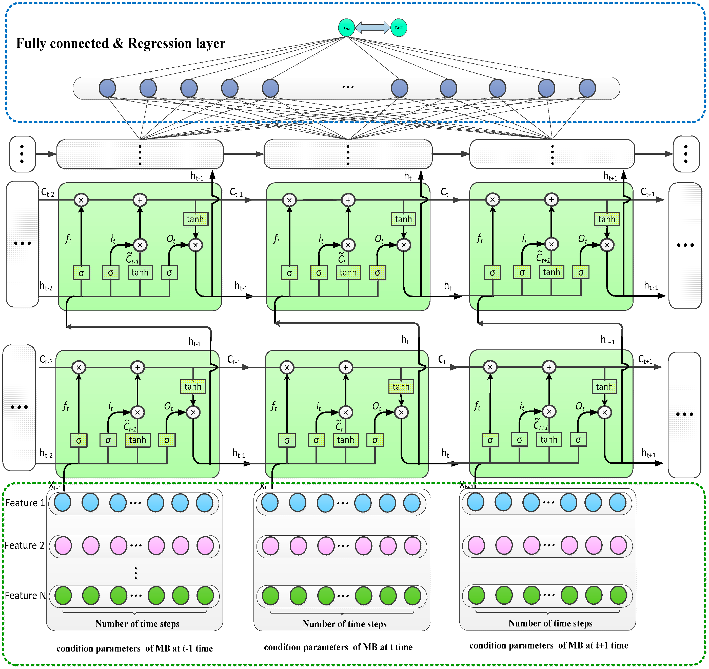
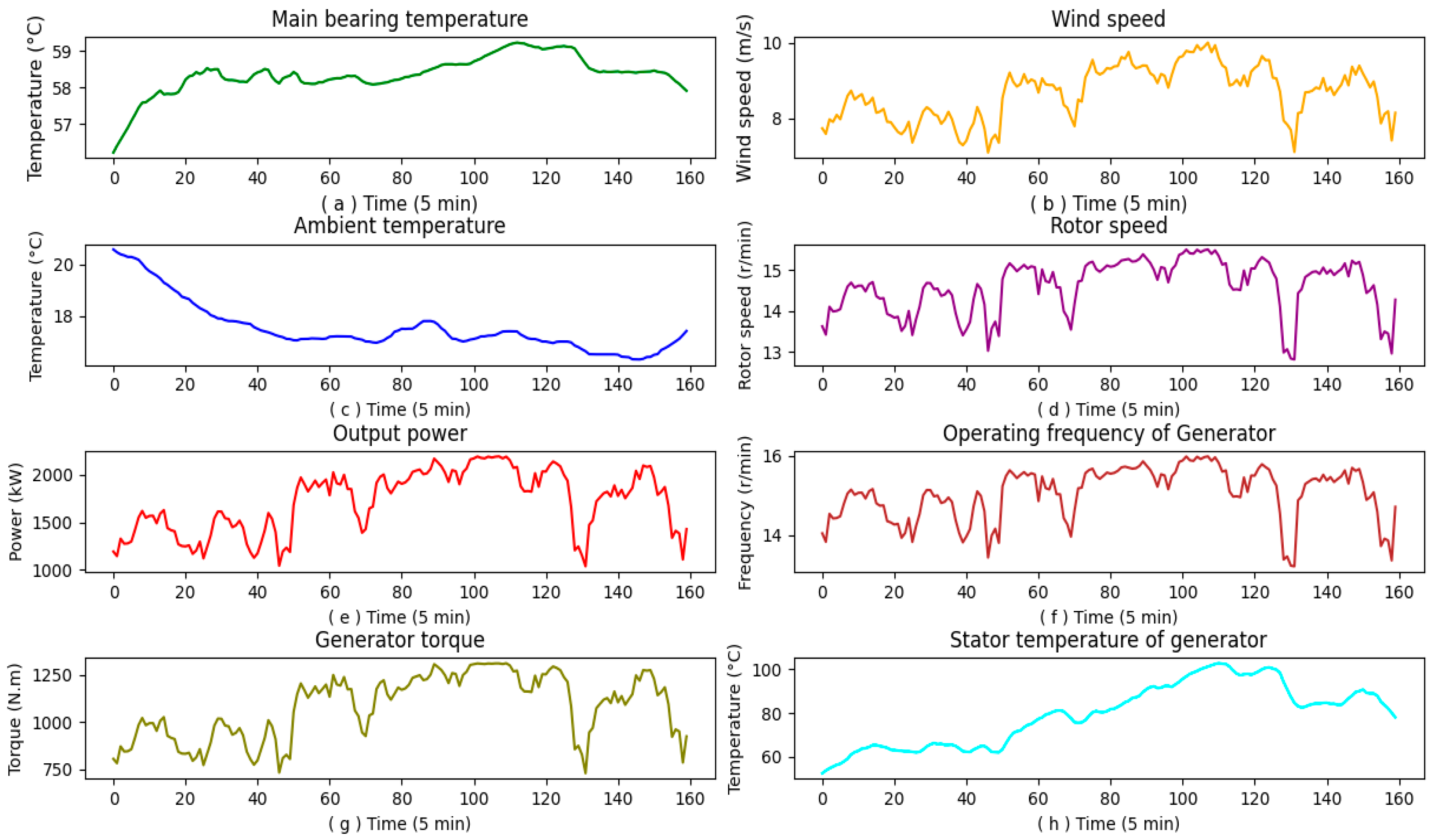
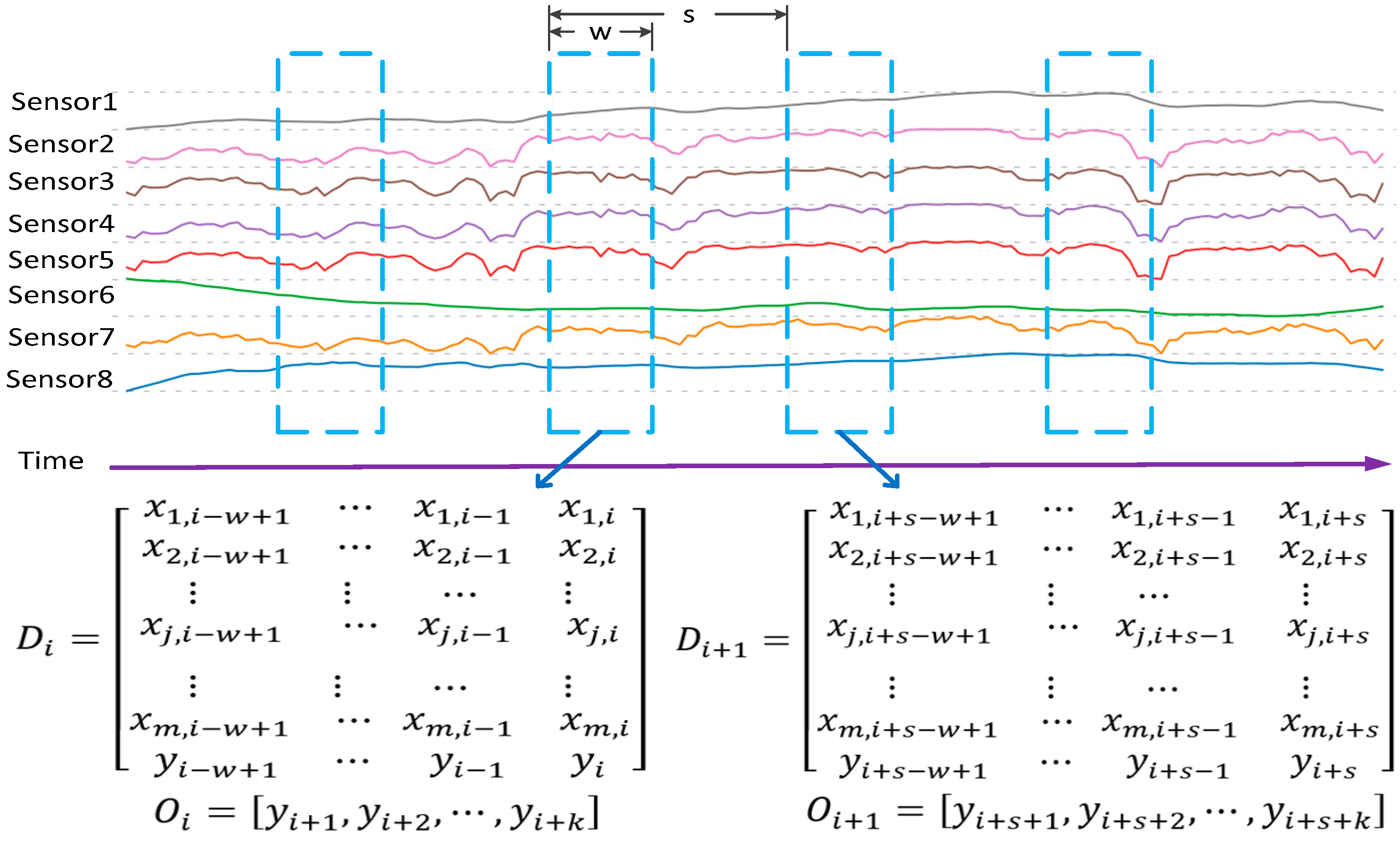
In this paper, we take the main bearing of large-scale direct-driven WTs as the research object to carry out operating condition monitoring and abnormal detection research based on SCADA data from a real wind farm. It is well known that the temperature of the main bearing of large-scale direct-driven WTs is an important parameter to monitor to determine whether the WT main bearing is abnormal. In the long-term monitoring process, temperature time series does not have obvious details of high-frequency mutation, but has certain random characteristics, obvious temporal characteristics, and short-term correlation. The model based on long-short term memory (LSTM) is very suitable for dealing with this situation. LSTM network models have great processing power for solving long-term or short-term time series dependency problems and can be used to automatically learn the temporal dependence structures of complex relationships between the temperature change of the main bearing itself and other related variables. In addition, the LSTM model, its variants, and combination models have been successfully applied in forecasting and classification [18,19,20]. The motivation for this manuscript is to overcome two issues in the existing research: (1) The mining of time series feature information is insufficient in the existing literature research, and temporal characteristics of multivariable parameters are not considered in condition monitoring and anomaly detection. (2) Model structure determination and hyper-parameter selection are not discussed in-depth, and the model has poor reproducibility, which leads to application limitations of the model. Therefore, in this study, we propose a novel deep learning model for temperature forecasting of the main bearing of large-scale direct-driven WTs by using a SCADA dataset from a real wind farm. Taking a single LSTM cell as the basic component, we stack LSTM cells to build a deep model with multiple perceptual regression layers, named stacked long-short term memory with multi-layer perceptron (SLSTM-MLP), to provide robust operating condition monitoring and anomaly detection through multivariate time series datasets. The main contributions of this paper are summarized as follows:

(1)

A novel deep learning network framework SLSTM-MLP is proposed for forecasting the temperature of the main bearing of large-scale direct-driven WTs to mine time-series information of multiple parameter variables and coupling information between parameter variables. In the model, we stack multiple LSTM cells to train for achieving high forecasting accuracy in order to obtain the nonlinear and non-stationary dynamic features relationship between temperature itself and its related parameter variables.

(2)

We conduct extensive experiments utilizing SCADA data to evaluate the performance for the proposed model from different sample capacity sizes, different sampling time segments, and different sampling frequencies. The experimental results show that the SLSTM-MLP model is superior to the other approaches.

(3)

We put forward a framework for online condition monitoring and abnormal detection of WT main bearings and then simulate two different degree faults by adding two cumulative temperature offsets to two associated variables. The simulation results show that the proposed SLSTM-MLP model is effective in the forecasting and monitoring process.

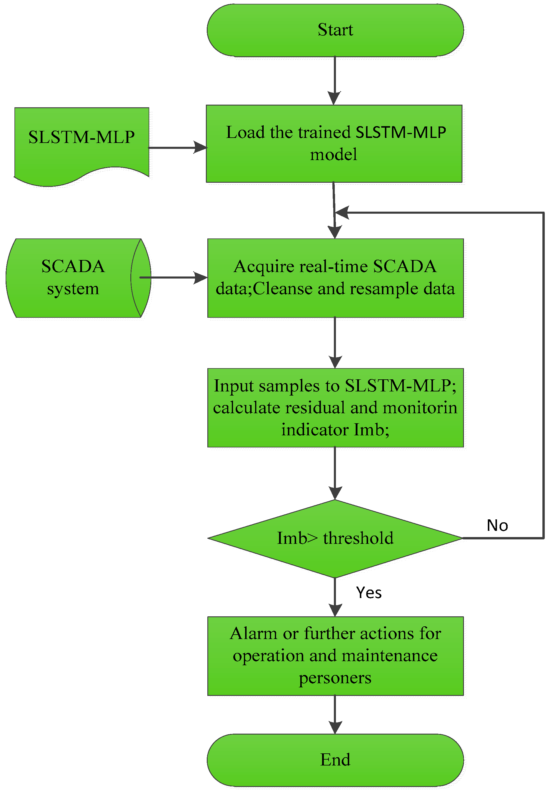
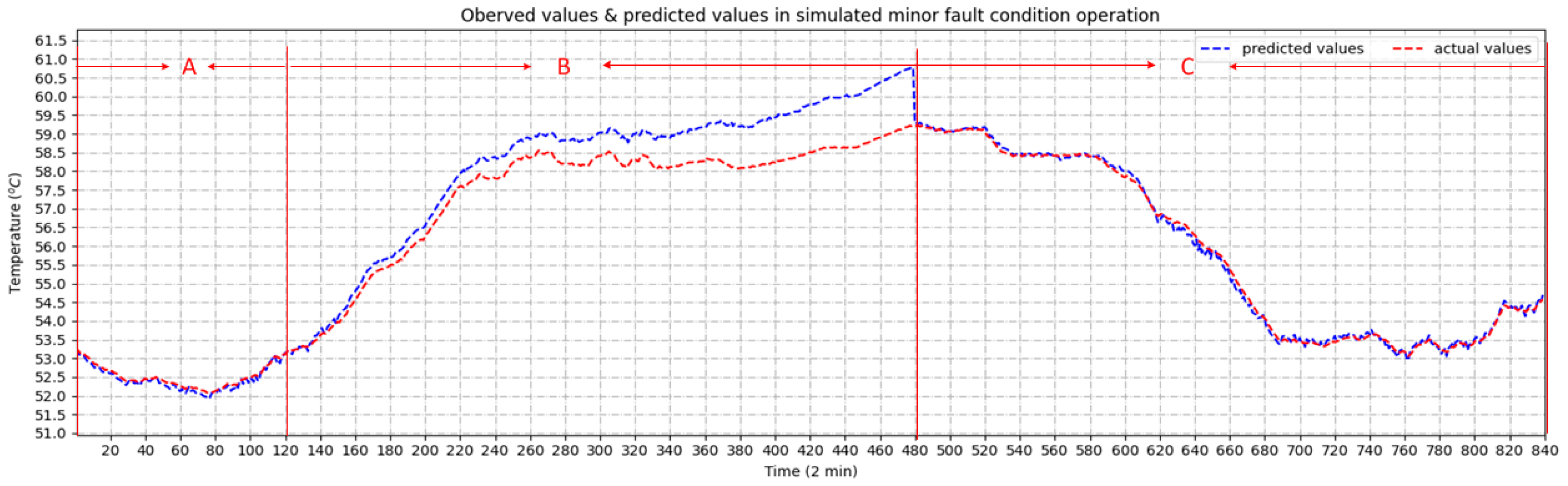
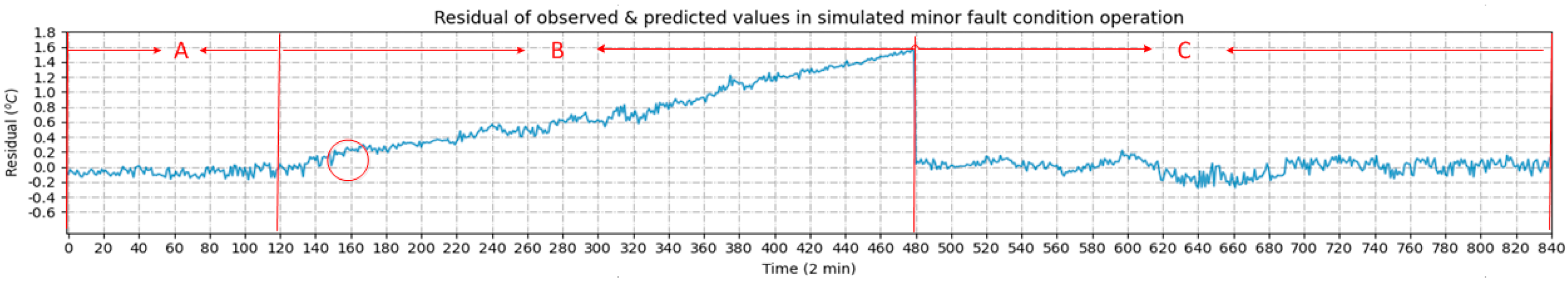
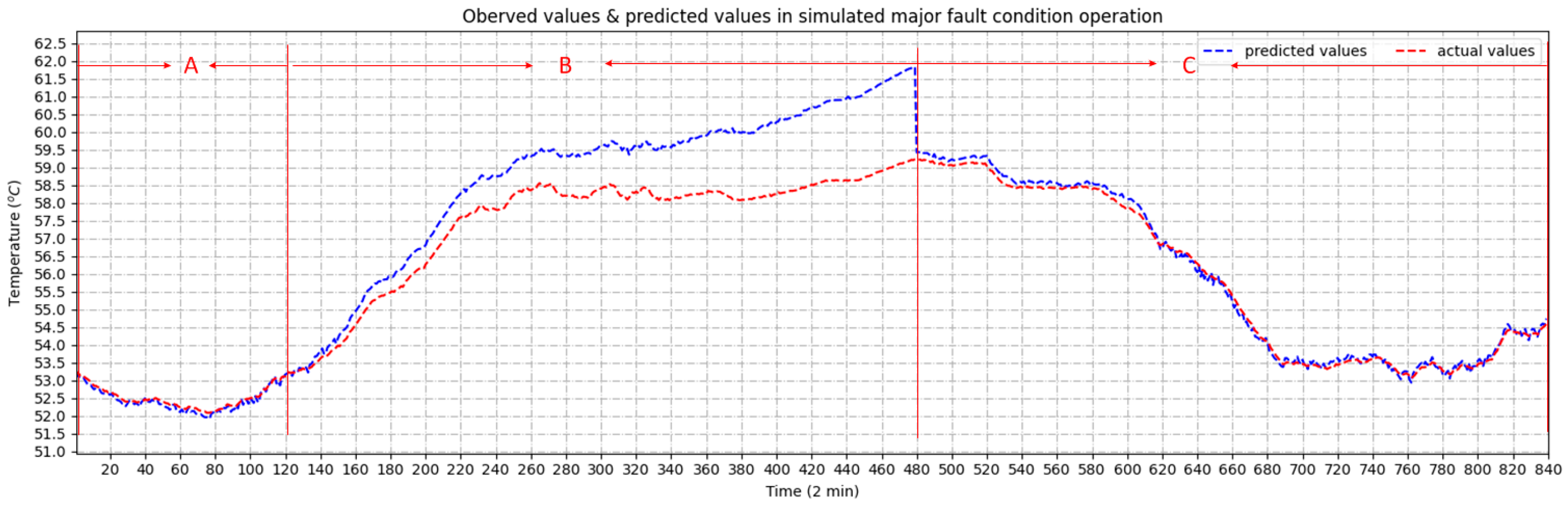
The remainder of this paper is organized as follows. Section 2 presents the proposed SLSTM-MLP model, including the problem definition, the framework, and training algorithm. Section 3 describes the experiment setup, data cleansing and resampling, and model structure determination. Performance comparison with other models is presented in Section 4. The framework for online operating condition monitoring and abnormal detection and fault simulation are presented in Section 5. Finally, conclusions are drawn in Section 6.

2. The Proposed Method of SLSTM-MLP

In this section, we first give the definition of the multivariable time series forecasting problem of the WT main bearing temperature. Then, we introduce some basic theoretical knowledge of LSTM. Then, we put forward a novel deep learning recurrent neural network framework for large-scale WT main bearing temperature forecasting through a multivariable time series modeling method. At last, we introduce the corresponding training algorithm for the proposed SLSTM-MLP model.

2.1. Problem Definition

Temperature time series data of WT main bearing has strong autocorrelation with its historical values and also has a strong correlation with the other related external variables, such as wind speed, output power, rotor speed, ambient temperature, generator stator temperature. Therefore, the temperature time series forecasting problem of WT main bearing is a multivariable time series (MTS) forecasting problem with temperature itself and several other related variables. It is still challenging to effectively model such correlations and then enable accurate condition monitoring. The multivariable time series forecasting problem of the main bearing temperature of WT is described as follows:

$$\left[y_t,y_{t+1},\dots ,y_{t+k-1}\right]=f\left({\mathit{X}}_{t-1},{\mathit{Y}}_{t-1}\right)$$

(1)

where ${\mathit{X}}_{t-1}=\left\{x_{1,t-1},x_{1,t-2},\dots ,x_{1,t-n};x_{2,t-1},x_{2,t-2},\dots ,x_{2,t-n};\dots ;x_{m,t-1},x_{m,t-2},\dots ,x_{m,t-n}\right\}\in R^{m\ast n.}$ represents the historical dataset of the conditional parameter related to the WT main bearing before time interval t, and m is the number of related conditional parameter variables; ${\mathit{Y}}_{t-1}=\left\{y_{t-1},y_{t-2},\dots ,y_{t-n}\right\}\in R^n$ represents historical data backward from the current time interval t; n represents the length of the series; $\left[y_t,y_{t+1},\dots ,y_{t+k-1}\right]\in R^k$ is the forecasted temperature of the WT main bearing at the next k time interval; $f$ is a complicated nonlinear mapping function. We label $\left({\mathit{X}}_{t-1},{\mathit{Y}}_{t-1}\right)$ as ${\mathit{D}}_t$, and $\left[y_t,y_{t+1},\dots ,y_{t+k-1}\right]$ as ${\mathit{O}}_t$ in subsequent analysis.

2.2. LSTM Theoretical Basis

LSTM, a special recursive neural network model, was proposed by Hochreiter and Schmidhuber [21] and is well suited to capture nonlinear and non-stationary dynamic features for time series data sequences. It has been widely used in speech recognition, natural language processing, machine translation, video tagging, and generated image description [22,23,24,25]. A single LSTM cell consists of a cell state, a forgetting gate, an input gate, and an output gate. Its internal structure is shown in Figure 1.

As shown in Figure 1, the ${\mathit{x}}_t$ represents input data vector. The ${\mathit{h}}_{t-1}$ and ${\mathit{h}}_t$ represent the hidden state vector of the cell in the previous time step t-1 and at the current time step, respectively. The ${\mathit{C}}_{t-1}$ and ${\mathit{C}}_t$ represent the cell state at the previous time step and current time step, respectively. The ${\mathit{f}}_t$, ${\mathit{i}}_t$, and ${\mathit{O}}_t$ represent the forget, input, and output gates, respectively; $\sigma$ and $tanh$ represent two kinds of activation functions, namely sigmoid and tanh. Based on the backpropagation through time (BPTT) algorithm, these parameters are updated by the following formulas:

$${\mathit{f}}_t=\sigma \left({\mathit{W}}_f\ast \left[{\mathit{h}}_{t-1},{\mathit{x}}_t\right]+{\mathit{b}}_f\right)$$

(2)

$${\mathit{i}}_t=\sigma \left({\mathit{W}}_i\ast \left[{\mathit{h}}_{t-1},{\mathit{x}}_t\right]+{\mathit{b}}_i\right)$$

(3)

$${\tilde{\mathit{C}}}_t=tanh\left({\mathit{W}}_c\ast \left[{\mathit{h}}_{t-1},{\mathit{x}}_t\right]+{\mathit{b}}_c\right)$$

(4)

$${\mathit{C}}_t={\mathit{f}}_t\ast {\mathit{C}}_{t-1}+{\mathit{i}}_t\ast {\tilde{\mathit{C}}}_t$$

(5)

$${\mathit{O}}_t=\sigma \left({\mathit{W}}_o\ast \left[{\mathit{h}}_{t-1},{\mathit{x}}_t\right]+{\mathit{b}}_o\right)$$

(6)

$${\mathit{h}}_t={\mathit{O}}_t\ast tanh\left({\mathit{C}}_t\right)$$

(7)

where ${\mathit{W}}_f$, ${\mathit{W}}_i$, ${\mathit{W}}_c$, ${\mathit{W}}_o$, ${\mathit{b}}_f$, ${\mathit{b}}_i$, ${\mathit{b}}_c$, and ${\mathit{b}}_o$ represent the corresponding weight coefficient matrixes and bias terms, respectively.

2.3. The Framework of the Proposed Model

To further mine the temporal correlation from the SCADA data related to WT main bearings and achieve forecasting with high accuracy, we developed the framework of the SLSTM-MLP model for WT main bearing temperature forecasting with a multivariable time series modeling method. The framework consisted of four parts: input layer, multi-hidden layers, fully connected layer, and regression output layer. The framework of the SLSTM-MLP model is shown in Figure 2.

The input layer is an input matrix $\mathit{X}$ with multivariate time series, which is defined as a tensor of shape (S, M) format, where S represents the number of time steps, and M represents the number of variables. In our experiment, M was set to 8, and S needs to be verified by incrementing one by one starting from integer 1. The multi-hidden layer includes multiple LSTM units. These LSTM units take the output of the ith hidden layer as the input of the (i + 1) hidden layer and are stacked to form a multi-layer network to learn the nonlinear and non-stationary feature representations of the original data. Each hidden layer extracts different levels of feature representation at different time steps until finally, the last layer provides the output. The benefit of the stacked LSTM architecture is that the additional LSTM hidden layer can extract the learned data characteristic representation of the previously hidden layer to form a higher level of abstraction feature extraction. Practice has shown that the depth of the network is as important as the number of cells. The fully connected layer accepts the output vector of the last LSTM model, whose dimension is equal to the number of neurons in the hidden layer, and it completes the dimension transformation. The output layer can be a classifier or a regressor, and in this article, we use a regressor for the WT main bearing temperature forecasting.

2.4. Training Algorithm for the SLSTM-MLP Model

Now, we present the corresponding training algorithm for the SLSTM-MLP model according to the framework in Figure 2. The major steps of the SLSTM-MLP model algorithm can be described as: (a) collecting the normal historical SCADA data from 2 M direct-driven WT; (b) executing the data cleansing and resampling; (c) selecting parameter variables; (d) constructing training and testing dataset; (e) building the SLSTM-MLP model; and (f) training and validating the SLSTM-MLP model. The algorithm pseudocode is outlined in Algorithm 1.

Algorithm 1: Training the SSAE-MLP Model
Input:$D=\left\{\left(D_1,O_1\right),\dots ,\left(D_i, O_i\right),\dots \right\}, D_i\in R^{\left(m+1\right)\ast w},O_i\in R^k$
Output: The optimal SLSTM-MLP model (*.h5)
1:	Read normal historical SCADA data from csv files;
2:	Clean and resample data;
3:	Select related conditional parameter variables;
	//construct training dataset and verify dataset
4:	$D=\varnothing , TD=\varnothing , VD=\varnothing$
5:	for i in range (1, n-w) do: // set the sliding step is 1
6:	$D=D{\displaystyle \cup }{D}_i$
7:	end for
8:	According to the ratio of 80% and 20%, split the $D$ to generate $TD, VD$
	//train SLSTM-MLP model
9:	Assign maximum values to these parameters: hidden layers ${\mathrm{n}}_{\mathrm{l}}$, units ${\mathrm{s}}_{\mathrm{l}}$,
	iterations $e$, and set the range of learning rate $l_r$, batch size batch;
10:	Initialize parameters;
11:	while i <= e:
12:	Train the model using training data in batches;
13:	Use adam or BPTT algorithms to optimize the model;
14:	Verify the model using verify dataset;
15:	Reserve the optimum parameters;
16:	end while
17:	Return The optimal SLSTM-MLP model (*.h5);

3. Experiment Setup and Model Determination

In this section, we first explore the characteristics of the WT SCADA dataset. Then, we descript experimental setup details, including the selection of condition parameters, data cleansing and resampling, and training dataset construction. At last, we analyze the structure determination of the proposed model in detail. The experiments are conducted on the server cluster, and the assigned virtual machine (VM) has a dual-core central processing unit (CPU) configured by a 2.2 GHz Inten (R) E 7-8860 processor with 32 GB RAM, using Python 3.6 software package and Keras API under Windows 10 pro with 64-bit operating system to development.

3.1. Data Description

In this study, our research focuses on a 2 MW direct-driven WT with cut-in, rated, and cut-out wind speeds of 3, 11, and 25 m/s, located at Lu Hejin wind farm in Chenzhou, southern China. We collected the dataset from the WT SCADA system with a 1 Hz sampling frequency. The dataset records 155 conditional parameters for each WT, and all data are stored in 10 min CSV files.

Table 1. Partial raw WT data from SCADA system.

No.	TIME (hh: mm: ss)	WS(m/s)	RS (rpm)	HT (°)	MT (°)	GST (°)	…	OP (kW)
1	00:17:31	7.0	11.45	39.4	50.3	49.1	…	687
2	00:17:32	6.7	11.42	39.4	50.3	49.1	…	691
3	00:17:33	6.7	11.40	39.4	50.3	49.1	…	691
4	00:17:36	null	null	null	null	null	…	null
5	00:17:37	0	0	0	0	0	…	0
6	00:17:38	7.5	11.44	39.4	50.2	49.1		697
…	…	…	…	…	…	…	…	…

Notation: TIME, record time; WS, wind speed; RS, rotor speed; HT, hub temperature; MT, main bearing temperature; GST, generator stator temperature; OP, output power.

lists a small portion of the raw data with some specified attribute fields from the SCADA systems.

3.2. Condition Parameters Selection

The collected SCADA dataset from direct-driven WT involves many types of operating condition parameters, such as rote speed, wind speed, voltage, current, temperature, output power, etc. These condition parameters can be used to analyze and evaluate the operating and health conditions of wind turbines. In this paper, we study the main bearing of large-scale direct-driven WTs through temperature indicator variation trends. Based on our previous research, we chose these parameters through correlation analysis and physical information redundancy parameter elimination method. These parameters include wind speed, output power, rotor speed, generator torque, generator stator temperature, generator operating frequency, and environmental temperature, which are shown in

Table 2. Selected operating condition parameters variables of direct-driven WT.

No.	Parameter Variable	Description	Units	Abbr
1	Wind speed	Wind speed with one second	m/s	WS
2	Rotor speed	Hub rotation speed	r/min	RS
3	Output power	Generator output power	kW	OP
4	Generator stator temperature	Mean of six temperature sensors	°C	GST
5	Ambient temperature	Temperature outside nacelle	°C	AT
6	Operating frequency	Generator operating frequency	r/min	GOF
7	Torque	Rotational torque of generator	N.m	GT
8	Main bearing temperature	Mean of two temperature sensors	°C	MBT

[26].

3.3. Data Cleansing and Resampling

In the process of WT SCADA data transmission and storage, some unstable factors, such as control system failure, sensor malfunction, transmission cable problems, etc. lead to null values, outliers, and other invalid data in the WT SCADA dataset, as seen in lines 4 and 5 in Table 1. In order to obtain high-quality data and ensure high precision of subsequent modeling results, data cleaning is needed. In other words, some downtime data, packet loss data, negative data, and null data were deleted in this study. At the same time, we also resampled the data samples according to the practices of existing studies [27,28,29,30]. The detailed calculation method for data cleansing and data resampling is shown in Equation (8) and in our previous study [26].

$$\{\begin{array}{cc}\begin{array}{c}delete{x}_i,\\ x_i=x_{i+1}or{x}_{i-1,}\end{array}& \begin{array}{c}for{x}_i\in haultdata\\ for{x}_i\in packetlossdata\end{array}\\ \begin{array}{c}{x}_i=0,\\ x_i=\frac{1}{2}\left(x_{i-1}+x_{i+1}\right)\end{array}& \begin{array}{c}for{x}_i<0or{x}_{i}isnull\\ \begin{array}{c}for{x}_i\ge 2x_{i-1}and{x}_i\ge 2x_{i+1}or\\ for{x}_i\le x_{i-1}/2and{x}_i\le x_{i+1}/2\end{array}\end{array}\\ \overline{x}=\frac{1}{n}{\displaystyle \sum }_{i=1}^n{x}_i,& others\end{array}$$

(8)

After the collected SCADA data was cleaned and resampled, a partial time series diagram of eight condition parameter variables is shown in Figure 3.

In Figure 3, the wind speed fluctuates greatly, and the three temperature parameters show nonlinear and gradual variation trends. With the increasing wind speed, hub speed, generator torque, and output power also increased correspondingly, and the correlation coefficients between wind speed and hub speed, generator torque, and generator output power were 0.9132, 0.9657, and 0.9718, respectively. With the increase of wind speed, stator temperature and main bearing temperature kept a slowly rising trend, and the correlation coefficients between wind speed and generator stator temperature and main bearing temperature were 0.7303 and 0.4439, respectively. The abrupt trend of wind speed showed a weakening characteristic in the condition parameters of a large inertia system and became weaker in the temperature parameters trend. The current value of condition parameters is related to the value of a previous period of time. There is a complex inherent correlation and time dependence relationship among the eight condition parameter variables. The correlation coefficient values of these condition parameters are shown in

Table 3. Correlation coefficient of condition parameter variables.

No.	MBT	WS	AT	RS	OP	GOF	GT	GST
MBT	1.0000	0.4439	−0.7014	0.3286	0.5037	0.3288	0.5271	0.7872
WS	0.4439	1.0000	−0.3285	0.9131	0.9718	0.9131	0.9657	0.7303
AT	−0.7014	−0.3285	1.0000	−0.2625	−0.4324	−0.2629	−0.4596	−0.6334
RS	0.3286	0.9131	−0.2625	1.0000	0.9311	1.0000	0.9013	0.5194
OP	0.5037	0.9718	−0.4324	0.9311	1.0000	0.9313	0.9966	0.7464
GOF	0.3288	0.9131	−0.2629	1.0000	0.9313	1.0000	0.9015	0.5196
GT	0.5271	0.9657	−0.4596	0.9013	0.9966	0.9015	1.0000	0.7776
GST	0.7872	0.7303	−0.6334	0.5194	0.7464	0.5196	0.7776	1.0000

.

3.4. Dataset Construction

The current value of the eight condition parameter variables is affected by its previous values, and these values show obvious temporal characteristics. In order to explore the complex internal relationship and temporal characteristic relationship between variables, we used the sliding window method to process the raw data and generate an input dataset and output dataset. The specific construction process is shown in Figure 4.

From Figure 4, w is the width of the sliding window, s is the length of the sliding step, and $D_i$ and $D_{i+1}$ are taken as input feature vectors, which represent the relevant conditional parameter variables before time interval i and historical data backward of the main bearing temperature from the current time interval i.$O_i$ and $O_{i+1}$ are output feature vectors, which represent the main bearing temperature values at the next n steps.

3.5. Forecasting Evaluation Metrics

Three evaluation metrics were used to evaluate the forecasting results, namely MAE (mean absolute error), MSE (mean square error), and $R^2$ (R-squared). Their expressions can be listed as follows:

$$MAE=\frac{1}{N}{\displaystyle \sum }_{i=1}^N\left|y_{pre,i}^{\prime }-y_{act,i}\right|$$

(9)

$$MSE=\frac{1}{N}{\displaystyle \sum }_{i=1}^N{(y_{pre,i}^{\prime }-y_{act,i})}^2$$

(10)

$$R^2={\displaystyle \sum }_{i=1}^N{(y_{pre,i}^{\prime }-{\overline{y}}_{act})}^2/{\displaystyle \sum }_{i=1}^N{\left(y_{act,i}-{\overline{y}}_{act}\right)}^2$$

(11)

where $y_{pre,i}^{\prime }$ represents the forecasted value at time interval i; $y_{act,i}$ represents the observed value at time interval i; ${\overline{y}}_{act}$ represents the average of the active value; $N$ represents the number of samples. The smaller the MAE and MSE, the higher the forecasting accuracy will be. $R^2$ is the fitting goodness of the regression model. The closer the value is to 1, the better the model fits the observed value and vice versa.

3.6. Structure Determination of the SLSTM-MLP

In the training process of the SLSTM-MLP, there are several hyperparameters that need to be determined, namely time step, batch size, features, units, learning rate, and dropout. (1) Time step: sequence length (the lagged length of the associated variable in the time dimension). This parameter determines how many historical data are used for each parameter variable to forecast. We should first understand from the mechanism of heat transfer what length is reasonable to choose. (2) Features: the number of variables (the feature dimensions), which is to say the dimension of each sample, these features are interpreted by a vector with multiple related variables served as input features for the model. The dimensions of the input data are equal to the number of features multiplied by the time step. (3) Units: the number of hidden neurons in a single LSTM unit, which is used to remember and store past states; that is, the size of the cell. Cells are parallel, share weights for a given time step, and process input data simultaneously, which determines the output dimension of an LSTM. The unit size usually varies from dozens to hundreds and is usually an integer multiple. (4) Batch size: the number of samples that are input into the neural network training at one time to complete weight parameter calculations and update. The larger the value, the more stable the gradient will be when the model is trained. There are two extreme cases, one is to feed all the samples at once, which is the traditional gradient descent method, and the other is to feed only one sample at a time, which is the stochastic gradient descent method. The convergence rate of the former method is slower than that of the latter. Practice shows that the training of small-batch samples is optimal and usually set as a power of 2, such as 8, 16, 32, 64, and 128. (5) Learning rate: how fast the model can converge to the optimal value. The smaller the learning rate, the slower the gradient descent speed of the loss function, the longer the convergence time of the algorithm, and vice versa. The learning rate can be set as 0.1, 0.01, 0.001, and 0.0001. (6) Dropout: regularization method to prevent overfitting by deleting a proportion of hidden neurons; usually ranges from 10%, 20%, 30%, 40%, and 50%.

Parameter tuning is an important task in machine learning modeling. For these hyperparameter selections, there are two generic approaches, grid search, and randomized search. In this study, we used the grid search method to obtain the optimal parameters. For the input layer, we select eight parameters as input vectors (details are given in Section 3.2), and the other hyperparameter set is shown in

Table 4. Hyperparameters for the SLSTM-MLP model.

No.	Hyperparameters	Value Range	No.	Hyperparameters	Value Range
1	Time step	[1, 2, 3]	5	Learning rate	[0.1, 0.01, 0.001]
2	Features	8	6	Dropout	[0.1, 0.2, 0.3]
3	Units	[5, 10, 15, …, 200]	7	Epoch	100
4	Batch size	[8, 16, 31]	8	optimizers	Adam

.

Since there is a certain randomness in the training process of deep learning models with different structures, i.e., the same input for the same structural model will yield different results and also show some random instability. Therefore, by executing each structural model multiple times and by analyzing the statistical characteristics of these experimental results, we will get the best one for temperature forecasting of the WT main bearing. In this study, we first defined 9 basic structures through repeated experiments, namely Model 1, Model 2, and Model 3, respectively, represent the single-layer LSTM Model with 1 to 3 timesteps; Model 4, Model 5, and Model 6, respectively, represent the two-layer LSTM Model with 1 to 3 timesteps; Model 7, Model 8, and Model 9 represent three-layer LSTM models with 1 to 3 timesteps, respectively. Then, we ran each structural model ten times by using the grid search method, and the experimental results of the indicator MAE and R² values are shown in Figure 5 and Figure 6, respectively. To evaluate the performance and stability of these models, we considered the mean and variance of each structural model as the evaluation basis. In addition to considering the mean as small as possible, we further considered variance as small as possible because the mean is susceptible to the influence of extreme values (maximum and minimum values), while variance describes the degree of dispersion between the data value and the mean, which better reflects the stability of the model. From Figure 5, with the increase of the number of layers, the median values of all models show a fluctuating trend of decreasing first and then increasing, and the overall trend shows a fluctuating rising pattern. Figure 6 shows a similar reverse trend, i.e., the fitting degree R² of the regression models shows a fluctuating trend of increasing first and then decreasing, and the overall trend shows a fluctuating decreasing pattern. Figure 5 and

Table 5. Performance indexes of different SLSTM-MLP models.

Model	Testing Datasets
	MAE	MSE	R2
Mode 1	0.064433 ± 0.007577	0.00689 ± 0.001184	0.987706 ± 0.002110
Model 2	0.055311 ± 0.007579	0.005166 ± 0.001053	0.990768 ± 0.001882
Model 3	0.065707 ± 0.006600	0.007294 ± 0.001333	0.986966 ± 0.002382
Model 4	0.059168 ± 0.004467	0.005957 ± 0.000969	0.989383 ± 0.001727
Model 5	0.065263 ± 0.006892	0.006824 ± 0.000929	0.987806 ± 0.001660
Model 6	0.074838 ± 0.006858	0.008535 ± 0.001388	0.983134 ± 0.002481
Model 7	0.068202 ± 0.009132	0.007700 ± 0.001635	0.986276 ± 0.002914
Model 8	0.073384 ± 0.005767	0.008504 ± 0.000551	0.984804 ± 0.000984
Model 9	0.076044 ± 0.006411	0.009438 ± 0.001342	0.983134 ± 0.002399

show that, according to the mean, Model 2 performed best, followed by Model 4. Although the mean value of Model 2 was 6.52% lower than that of Model 4, its variance was 69.67% higher than that of Model 4, and its fitting degree R² was 8.24% lower than that of Model 4; furthermore, Model 4 had no extreme outliers while Model 2 had two extreme outliers. Therefore, we chose Model 4 as the final forecasting model for WT main bearing temperature forecasting.

4. Performance Comparison

To evaluate the performance of the SLSTM-MLP model, several rival models were used, such as RNN, GRU, and LSTM, from three aspects: different sample capacity sizes, different sampling time segments, and different sampling frequencies.

4.1. Different Sample Capacity Size

Sample capacity size represents the necessary number of samples in the process of sampling investigation, which affects the accuracy and confidence value to a certain extent. Usually, we choose more than 30 samples, and in this study, we chose 60 and 120 as the research points, respectively. We selected the SCADA experimental data from the objective WT, and some wind speed data are shown in Figure 7.

From Figure 7, the curve represents new time series data of wind speed. We took point 92 as the starting point and 60 and 120 samples forward to form two datasets, named Group A and Group B. The standard deviation of Group B was 64.2% higher than that of Group A, the xmax-xmin value of Group B was 1.5 times that of Group A, and the average wind speed value of Group B was 1.14 times that of Group A. It could be said that time series Group A and Group B represent two completely different wind conditions in a sense. In the following subsections, we explore the performance of the proposed SLSTM-MLP model under two different sample capacity sizes and also compare it with other advanced forecasting models, such as RNN, GRU, and LSTM.

In order to keep the consistency and fairness of the hyper-parameter tuning of the rival models to be compared, we refer to the hyper-parameter tuning method of structure determination for the proposed model and also used grid search methods to conduct hyperparameter tuning for all rival models (RNN, GRU, and LSTM) to find their respective optimal models to predict the WT main bearing temperature. Each rival model was executed 10 times for selecting the optimal structure in the same parameter search range as the proposed SLSTM-MLP model, and the statistics results of multiple execution programs are shown in Figure 8 and Figure 9. As shown in Figure 8 and Figure 9, all rival models showed lower forecasting errors and higher fitting degrees on the same dataset. The best-performing model was the LSTM model, followed by the GRU model, and the least performing model was the RNN model. Specifically, the average MAEs of RNN, GRU, and LSTM were 0.78153, 0.077327, and 0.064433, respectively, and their standard deviations were all lower than 0.023. The average fitting degrees of RNN, GRU, and LSTM were 0.98346, 0.982952, and 0.987706, respectively, and their standard deviations were all less than 0.0045.

Based on the optimal fitting degree and the deviation degree from the median of the forecasting error value as the judgment criteria for selecting the best model, we chose the optimal models among the three rival models to make forecasting under two different sample capacity sizes. The forecasting results of four competitive models are shown in

Table 6. Performance indexes of different models under Group A dataset.

Model	Group A Dataset
	MAE	MSE	R2
RNN	0.063578	0.006382	0.825424
GRU	0.095320	0.013639	0.626888
LSTM	0.066969	0.008633	0.763823
SLSTM-MLP	0.053779	0.004349	0.881015

and

Table 7. Performance indexes of different models under Group B dataset.

Model	Group B Dataset
	MAE	MSE	R2
RNN	0.087615	0.009981	0.971486
GRU	0.058759	0.006037	0.982650
LSTM	0.060581	0.006630	0.981058
SLSTM-MLP	0.059514	0.005353	0.984708

.

In the Group A dataset, as shown in Table 6, the proposed SLSTM-MLP model showed the best performance, followed by the RNN model, and the GRU model showed the worst performance. The interesting thing is that the stacked LSTM model performed better than the single-layer LSTM model. In detail, the MAE value of the proposed model fell by about 15.41%, 43.58%, and 19.7% compared with RNN, GRU, and LSTM, respectively. The MSE value of the proposed model fell by about 31.86%, 68.11%, and 49.62% compared with RNN, GRU, and LSTM, respectively. The fitting degree of the proposed model increased by 6.73%, 40.54%, and 15.34% compared with RNN, GRU, and LSTM, respectively. The detailed forecasting results of all comparative models are presented in Figure 10, and the corresponding forecasting residuals are shown in Figure 11. The predicted values deviate a little from the observed value, especially around the 4th and 25th time points.

In the Group B dataset, as shown in Table 7, the proposed SLSTM-MLP model showed the best performance, followed by the GRU and LSTM model. Meanwhile, the RNN model showed the worst performance. In detail, the MAE of the proposed model fell by about 32.07%, -1.29%, and 1.76% compared with RNN, GRU, and LSTM, respectively. The MSE of the proposed model fell by about 46.37%, 11.33%, and 19.26% compared with RNN, GRU, and LSTM, respectively. The fitting degree of the proposed model increased by about 1.34%, 0.21%, and 0.37% compared with RNN, GRU, and LSTM, respectively. The detailed forecasting results of all comparative models are presented in Figure 12, and the corresponding forecasting residuals are shown in Figure 13.

4.2. Different Sampling Time Segments

In this section, we randomly selected another dataset of the SCADA system from the same target wind turbine to conduct the experiment. The detailed forecasting results are presented in

Table 8. Performance indexes of different models under different sampling time segments.

Model	MAE	MSE	R2
RNN	0.305746	0.112334	0.975805
GRU	0.204768	0.066844	0.985603
LSTM	0.278253	0.118830	0.974406
SLSTM-MLP	0.161051	0.041001	0.991169

and Figure 14, and the corresponding forecasting residuals are shown in Figure 15. The proposed SLSTM-MLP model showed the best performance, followed by the GRU and RNN models. Meanwhile, the single-layer LSTM model showed the worst performance. In detail, the MAE of the proposed model fell by about 47.33%, 21.35%, and 42.12% compared with RNN, GRU, and LSTM, respectively. The MSE of the proposed model fell by about 63.5%, 38.66%, and 65.5% compared with RNN, GRU, and LSTM, respectively. The fitting degree of the proposed model increased by about 1.57%, 0.56%, and 1.72% compared with RNN, GRU, and LSTM, respectively. As seen from Figure 14, although the prediction residual deviation of the proposed model was large in the first 40 time points, it was near zero in the following 80 time points. Except for the SLSTM-MLP model, the prediction residual deviations of the other models were large.

4.3. Different Sampling Frequencies

According to the different sampling frequencies commonly used by WT SCADA systems, we re-collected 1 min, 2 min, and 10 min datasets for testing. The detailed forecasting results are presented in

Table 9. Performance indexes of different models at different sampling frequencies.

Model	One-Minute			Two-Minute			Ten-Minute
	MAE	MSE	R2	MAE	MSE	R2	MAE	MSE	R2
RNN	0.096849	0.014094	0.821813	0.061238	0.006107	0.933758	0.133430	0.026577	0.995714
GRU	0.141453	0.025870	0.672942	0.189985	0.041294	0.552073	0.159391	0.032778	0.994714
LSTM	0.080363	0.008805	0.888687	0.062779	0.005874	0.936288	0.108897	0.016822	0.997287
SLSTM-MLP	0.079680	0.008187	0.896494	0.064828	0.005776	0.937348	0.144943	0.029054	0.995314

. The predicted value, actual value, and corresponding forecasting residuals are shown in Figure 16, Figure 17, Figure 18, Figure 19, Figure 20 and Figure 21. The proposed model showed the best performance at 1 min and 2 min sampling frequencies. In detail, the MAE of the proposed model fell by about 17.73%, 43.67%, and 0.85% compared with RNN, GRU, and LSTM, respectively. The MSE of the proposed model fell by about 41.91%, 68.35%, and 7.02% compared with RNN, GRU, and LSTM, respectively. The fitting degree of the proposed model increased by about 9.09%, 33.22%, and 0.09% compared with RNN, GRU, and LSTM, respectively. A similar situation occurred at the 2 min sampling frequency. At the 10 min sampling frequency, the proposed model was slightly inferior to the RNN and LSTM models, but better than the GRU model. In terms of fitting goodness, the proposed model achieved 99.53%, which is close to the other two better models and is completely acceptable in engineering practices. As can be seen from Figure 16, Figure 17, Figure 18, Figure 19, Figure 20 and Figure 21, except for the 10 min sampling frequency, the curve fitting trend was consistent with the trend of the observed value, and the corresponding residual fluctuation was also very small. The proposed model still showed obvious advantages in temperature prediction.

5. Main Bearing Operating Condition Monitoring

In this section, we first put forward a framework for online operating condition monitoring and abnormal detection of large-scale WT main bearing. Then, we simulate two different degree faults by adding two cumulative temperature offsets to two associated variables based on grey correlation theory and kernel density calculation methods.

5.1. Online Condition Monitoring Process

In order to realize the function of online monitoring of the main bearing operating condition and abnormal detection of a wind turbine, we needed to deploy the developed SLSTM-MLP model on the monitored wind turbine. The next steps can provide a reference. First, we loaded the model; then, we obtained real-time data and preprocessed the data further; and then, the data was put into the model, and the model output the residuals of the predicted value and the observed value; and then, the operating condition could be determined by monitoring the residual variation tendency. During the whole monitoring process, the program automatically counts the number of residuals exceeding the threshold. If the number does not reach the set number, the monitoring will continue; otherwise, an alarm message will be sent to the operation and maintenance personnel for further processing. The detailed flow diagram for online operating condition monitoring and abnormal detection of wind turbine main bearing is shown in Figure 22.

In Figure 22, Imb is the main bearing index, which is actually the difference between the predicted value of the model and the measured value in the monitoring process. The threshold is the critical value of the residual, which refers to the lowest or highest value of the residual. The threshold needs to be determined according to the statistical process control (SPC) method.

5.2. Abnormal Operating Condition Monitoring and Detection

Since the direct-driven WT studied had no main bearing failure, in order to verify the effectiveness of the proposed method, we referred to the fault simulation method of the literature [31,32]. In order to more realistically simulate a fault, we considered the generator stator component because it is closely connected with the main bearing, and the rise of the main bearing temperature will inevitably lead to the rise of the generator stator temperature. The current temperature values of the two components are correlated with their historical temperature values. According to the grey correlation theory, we can calculate the grey correlation degree of different historical data of main bearing temperature and generator stator temperature and then use the kernel density estimation to get its grey correlation degree value. Through experimental calculation, we got a grey correlation degree value of 0.6772. Then, starting from the 121st point of the selected normal SCADA data, we manually added 360 cumulative temperature offset values of 0.005 and 0.008 to the main bearing temperature variable and generator stator temperature variable one by one to simulate the two states of minor and serious overheating faults of the main bearing. The model prediction results and its prediction residuals for minor faults are shown in Figure 23 and Figure 24, respectively, and results for serious faults are shown in Figure 25 and Figure 26, respectively. Of course, the setting of minor failure and serious failure depends on the actual situation, and the setting in this paper is only experimental verification from two different aspects.

We can see from Figure 23 that in the fault-free area A and C, the predicted values and observed values fit well. However, in the simulated minor fault zone B, the predicted and observed values began to show an obvious gap at the 160th point, and this gap increased with time; that is to say, the predicted residual became larger and larger until it reached the maximum at the 480th point, as can be seen from Figure 24. As seen from Figure 25 and Figure 26, the same analysis results were reflected in the simulated severity fault state, and the results were more pronounced.

6. Conclusions

In this paper, a novel deep learning recurrent neural network framework, SLSTM-MLP, was proposed for forecasting the temperature of the main bearing of large-scale direct-driven WTs to mine the nonlinear and non-stationary dynamic features relationship between the main bearing temperature itself and its related parameter variables. Extensive experiments based on SCADA datasets from a real wind farm were conducted to evaluate the performance of the proposed approach. The results of comparative experiments and fault simulations show that the proposed model surpasses other machine learning models and has better performance for temperature forecasting of the main bearing of large-scale WTs.

References

1. Zhu, Y.; Zhu, C.; Song, C.; Li, Y.; Chen, X.; Yong, B. Improvement of reliability and wind power generation based on wind turbine real-time condition assessment. Int. J. Electr. Power Energy Syst. 2019, 113, 344–354. [Google Scholar] [CrossRef]
2. Zhang, F.; Wen, Z.; Liu, D.; Jiao, J.; Wan, H.; Zeng, B. Calculation and Analysis of Wind Turbine Health Monitoring Indicators Based on the Relationships with SCADA Data. Appl. Sci. 2020, 10, 410. [Google Scholar] [CrossRef] [Green Version]
3. Hart, E.; Clarke, B.; Nicholas, G.; Kazemi Amiri, A.; Stirling, J.; Carroll, J.; Dwyer-Joyce, R.; McDonald, A.; Long, H. A review of wind turbine main bearings: Design, operation, modelling, damage mechanisms and fault detection. Wind Energy Sci. 2020, 5, 105–124. [Google Scholar] [CrossRef] [Green Version]
4. Hart, E.; Turnbull, A.; Feuchtwang, J.; McMillan, D.; Golysheva, E.; Elliott, R. Wind turbine main-bearing loading and wind field characteristics. Wind Energy 2019, 22, 1534–1547. [Google Scholar] [CrossRef]
5. Liu, Z.; Zhang, L. A review of failure modes, condition monitoring and fault diagnosis methods for large-scale wind turbine bearings. Measurement 2020, 149, 107002. [Google Scholar] [CrossRef]
6. Natili, F.; Daga, A.P.; Castellani, F.; Garibaldi, L. Multi-Scale Wind Turbine Bearings Supervision Techniques Using Industrial SCADA and Vibration Data. Appl. Sci. 2021, 11, 6785. [Google Scholar] [CrossRef]
7. Artigao, E.; Koukoura, S.; Honrubia-Escribano, A.; Carroll, J.; McDonald, A.; Gómez-Lázaro, E. Current signature and vibration analyses to diagnose an in-service wind turbine drive train. Energies 2018, 11, 960. [Google Scholar] [CrossRef] [Green Version]
8. Siegel, D.; Zhao, W.; Lapira, E.; AbuAli, M.; Lee, J. A comparative study on vibration-based condition monitoring algorithms for wind turbine drive trains. Wind Energy 2014, 17, 695–714. [Google Scholar] [CrossRef]
9. Peeters, C.; Guillaume, P.; Helsen, J. Vibration-based bearing fault detection for operations and maintenance cost reduction in wind energy. Renew. Energy 2018, 116, 74–87. [Google Scholar] [CrossRef]
10. Lu, J.; ZHANG, X.; ZHANG, W.; GUO, L.; Wen, R. Fault Diagnosis of Main Bearing of Wind Turbine Based on Improved Auxiliary Classifier Generative Adversarial Network. Autom. Electr. Power Syst. 2021, 45, 148–154. [Google Scholar]
11. Zhang, Z. Automatic fault prediction of wind turbine main bearing based on SCADA data and artificial neural network. Open J. Appl. Sci. 2018, 8, 1–15. [Google Scholar] [CrossRef] [Green Version]
12. Hongshan, Z.; Huihai, L. Fault detection of wind turbine main bear based on deep learning network. Acta Energ. Sol. Sin. 2018, 39, 88–595. [Google Scholar]
13. Wang, H.; Wang, H.; He, Q.; Wang, Y.; Zhou, Z. Condition Monitoring Method for Wind Turbine Main Bearings Based on DBN. China Mech. Eng. 2018, 29, 948. [Google Scholar]
14. Zhao, H.; Liu, H. Condition analysis of wind turbine main bearing based on deep belief network with improved performance. Electr. Power Autom. Equip. 2018, 2, 44–49. [Google Scholar]
15. Yucesan, Y.; Viana, F. A hybrid model for main bearing fatigue prognosis based on physics and machine learning. In AIAA Scitech 2020 Forum; ARC: Reston, VA, USA, 2020; p. 1412. [Google Scholar]
16. Lee, J.; Jin, C.; Liu, Z.; Ardakani, H.D. Introduction to data-driven methodologies for prognostics and health management. In Probabilistic Prognostics and Health Management of Energy Systems; Springer: Berlin/Heidelberg, Germany, 2017; pp. 9–32. [Google Scholar]
17. Encalada-Dávila, Á.; Puruncajas, B.; Tutivén, C.; Vidal, Y. Wind Turbine Main Bearing Fault Prognosis Based Solely on SCADA Data. Sensors 2021, 21, 2228. [Google Scholar] [CrossRef]
18. Karim, F.; Majumdar, S.; Darabi, H.; Harford, S. Multivariate LSTM-FCNs for time series classification. Neural Netw. 2019, 116, 237–245. [Google Scholar] [CrossRef] [Green Version]
19. Li, J.; Deng, D.; Zhao, J.; Cai, D.; Hu, W.; Zhang, M.; Huang, Q. A Novel Hybrid Short-Term Load Forecasting Method of Smart Grid Using MLR and LSTM Neural Network. IEEE Trans. Ind. Inform. 2020, 17, 2443–2452. [Google Scholar] [CrossRef]
20. Choe, D.-E.; Kim, H.C.; Kim, M.-H. Sequence-based modeling of Deep Learning with LSTM and GRU Networks for Structural Damage Detection of Floating Offshore Wind Turbine Blades. Renew. Energy 2021, 174, 218–235. [Google Scholar] [CrossRef]
21. Hochreiter, S.; Schmidhuber, J. Long short-term memory. Neural Comput. 1997, 9, 1735–1780. [Google Scholar] [CrossRef]
22. Lippi, M.; Montemurro, M.A.; Degli Esposti, M.; Cristadoro, G. Natural language statistical features of LSTM-generated texts. IEEE Trans. Neural Netw. Learn. Syst. 2019, 30, 3326–3337. [Google Scholar] [CrossRef]
23. Shewalkar, A.; Nyavanandi, D.; Ludwig, S.A. Performance evaluation of deep neural networks applied to speech recognition: RNN, LSTM and GRU. J. Artif. Intell. Soft Comput. Res. 2019, 9, 235–245. [Google Scholar] [CrossRef] [Green Version]
24. Tan, Y.H.; Chan, C.S. Phrase-based image caption generator with hierarchical LSTM network. Neurocomputing 2019, 333, 86–100. [Google Scholar] [CrossRef]
25. Gao, L.; Guo, Z.; Zhang, H.; Xu, X.; Shen, H.T. Video captioning with attention-based LSTM and semantic consistency. IEEE Trans. Multimed. 2017, 19, 2045–2055. [Google Scholar] [CrossRef]
26. Xiao, X.; Liu, J.; Liu, D.; Tang, Y.; Dai, J.; Zhang, F. SSAE-MLP: Stacked sparse autoencoders-based multi-layer perceptron for main bearing temperature prediction of large-scale wind turbines. Concurr. Comput. Pract. Exp. 2021, 33, e6315. [Google Scholar] [CrossRef]
27. Yang, W.; Court, R.; Jiang, J. Wind turbine condition monitoring by the approach of SCADA data analysis. Renew. Energy 2013, 53, 365–376. [Google Scholar] [CrossRef]
28. Dai, J.; Tan, Y.; Yang, W.; Wen, L.; Shen, X. Investigation of wind resource characteristics in mountain wind farm using multiple-unit SCADA data in Chenzhou: A case study. Energy Convers. Manag. 2017, 148, 378–393. [Google Scholar] [CrossRef] [Green Version]
29. Leahy, K.; Gallagher, C.; O’Donovan, P.; Bruton, K.; O’Sullivan, D. A robust prescriptive framework and performance metric for diagnosing and predicting wind turbine faults based on SCADA and alarms data with case study. Energies 2018, 11, 1738. [Google Scholar] [CrossRef] [Green Version]
30. Cambron, P.; Masson, C.; Tahan, A.; Pelletier, F. Control chart monitoring of wind turbine generators using the statistical inertia of a wind farm average. Renew. Energy 2018, 116, 88–98. [Google Scholar] [CrossRef]
31. Dazhong, L.; Cheng, C.; Bingkun, X. Wind turbine gearing temperature prediction based on sample optimization. J. Syst. Simul. 2017, 29, 374. [Google Scholar]
32. Guo, P.; Infield, D.; Yang, X. Wind turbine generator condition-monitoring using temperature trend analysis. IEEE Trans. Sustain. Energy 2012, 3, 124–133. [Google Scholar] [CrossRef] [Green Version]
Figure 1. Internal structure diagram of a single LSTM cell.
Energies 15 01951 g001
Figure 2. Architecture of the unfolded stacked LSTM-MLP neural network.
Energies 15 01951 g002
Figure 3. Partial time-series diagram of selected condition parameter variables for a specific time period. (a) Main bearing temperature. (b) Wind speed. (c) Ambient temperature. (d) Rotor speed. (e) Output power. (f) Operating frequency of generator. (g) Generator torque. (h) Stator temperature of generator.
Energies 15 01951 g003
Figure 4. Sliding window diagram for dataset construction.
Energies 15 01951 g004
Figure 5. Comparison of different SLSTM-MLP models in terms of the MAE.
Energies 15 01951 g005
Figure 6. Comparison of different SLSTM-MLP models in terms of the R2.
Energies 15 01951 g006
Figure 7. Wind speed data of two different sample capacity sizes of Group A and Group B.
Energies 15 01951 g007
Figure 8. MAE values of the rival models (RNN, GRU, LSTM).
Energies 15 01951 g008
Figure 9. R-squared values of the rival models (RNN, GRU, LSTM).
Energies 15 01951 g009
Figure 10. Main bearing temperature forecasting results for different models in Group A dataset.
Energies 15 01951 g010
Figure 11. Forecasting residual of different models in Group A dataset.
Energies 15 01951 g011
Figure 12. Main bearing temperature forecasting results for different models in Group B dataset.
Energies 15 01951 g012
Figure 13. Forecasting residuals of different models in Group B dataset.
Energies 15 01951 g013
Figure 14. Main bearing temperature forecasting results in different sampling time segments.
Energies 15 01951 g014
Figure 15. Forecasting residuals of different models in different sampling time segments.
Energies 15 01951 g015
Figure 16. Main bearing temperature forecasting results at 1 min sampling frequency.
Energies 15 01951 g016
Figure 17. Forecasting residual of different models at 1 min sampling frequency.
Energies 15 01951 g017
Figure 18. Main bearing temperature forecasting results at 2 min sampling frequency.
Energies 15 01951 g018
Figure 19. Forecasting residual of different models at 2 min sampling frequency.
Energies 15 01951 g019
Figure 20. Main bearing temperature forecasting results at 10 min sampling frequency.
Energies 15 01951 g020
Figure 21. Forecasting residual of different models at 10 min sampling frequency.
Energies 15 01951 g021
Figure 22. Online operating condition monitoring flowchart of WT main bearing based on the proposed model.
Energies 15 01951 g022
Figure 23. Predicted values of the proposed model with cumulative temperature offset of 0.005.
Energies 15 01951 g023
Figure 24. Predicted residuals of the proposed model with cumulative temperature offset of 0.005.
Energies 15 01951 g024
Figure 25. Predicted values of the proposed model with cumulative temperature offset of 0.008.
Energies 15 01951 g025
Figure 26. Predicted residuals of the proposed model with cumulative temperature offset of 0.008.
Energies 15 01951 g026