Article

An Improved Infrared and Visible Image Fusion Using an Adaptive Contrast Enhancement Method and Deep Learning Network with Transfer Learning

1
School of Automation Science and Engineering, South China University and Technology, Guangzhou 510640, China
2
Southern Marine Science and Engineering Guangdong Laboratory Zhuhai, Zhuhai 519080, China
3
Key Laboratory of Marine Environmental Survey Technology and Application, Ministry of Natural Resources, Guangzhou 510300, China
4
Electronic Engineering Department, Quaid-e-Awam University of Science and Technology, Nawabshah 67480, Pakistan
*
Author to whom correspondence should be addressed.
Remote Sens. 2022, 14(4), 939; https://doi.org/10.3390/rs14040939
Submission received: 14 January 2022 / Revised: 7 February 2022 / Accepted: 10 February 2022 / Published: 15 February 2022

Abstract

:
Deep learning (DL) has achieved significant attention in the field of infrared (IR) and visible (VI) image fusion, and several attempts have been made to enhance the quality of the final fused image. It produces better results than conventional methods; however, the captured image cannot acquire useful information due to environments with poor lighting, fog, dense smoke, haze, and the noise generated by sensors. This paper proposes an adaptive fuzzy-based preprocessing enhancement method that automatically enhances the contrast of images with adaptive parameter calculation. The enhanced images are then decomposed into base and detail layers by anisotropic diffusion-based edge-preserving filters that remove noise while smoothing the edges. The detailed parts are fed into four convolutional layers of the VGG-19 network through transfer learning to extract features maps. These features maps are fused by multiple fusion strategies to obtain the final fused detailed layer. The base parts are fused by the PCA method to preserve the energy information. Experimental results reveal that our proposed method achieves state-of-the-art performance compared with existing fusion methods in a subjective evaluation through the visual experience of experts and statistical tests. Moreover, the objective assessment parameters are conducted by various parameters ( F M I , S S I M a , A P I , EN , Q F AB , and N F A B ) which were used in the comparison method. The proposed method achieves 0.2651 to 0.3951, 0.5827 to 0.8469, 56.3710 to 71.9081, 4.0117 to 7.9907, and 0.6538 to 0.8727 gain for F M I , S S I M a , A P I , EN , and Q F AB , respectively. At the same time, the proposed method has more noise reduction (0.3049 to 0.0021) that further justifies the efficacy of the proposed method than conventional methods.

1. Introduction

The individual image taken by IR or VI cannot extract all features due to the limitation of sensor systems. In particular, the IR images can extract thermal information about the foreground, such as hidden targets, camouflage identification, movement of objects, and so on [1]. Nonetheless, it cannot extract background information such as vegetation and soil due to different spectrums, resulting in the loss of spatial features [2]. In contrast, the VI images extract the background information, such as details of objects and edges, but they cannot provide information about thermal targets. The primary objective of image fusion is to acquire desired characteristics so that composite images can simultaneously produce background information and thermal targets perceptually. The IR and VI image fusion is a process of amalgamating both images to provide one final fused image that extracts all substantial features from both images without adding artifacts or noise. Recently, the fusion of IR and VI images has garnered a lot of attention as it has played a vital role in understanding image recognition and classification. It has opened a new path for many real-world applications, including object detection such as surveillance, remote sensing [3], vehicular ad hoc network (VANET), navigation, and so on [4,5,6]. Based on different applications, the fusion of images can be performed using pixel-level-, feature-level-, or decision-level-based fusion schemes [7]. In a pixel-based scheme, the pixels of both images are merged directly to obtain a final fused image, whereas a feature-based scheme first extracts the features from given images and then combines the extracted features [8]. On the contrary, the decision-based scheme extracts all the features from given images and makes decisions based on specific criteria to fuse the desired features [9].
For decades, numerous signal processing algorithms have been contemplated in image fusion to extract features such as multi-scale transform-based methods [10,11], sparse-representation-based [12,13], edge-preserving filtering [14,15], neural network [16], subspace-based [17] and hybrid-based methods [3]. During the last five years, deep learning (DL)-based [18] methods have received painstaking attention in image fusion due to their outstanding feature extraction from source images.
The PCA-based fusion method is employed in [17], which preserves energy features in the fused image. This scheme calculates the eigenvalues and eigenvectors for source images that use the highest eigenvector. Then, principal components are obtained from eigenvectors corresponding to the highest eigenvalues. This method helps to eliminate the redundant information with a robust operation. However, this method fails to extract detailed features such as edges, boundaries, and textures. The discrete cosine transform (DCT)-based image fusion algorithm is inferred by [18]. This method employs a correlation coefficient to calculate the change in the resultant image after passing from a low-pass filter. This method is unable to capture smooth contours and textures from source images. The improved discrete wavelet transform (DWT)-based fusion scheme is exploited in [19], which preserves high-frequency features with fast computation. This method decomposes the source image into one low-frequency sub-band and three high-frequency sub-bands (low-high sub-band, high-low sub-band, and high-high sub-band). Nevertheless, this method introduces artifacts and noise because it uses down sampling that causes shift variance, which degrades fused image quality. The author in [20] used the hybrid method using DWT and PCA, wherein DWT decomposes the source images and then decomposed images are fused by the PCA method. Although this method can preserve energy features and high-frequency features, it fails to capture sharp edges and boundaries due to limited directional information. Authors in [21] have used discrete stationary wavelet transform (DSWT) that decomposes the source images into one low-frequency sub-band and three high-frequency sub-bands (low-high sub-band, high-low sub-band, and high-high sub-band) without using down sampling. The resultant image produces better results for spectral information but fails to capture spatial features.
The contourlet transform-based method is applied in [22], which overcomes the issue of directional information. The edges and textures are captured precisely, but Gibb’s effect is introduced due to the property of shift variance. The non-sub-sampled contourlet transform (NSCT) is pinpointed in [11] that uses non-subsampled pyramid filter banks (NSPFB) and non-subsampled directional filter banks (NSDFB). It has a shift-invariant property and flexible frequency selectivity with fast computation. This method addresses the aforementioned issues, but the fused image suffers from uneven illumination, and the noise is generated due to the environment. The median average filter-based fusion scheme using hybrid DSWT and PCA is highlighted by Tian et al. in [23]. The combined filter is used to eliminate the noise, and then DSWT is applied that decomposes the images into sub-frequency bands. The sub-frequency bands are then fed to PCA for fusion. Nevertheless, this method has limited directional information, and it cannot preserve sharp edges and boundaries. The author in [24] has used a morphology-hat transform (MT) using a hybrid contourlet and PCA algorithm. The morphological processing top–bottom operation removes noise, while the energy features are preserved by principal component analysis (PCA), and edges are precisely obtained by contourlet transform. However, the fused image suffers due to the shift variance property that introduces Gibb’s effect, and hence the final image quality is degraded. The spatial frequency (SF)-based non-subsampled shearlet transform (NSST) along with pulse code neural network (PCNN) is designed by authors in [16]. The images are decomposed by NSST and these decomposed images are fed into a spatial frequency pulse code neural network (SF-PCNN) for fusion. This method produces better results due to shift-invariant and flexible frequency selectivity, but its image quality is affected due to uneven illumination. Hence, the fused image loses some energy information and edges are not captured smoothly.
The sparse representation (SR) has been employed in many applications in the last decade. This method learns an over-complete dictionary (OCD) from many high-quality images, and then the learned dictionary sparsely represents input images. The sparse-based schemes use the sliding window method to divide input images into various overlapping patches that help to reduce artifacts. The author in [12] constructed a fixed over complete discrete cosine transform dictionary to fuse IR and VI images. Kim et al. in [25] designed a scheme for learning a dictionary based on image patch clustering and the PCA. This scheme reduces the dimensions due to the robust operation of the PCA without affecting the fusion performance. The author in [26] applied an SR method and a histogram of gradient (HOG). The features obtained from the HOG are taken for classifying the image patches to learn various sub-dictionaries. The author in [27] applied a convolutional sparse representation (CSR) scheme. It decomposes the input images into base and detail layers. The detailed parts are fused by sparse coefficients obtained by utilizing the CSR model, and base parts are fused using the choose-max selection fusion rule. The final fused image is reconstructed by combining the base and detailed parts. This method has more ability to preserve detailed features than simple SR-based methods; however, this method uses a window-based averaging strategy that leads to the loss of essential features due to the value of the window size. The latent low-rank representation (LatLRR)-based fusion method is used in [28]. The source images are firstly decomposed into low rank and saliency parts by LatLRR. After that, a weighted averaging scheme fuses low-rank parts, while the sum strategy fuses the saliency parts. Finally, the fused image is acquired by merging the low-rank and saliency parts. This method captures smooth edges but fails to capture more energy information because it uses a weighted-averaging strategy that leads to losing some energy information.
Edge-preserving-based filtering methods have become an active research tool for many image fusion applications in the last two decades. The given images are decomposed by filtering into one base layer and more detailed layers. The base layer is acquired by an edge-preserving filter that accurately gets foremost changes in intensity. In contrast, the detail layers consist of a series of different images that acquire coarse resolution at fine scales. These filtering-based approaches retain spatial consistency and reduce the halo effects around textures and edges. The cross bilateral filtering (CBF) method is applied in [15]. This scheme calculates the weights by measuring the strength of the image by subtracting the CBF from the source images. After that, these weights are directly multiplied with source images using the normalization of weights. This direct multiplication leads to introducing artifacts and noise. The author in [29] designed an image decomposition filtering-based scheme based on L1 fidelity with L0 gradient. This method retains the features of the base layer, and it obtains good edges, textures, and boundaries around the objects. Zhou et al. in [30] used a new scheme using Gaussian and bilateral filters capable of decomposing the image multi-scale edges and retaining fine texture details.
The role of deep learning (DL) has received considerable attention in the last five years, and it has been employed in the field of image fusion [31,32,33]. The convolutional neural network (CNN)-based image fusion scheme is proposed in [34]. This method employs image patches consisting of various blur copies of the original image for training their network to acquire a decision map. The fused image is obtained using that decision map and the input images. A new fully CNN-based IR and VI fusion-based method is proposed in [35] that uses local non-subsampled shearlet transform (LNSST) to decompose the given images into low-frequency and high-frequency sub-bands. The high-frequency coefficients are fed into CNN to obtain the weight map. After that, the average gradient fusion strategy is used for these coefficients, while the local energy fusion scheme is used for low-frequency coefficients. Table 1 presents the overall summary of related work.
In a nutshell, the main motive of any fusion method is to extract all useful features from given images to produce a composite image that comprises all salient features from both individual images without introducing artifacts or noise. Though various fusion algorithms fulfill the vital motive of image fusion by producing one final fused image with the aid of combining the features from individual images, the quality of the final fused image is still not up to the mark. As a result, the quality of the final fused image is still degraded due to contrast variation in the background, uneven illumination, environments with fog, dust, haze, and dense smoke, the presence of noise, and improper fusion strategy. In such a context, this work bridges the technological gap of recent works by proposing an improved image fusion scheme, thereby overcoming the aforementioned shortcomings. To the best of our knowledge, this is the first time that an image fusion scheme using an adaptive fuzzy-based enhancement method and a deep convolutional network model through the guidance of transfer learning with multiple fusion strategies is employed. The proposed hybrid method outperforms the traditional and recent fusion methods in subjective evaluation and objective quality assessments.
The main contributions of this paper are outlined as:
  • The robust and adaptive fuzzy set-based image enhancement method is applied as a preprocessing task that automatically enhances the contrast of IR and VI images for better visualization with adaptive parameter calculation. The enhanced images are then decomposed into base and detail layers using an anisotropic diffusion-based method.
  • The resultant detailed parts are fed to four convolutional layers of the VGG-19 network through transfer learning to extract the multi-layer features. Afterward, L 1 n o r m and averaging-based fusion strategies along with the max selection rule are applied to obtain the fused detail contents.
  • The base parts are fused by the principal component analysis (PCA) method to preserve the local energy from base parts. At last, the final fused image is obtained by a linear combination of base and detailed parts.
The outline of this paper is as follows. Section 2 presents the materials and methods. The results are summarized in Section 3. The discussion is elaborated in Section 4. Finally, Section 5 draws the conclusion and future work.

2. Materials and Methods

The main motive of any image fusion method is to acquire a final fused image that extracts all the useful features from individual source images by eliminating the redundant information without introducing artifacts and noise. Many recent image fusion methods have been proposed so far, and they achieve satisfactory results compared with traditional fusion schemes. Nevertheless, the fused image suffers from contrast variation, uneven illumination, blurring effects, noise, and improper fusion strategies. Moreover, the input images taken in environments with dense fog, haze, dust, cloud, and improper illumination affect the quality of the final fused image. We propose an effective image fusion method that circumvents the mentioned shortcomings.
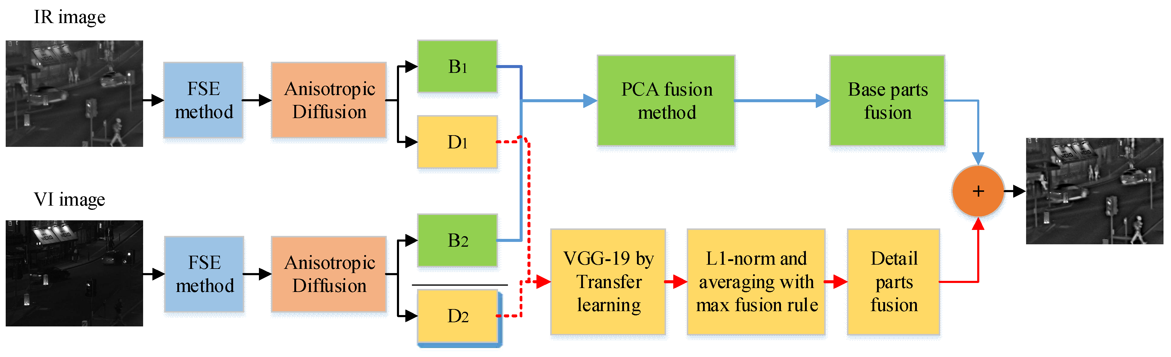
The proposed method first uses a preprocessing contrast enhancement technique named adaptive fuzzy set-based enhancement (FSE). This method automatically enhances the contrast of IR and VI images for better visualization with adaptive parameter calculation. These enhanced images are decomposed into base and detail parts by the anisotropic diffusion method using the partial differential equation. This method prevents diffusion across the edges; it removes the noise and preserves the edges. The PCA method is employed for a fusion of base parts. It can preserve the local energy information while eliminating the redundant data with its robust operation. The four convolution layers of the VGG-19 network through the guidance of transfer learning are applied to detailed parts. This model extracts all the useful salient features with better visual perception, while it saves time and resources during the training without requiring a lot of data. Furthermore, the L 1 n o r m averaging fusion strategy and choose-max selection rule removes the noise in smooth regions while restoring the edges precisely.
The proposed method consists of a series of sequential steps presented in Figure 1. Each step in the proposed method performs a specific task to improve the fused image quality. We will elaborate on each step in detail in sub-sections.

2.1. Fuzzy Set-Based Enhancement (FSE) Method

Capturing the IR and VI image is quite a simple task; however, it is challenging for the human visual system (HVS) to obtain all information due to environments with dense fog, haze, cloud, poor illumination, and noise. In addition, IR and the visible images taken at night vision have low contrast, and they have more ambiguity and uncertainty in the pixel values that arise during the sampling and quantization process. The pixel intensity evaluation needs to be carried out if the image has low contrast. The fuzzy domain is the best approach to alleviate the above-mentioned shortcomings. We have used the FSE method that improves the visualization of IR and VI automatically. This method is adaptive and robust for the parameter calculation of image enhancement.
The fuzzy set for an image I of a × b size with L gray levels each having membership value is given as:
I = i = 1 a j = 1 b μ i j x i j
where, μ i j represents the membership function for each value of intensity at i , j , and x i j 
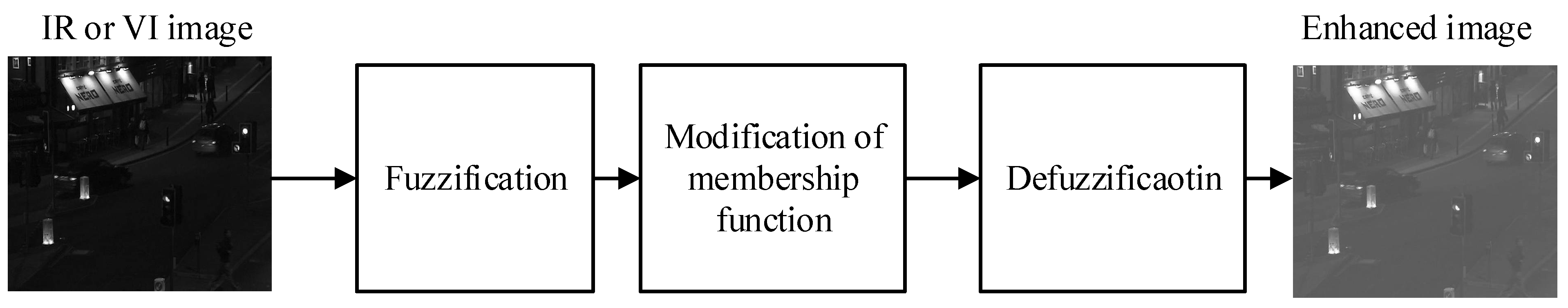
is the intensity value of each pixel. The membership function typifies the appropriate property of images such as edges, brightness, darkness, and textural that can be described globally for the whole image. The block diagram for FSE is given in Figure 2.
We will discuss each step that is involved in FSE in detail as follows:

2.1.1. Fuzzification

The IR or VI images are fed as input I. Then, the image is transformed from spatial domain to fuzzy domain by Equation (2).
μ i j = [ 1 + x max x i j F d ] F e
where, x max indicates the maximum intensity level in an image I, whereas F d and F e represent the fuzzifier dominator and exponential.
The importance of fuzzifiers given in Equation (2) is to reduce the ambiguity and uncertainty in a given image. Many of the researchers have chosen the value of exponential fuzzifier as 2. Instead of selecting a static value for F e , we have determined the adaptive calculation. As we used IR and the VI images (VI taken at night) that have a poor resolution, the general trials using the static value of F e cannot acquire good results. Therefore, keeping the above considerations, we compute the value of F e using the sigmoid [41] function that is calculated by Equation (3):
F e = 1 ( 1 + exp ( m ) )
where, m indicates the mean value of an image.
The dominator fuzzifier F d is obtained as:
F d = x max x min 0.5 1 F e 1

2.1.2. Modification of Membership Function

The contrast intensification operator (CIO) is applied to μ i j to modify the membership function value that is computed by Equation (5):
μ ij = { 2 [ μ i j ] 2 0 μ i j x c 1 2 [ 1 μ i j ] 2 x c μ i j 1 }
The x c is the cross-over point that ascertains the value of μ ij x c . There is a monotonical increment in the μ i j value because of the incremental x c value from 0 to 1 due to CIO, and we have set 0.5 as the value for x c .

2.1.3. Defuzzification

It is a phenomenon of transforming modified fuzzification data from fuzzy domain to spatial domain using Equation (6):
D i j = x max F d × ( ( μ ij ) 1 F e ) + F d
where μ ij indicates the modified member function.

2.2. Anisotropic Diffusion

The anisotropic diffusion (AD) is a way to decompose the source image into a base layer and detailed layer used for image fusion in this paper. This method employs the intra region smoothing procedure to obtain coarse resolution images; hence, the edges are sharper at each coarse resolution. This scheme will acquire the sharp edges while smoothing the homogenous areas more precisely by employing partial differential equations (PDE). An AD employs flux function to ascend the image diffusion that can be computed by Equation (7):
I t = R ( x , y , t ) Δ I + R . I
where I t represents the image diffusion, R ( x , y , t ) = rate of diffusion, = gradient operator, Δ = Laplacian operator, and t is iteration.
We will use forward time central space (FTCS) to solve the PDE. The reason to use FTCS is to maintain diffusion stability, which can be assured by the maximum principle [42]. The equation to resolve the PDE can be computed by Equation (8) as:
I i , j t + 1 = I i , j t + λ [ R N . ¯ N I i , j t + R S . ¯ S I i , j t + R W . ¯ W I i , j t + R E . ¯ E I i , j t ]
where λ represents the stability constant in the range 0 λ 0.25 , D i , j t + 1 indicates the image coarse resolution in forward time at t + 1 iteration that relies on former I i , j t . The ¯ N , ¯ S , ¯ E , and ¯ W show the neighboring differences in the north, south, east, and west directions, and it can be computed by Equation (9):
{ ¯ N I i , j = I i 1 , j I i , j , ¯ S I i , j = I i + 1 , j I i , j , ¯ E I i , j = I i , j + 1 I i , j , ¯ W I i , j = I i , j 1 I i , j }
Similarly, the flux functions R N , R S , R E , and R W will be updated at each iteration in all four directions as:
{ R N i , j t = h ( ( I ) i + 1 / 2 , j t ) = h ( | ¯ N I i , j t | ) , R S i , j t = h ( ( I ) i 1 / 2 , j t ) = h ( | ¯ S I i , j t | ) , R E i , j t = h ( ( I ) i , j + 1 / 2 t ) = h ( | ¯ E I i , j t | ) , R W i , j t = h ( ( I ) i , j 1 / 2 t ) = h ( | ¯ W I i , j t | ) , }
The h ( . ) in Equation (10) is the monotonical decrement function with h ( 0 ) = 1 , and can be computed as:
h ( I ) = 1 1 + ( I p ) 2
h ( I ) = e ( I p ) 2
where p represents a free parameter used to determine the validity of the region boundary based on its edge intensity level.
Equation (11) is more useful if a given image contains wide regions instead of narrow regions. Wherein, Equation (12) is more flexible if an image has high-edge resolution than poor-edge resolution; however, the parameter p is fixed.
Let the input images I n ( x , y ) n = 1 having p × q size be fed into AD that are well-aligned and co-registered. These images are infiltrated into the edge-preserving smoothing AD process for acquiring the base layer, and it is computed as Equation (13):
B n ( x , y ) = A d f ( I n ( x , y ) )
where A d f ( I n ( x , y ) ) indicates the AD process for the n-th base layer, while B n ( x , y ) is the acquired n-th base layer. After acquiring the base layer, the detail layer is computed by subtracting the base layer from the source image as given in Equation (14):
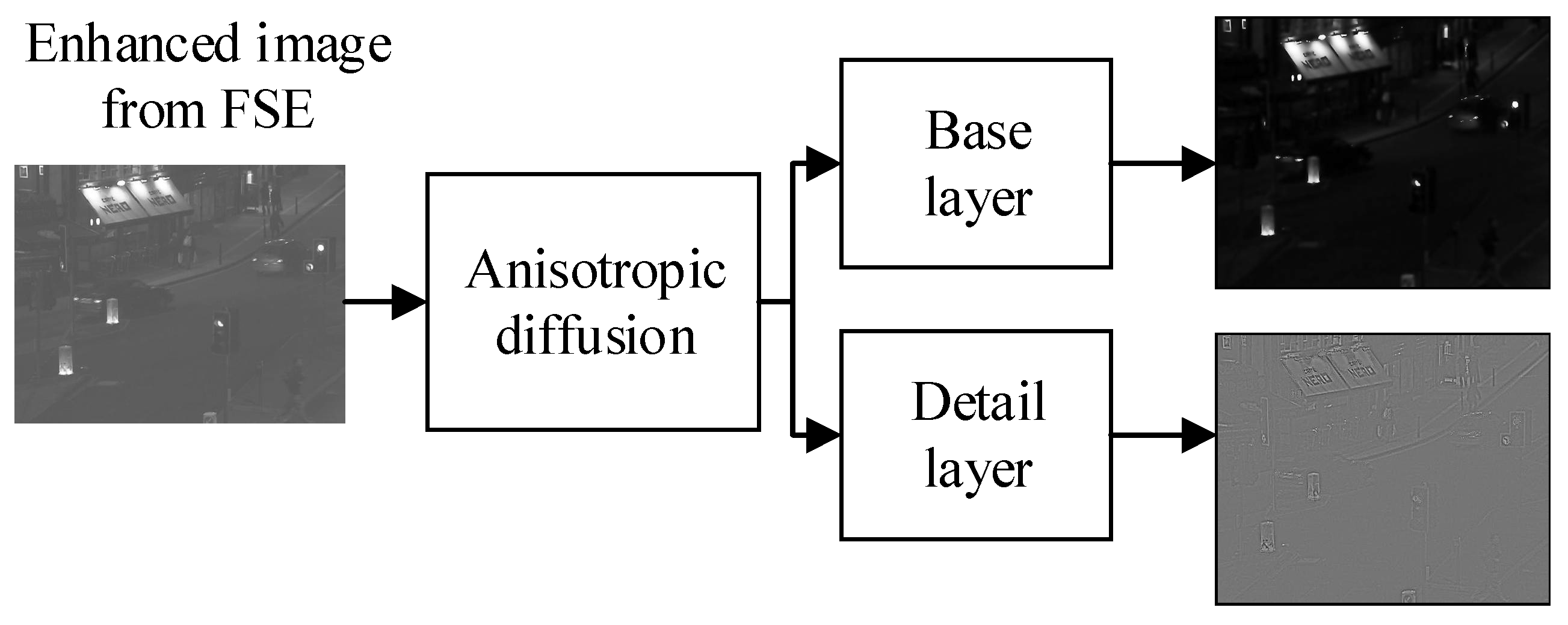
D n ( x , y ) = I n ( x , y ) B n ( x , y )
It can be seen in Figure 3 that AD is employed in an enhanced image obtained from the FSE scheme. The AD decomposes the image into the base layer and detail layer, and their base and detail images are shown in Figure 3. We have applied AD to only one enhanced image of FSE, and we will apply the AD to another image in the same pattern to obtain a base and detail layer for another image.

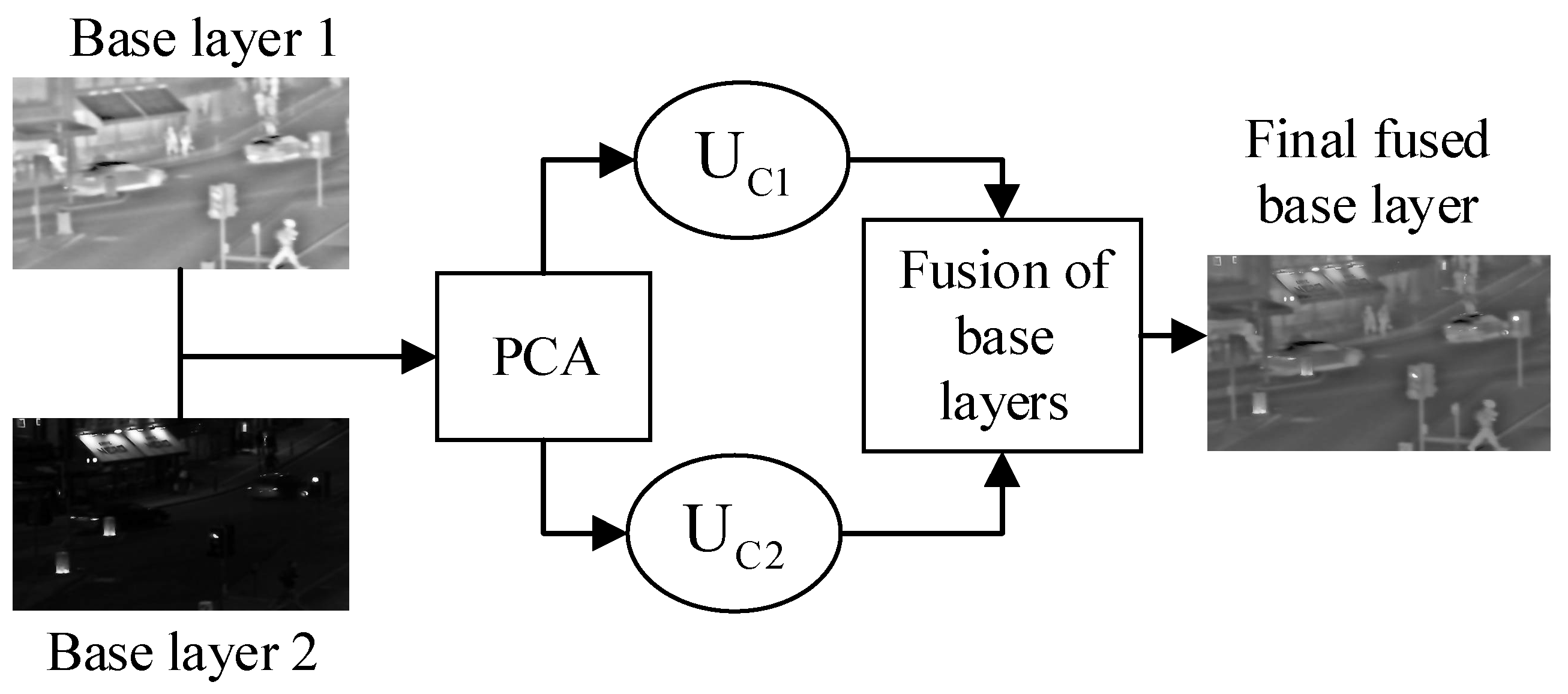
2.3. Fusion Strategy of Base Layers

The base layers contain the energy information, and it is vital to preserve the energy information from both base layers to extract more features. Though the average fusion scheme can be applied, it cannot preserve the complete information. The PCA is utilized for the fusion of low-frequency images that is a dimension reduction technique that minimizes the complexity of a model and avoids overfitting. This method compresses a dataset into a lower-dimensional feature subspace while preserving relevant information at a high level of detail. It takes a subset of the original features and uses that knowledge to create a new feature subspace. It locates the most elevated variance directions in high-dimensional data and projects them onto a new subspace with the same or fewer dimensions as the original. The PCA transforms correlated variables into uncorrelated forms that choose features with significant values of eigenvalues λ and eigenvectors ξ . After that, the principal components U C 1 and U C 2 are computed from these highest eigenvalues λ and eigenvectors ξ . All the principal components are orthogonal to each other, which helps to eliminate redundant information and makes fast computation. The PCA method used for the fusion of base layers is discussed below.
1. The proposed method is applicable for a fusion of two, or more than two, base layers; however, we consider only two base layers for simplicity. Let B 1 ( x , y ) and B 2 ( x , y ) be the two base layers obtained after decomposition from the AD process. The first step is to acquire a column matrix, Z, from these two base layers.
2. Obtain the variance V and covariance C v matrix C Z from column matrix Z for both base layers B 1 ( x , y ) and B 2 ( x , y ) . The V and C v is calculated by Equation (15):
Z = [ V 1 C v ( 1 , 2 ) C v ( 1 , 2 ) V 2 ]
C v = ( ( x 1 x ¯ 1 ) × ( x 2 x ¯ 2 ) ) T 1
In Equations (15) and (16), V 1 , V 2 , C V ( 1 , 2 ) indicates the variance and covariance, whereas T represents the number of iterations.
3. After obtaining the variance and co-variance, the next step is to obtain the eigen values λ and eigen vectors ξ . The λ is computed by Equation (17):
D e t | Z λ I | = 0
( ( V 1 λ ) × ( V 2 λ ) ) × C v ( 1 , 2 ) 2 = 0
Now we compute the ξ by Equation (19):
ξ 1 = [ ξ 1 ( 1 ) ξ 2 ( 2 ) ]   and   ξ 2 = [ ξ 2 ( 1 ) ξ 2 ( 2 ) ] for   C Z
4. The next step is to determine if the uncorrelated components U c 1 and U c 2 match the highest eigenvalues ( λ max = max ( λ 1 , λ 2 ) ) . Let ξ max represent the eigenvector corresponding to λ max , then U c 1 and U c 2 are computed as:
U c 1 = ξ max ( 1 ) n ξ max ( n ) , U c 2 = ξ max ( 2 ) n ξ max ( n )
5. The final fused base layer can be calculated by Equation (21) as:
B ¯ ( x , y ) = U c 1 B 1 ( x , y ) + U c 2 B 2 ( x , y )
The block diagram for a fusion of base layers by PCA method is shown in Figure 4. The two base layers that are decomposed by AD are fed to PCA and the final fused base layer is obtained after the fusion process of PCA. The symbols U c 1 and U c 2 in Figure 4 represent the uncorrelated components for both base layers. These uncorrelated components are obtained from the highest eigenvalues and eigenvectors that are orthogonal to each other, and its computation would be fast due to the elimination of redundant data.

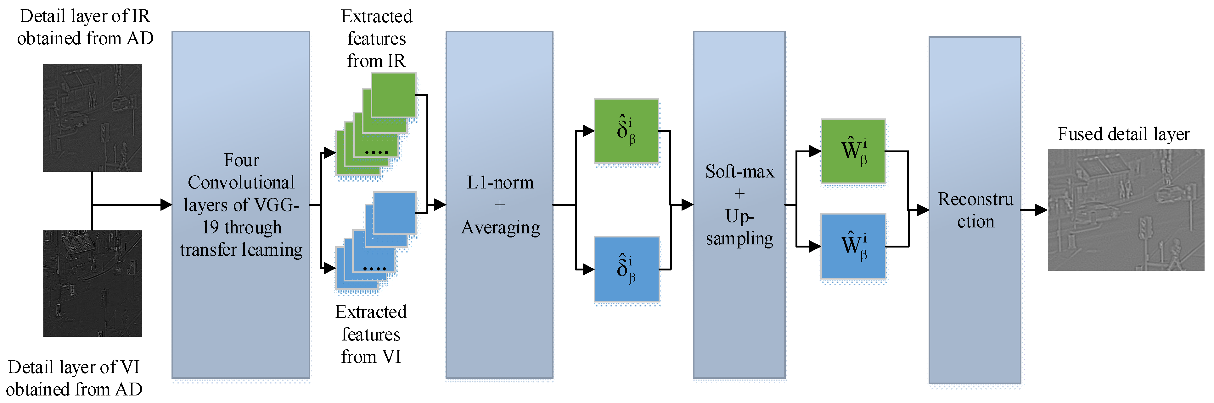
2.4. Fusion Strategy for Detail Layers

Most traditional methods use the choose-maximum fusion rule to extract the deep features. Nonetheless, this fusion scheme significantly loses detailed information that affects the overall fused image quality. In this paper, we extract the deep features by four convolutional layers of VGG-19 through the guidance of transfer learning. The activity level maps are acquired from desired extracted deep features by L 1 n o r m and the averaging method. Then, soft-max and up-sampling are employed to these activity level maps to generate the weight maps. After that, these weight maps are convolved with IR and VI images to obtain the four candidates. Finally, the maximum strategy is applied to these four candidates to obtain the final fused detailed layer. The whole phenomena for a fusion of detailed layers are shown in Figure 5.
We will discuss each step more precisely in sub-sections.

2.4.1. Feature Extraction by VGG-19 through Transfer Learning

We have used a VGG-19 network that consists of convolution layers, ReLU (rectified linear unit) layers, pooling layers, and fully connected layers [43]. The main purpose for using the VGG-19 network is its feasibility which has a 3 × 3 receptive field for each convolution layer with a fixed stride of 1 pixel and spatial padding of 1 pixel. We took only four convolution layers from VGG-19 through the guidance of transfer learning. Transfer learning helps to reduce the training effort. We took four convolution layers (conv1-1, conv2-1, conv3-1, and conv4-1) and chose the first convolution layer from each convolution group because the first convolution layer contains complete significant information.
Let β represent the number of detailed images, and we took two detailed images that are X 1 d and X 2 d . Assume that φ β i , m represents the feature map of the β t h detailed layer at i t h convolution layer, and m shows the number of channels of the i t h layer, so m { 1 , 2 , ..... , M } . The M is the maximum number of channels, and it can be calculated as 64 × 2 i 1 by Equation (22).
φ β i , m = Φ i ( X β d )
Each Φ i ( . ) represents a layer in VGG-19, and we chose four layers, i.e., i { 1 , 2 , 3 , 4 } conv1-1, conv2-1, conv3-1, and conv4-1.
Suppose φ β i , 1 : M ( x , y ) indicate the contents of φ β i , m at ( x , y ) position, and φ β i , 1 : M ( x , y ) is an M-dimensional vector. Consequently, the phenomena of our fusion strategy is elaborated in the next section, which is also shown in Figure 5.

2.4.2. Feature Processing by Multiple Fusion Strategies

Inspired by [44], we employ the L 1 n o r m method to quantify the amount of information in the detailed images, which is called the activity level measurement of detailed images. After acquiring the feature maps φ β i , m , the next step is to find the initial and final activity level maps. The initial activity level map δ β i is obtained by using the L 1 n o r m scheme that is computed as given in Equation (23) and depicted in Figure 5:
δ β i = φ β i , 1 : M ( x , y ) 1
The next step is to find the final activity level map δ ^ β i . The δ ^ β i is computed by Equation (24):
δ ^ β i = u = r r v = r r δ β i ( x + u , y + v ) ( 2 r + 1 ) 2
where r represents the size of the block, which helps our fusion method avoid misregistration. The larger value of r makes fusion more robust to prevent misregistration. Though some detail could be lost by choosing a higher value of r, we need to determine the value of r carefully. In our case, we have selected r = 1 because it preserves all information at this value while it also avoids misregistration.
It can be seen in Figure 5 that we have applied a soft-max that is used for computing the weight map W β i from δ ^ β i . The W β i is calculated by Equation (25):
W β i ( x , y ) = δ ^ β i ( x , y ) n = 1 γ δ ^ β i ( x , y )
where γ indicates the number of activity level maps. As we have taken two source images, therefore, γ = 2 in our case, we will obtain four pairs of initial weight maps to distinguish scales because we have chosen four convolutional layers through transfer learning.
The pooling layer is used in the VGG-19 network that acts as a sub-sampling; hence, it reduces the size of feature maps. Therefore, after every pooling layer, the feature maps are resized to 1 s times where s denotes the pooling stride, and the stride of the pooling operator is 2. Thus, the size of the feature maps would be 1 2 i 1 for each different layer of the convolution group, so i { 1 , 2 , 3 , 4 } for the first, second, third, and fourth convolution layer in each convolution group. Therefore, after obtaining the initial weight maps, we use the up-sampling operator to resize the weight map size that equals the size of detail content. The final weight maps using the up-sampling operator can be computed by Equation (26):
W ^ β i ( x + p , y + q ) = W β i ( x , y ) , p , q { 0 , 1 , ( 2 i 1 1 ) }
Now, the four weight maps that are acquired by the up-sampling operator are convolved with the detail layer of IR and VI images to obtain the candidates, and it is computed by Equation (27):
D i ( x , y ) = n = 1 γ W ^ n i ( x , y ) × X n d ( x , y ) , γ = 2
The fused detail content D ¯ is finally computed by employing a choose-max value from four candidate fused images, as shown in Figure 5 and Equation (28).
D ¯ ( x , y ) = max | D i ( x , y ) | , i { 1 , 2 , 3 , 4 }

2.5. Reconstruction

The reconstruction of the final fused image is obtained by simple linear superposition of the fused base image and the fused detailed image as given in Equation (29).
F ( x , y ) = B ¯ ( x , y ) + D ¯ ( x , y )

3. Results

The experiments are conducted on IR and VI datasets that prove the efficacy of the proposed method over conventional and recent image fusion methods. Though there is no universal evaluation standard for comparing the image fusion quality, subjective and objective evaluation is the best approach to compare the results of image fusion methods accurately. We took all the IR and VI from the TNO dataset [45], and all the images are preregistered that can be directly used for fusion. We compared our proposed method with the cross bilateral fusion (CBF) [15] scheme, discrete cosine transform (DCT)-based [18] method, improved DWT [19] fusion method, convolution sparse representation (CSR) [27], and latent low-rank representation (LatLRR)-based [28] methods. The simulation results are implemented using MATLAB 2016b on a core i5 3.2 GHz processor with 8 GB RAM.

3.1. Subjective Evaluation

The subjective evaluation is a good approach to compare the difference among different image fusion methods by the human visual system (HVS). The quality of images can be judged based on image brightness, contrast, and other features that can reflect the visual effect of the image.
It can be seen in Figure 6c that the fused image acquired by CBF has more artifacts and the image details are not clear. This is because the CBF method obtains weight by directly measuring the strength of horizontal and vertical details, leading to artifacts and noise. The fused image obtained by the DCT method in Figure 6d is also affected by gradient reversal artifacts, and it contains halo effects. Since the DCT method uses cross-correlation using a low filter that can capture the energy information from source images, the detailed information cannot be preserved, such as edges and contours that affect the overall quality of a fused image. The fused image produced by improved DWT in Figure 6e has better visual effects than CBF and DCT, but the image is blurred, and the details are unclear. It is well known that the DWT method has limited ability to preserve detailed information because it has limited directional information. Moreover, it cannot preserve more spatial (energy information) details because this method fails to capture energy information; due to that, the image is blurred. The fused result obtained by the CSR-based method in Figure 6f produces good results, and it is less noisy, but the overall information in the image is still blurred, and characters on billboards are not vivid, as can be seen in the red box. Since the CSR method used an averaging strategy to avoid insensitivity to misregistration, it uses a window with size r. The window size r results in losing some spatial details because the energy and edges of objects have different sharpness. The LatLRR-based method in Figure 6g achieves good results, and the letters on the billboard are also more vivid than existing methods, but the contrast of an image is still not satisfactory. It is due to using the weighted averaging strategy for a fusion of low-rank, and it is well known that the weighted-averaging approach is limited to preserve more spatial information. The fused image acquired by the proposed method has high quality in terms of detail extraction such as edges and contours due to the novel fusion strategy of L 1 n o r m and the averaging strategy along with the choose-max selection fusion rule in the VGG-19 network. Besides, the proposed method has very negligible noise due to the unique characteristics of the fuzzy set approach. It uses the exponential fuzzifier that utilizes adaptive calculation to remove the noise and adjust contrast.
The CFB method in Figure 7c contains more artificial noise points, and the significant features are not obvious. Its visual effect is poor compared with other fusion methods. The fused image obtained by the DCT method has the presence of gradient reversal artifacts. In addition, the details are fuzzy, and there are numerous artificial edges and contours in the whole image. The fused images obtained by the CSR and LatLRR methods almost look similar. They have fewer artifacts and noise, resulting in a more informative image. They restore the thermal objects with more details, but they lose some spatial details such as small windows, and other details are not very clear, as can be seen in the red boxes. The fused image obtained by the DWT method captures more salient features from both source images. On the other side, there is a large amount of additional structure around the prominent targets, which is not present in the source images but is introduced by noise, resulting in a distorted image. It can be seen in Figure 7h that the proposed method preserves whole energy information due to the unique characteristics of PCA because it transforms the correlated variable into an uncorrelated form that chooses those features which have significant values of eigenvalues λ and eigenvectors ξ . In addition, the fused image restores more contrast, structural information, smooth patterns, and contours.
It can be depicted in Figure 8 that the CBF method has obvious artifacts and salient features are unclear. The fused image obtained by DCT also has noise and gradient reversal artifacts. Hence, the targets are ambiguous to detect from fused images, thus resulting in a worse visual effect. The fused image acquired by the CSR method has a better visual effect than CBF and DCT. Contrarily, the details are still fuzzy in the fused image, and the contrast is low. Moreover, it can be seen in the red box in Figure 8f that the bench is blurred. The CSR method uses the choose-max strategy for the fusion of low frequency, and this fusion rule is not effective in capturing energy information. The DWT and LatLRR methods have more details, and the bench, which is highlighted by a red box is vivid. The contrast of DWT is more than the latent-rank method, but the DWT image has more artificial noise, especially surrounding the bench, while the latLRR method has less noise than DWT and the other three methods. The proposed method achieves a better result than the aforementioned methods. The red highlighted bench is clear, and the water transparency in the lake is also more vivid because the proposed method uses AD that employs the intra region smoothing procedure to obtain coarse resolution images. We examined various values for free parameters λ , t and k, and we have chosen λ = 0.15 , t = 10 and k = 30 for smoothing because it gives good results at these values. This makes the edges sharper at each coarse resolution. Furthermore, the contrast of the image is bright with very little noise, which shows that the image can preserve all salient features from both source images.
Figure 9c–h shows the fusion results of other methods and proposed methods. The CBF method contains substantial gradient reversal artifacts that result in distortion in the image. The DCT method contains most of the information from the IR image while it loses information from the VI image. Hence, the fused image results in the loss of detailed information, and the overall quality of an image is worse. The DWT and LatLRR methods almost resemble the fused image, thereby obtaining better results than CBF and DCT methods. Nevertheless, the fused image is fuzzy and blurred as can be observed in the red boxes, and it has less contrast that fails to capture all salient features from the source images. The fused image obtained by the CSR method has better fusion results than the other four methods and has better contrast. On the contrary, the IR component of the CSR method has domination, and due to that, it cannot preserve more detailed features from the VI image. The fused image produced by the proposed method has very little noise. Besides, due to using a novel L 1 n o r m and averaging strategy along with the choose-max selection fusion rule in the VGG-19 network, the fused image preserves all salient features such as edges and textures from both source images. Moreover, it can capture all patterns with better contrast, as can be seen in the red boxes. Hence, the proposed methods show their efficacy compared with all other methods.
It can be seen in Figure 10c,d that the fusion quality of CBF and DCT is significantly worse due to the misalignment of the source images. There are gradient reversal artifacts and noise in the CFB image due to high sensitivity because the CBF method obtains weight by measuring the strength of horizontal and vertical details directly that introduces noise and artifacts. In contrast, the DCT image quality is affected as it uses cross-correlation with a low pass filter, so it discards useful energy information that produces blurred images. The DWT, CSR, and LatLRR methods have almost similar fused quality visually, but the DWT has more noise because DWT uses down sampling, due to which there is a shift variance that introduces artifacts. Besides, the textures are not smooth due to the loss of detailed information during down sampling phenomena that cause Gibb’s effect. The proposed method again shows dominance compared with other fusion methods. It can be observed in the red boxes that the proposed method has smooth patterns, textures, and edges due to the unique fusion rule of L 1 n o r m and averaging strategy along with the choose-max selection fusion rule in the VGG-19 network. Furthermore, the left–right bottom red boxes show that the proposed method restores more salient features with very smooth background because of choosing the specific values for free parameters ( λ , t and k) in the anisotropic diffusion process. In addition, the contrast of a fused image is more vivid due to the fuzzy set enhancement method that uses an adaptive calculation for the exponential fuzzifier that proves the efficacy of the proposed method compared with other methods.
Due to space limitations, we cannot discuss the results of each fused image. We have only presented the final fused image of the proposed method and five other methods in Figure 11. It can be observed that the proposed method achieves better results than other methods.

3.1.1. Statistical Evaluation

We use two statistical tests, such as the Wilcoxon signed-rank test [46] and the Friedman test [47], to illustrate the superiority of the proposed method over other state-of-the-art (SOTA) methods. The Wilcoxon signed-rank test observes the significant difference between the input images and the generated images. In contrast, the Friedman test computes a significant variation in image quality between different approaches. For the former, we created two kinds of image pairs for a test, the IR image vs. the fused image, and the VI image vs. the fused image, to see the effects of different methods on image fusion. The lower the p-value, the more likely it is to reject the null hypothesis, implying that the output images differ from the input images and carry more information about the IR/VI images. It can be seen in Table 2 that the p-value of the IR-fused images produced by the proposed method is the lowest, indicating that our approach can effectively fuse the input images from different sources (IR and VI). For the latter, we employ peak-signal-to-noise-ratio (PSNR) as the ranking metric to test the significant difference among the other methods. As shown in Table 2, the result is small enough to exhibit the superiority of the proposed method over SOTA methods.

3.1.2. User Case

We performed a user case in which we invited ten field experts to provide a ranking for each method on five pairs of images. The detailed discussion is described below:
We conducted a user study on five datasets to demonstrate that our method outperforms other methods. We invited ten experts to rank the results of all approaches according to their choice. Each expert was asked to rate six results (the proposed approach and five other methods) using a scale of one point (least preferred) to six points (most favorite) for each pair of source images. Experts conducted the subjective analysis on the following four points: (1) precise details, (2) no loss of information, (3) contrast of an image, and (4) noise in the fused image. The experts were assigned anonymous results in random order to avoid subjective bias.
Furthermore, the user study was performed in the same environment (room, light, and monitor). We calculated the average points obtained by each approach on five pairs of source images after the experts finished grading all of the simulation results. Table 3 presents the average points obtained by each method by experts on five pairs of source images.
It can be observed from Figure 12 that experts prefer the average results produced by the proposed method.

3.2. Objective Evaluation

The objective evaluation is used to analyze the difference based on mathematical calculation quantitatively. We compared our method with conventional fusion methods on six objective evaluation assessment parameters.

3.2.1. Feature Mutual Information (FMI)

The FMI [48] is used to measure the mutual information of the image features such as edges, contrast, details, and so on. It can be computed by Equation (30):
F M I = M I A , F + M I B , F
M I X F = x , f H X , F ( x , f ) log H X , F ( x , f ) H X ( x ) H F ( f ) , X { A , B }
where, H X ( x ) and H F ( f ) represent the marginal histogram of an input image X and the fused image F . The H X , F ( x , f ) denotes the joint histogram of X and F . X indicates the feature map of input image A and B , whereas, A , B , F are the feature maps of IR, VI, and the fused image, respectively.

3.2.2. Modified Structural Similarity Index ( S S I M a )

The S S I M a [49] is used to compute the distortion and loss in the image structure. The quality of the fused image would be better if the value of S S I M a is larger because larger values correspond to a fused image with more structure. The fused image will have more distortion and loss if the value of S S I M a is smaller. The higher value of S S I M a is written in bold letters in Table 4. It can be calculated as Equation (32):
S S I M a ( F ) = ( S S I M A , F + S S I M B , F ) × 0.5
where S S I M ( . ) denotes the structural similarity, F represents the fused image, and A , B denotes the IR and VI image.

3.2.3. Average Pixel Intensity (API)

The A P I [3] is used to measure the contrast of the fused image. The quality of the fused image would be better if the value of API is larger. It is obtained by Equation (33):
A P I = i = 1 m j = 1 n f ( i , j ) m × n
where f ( i , j ) is the intensity of the pixel at ( i , j ) , and m × n represents the image size.

3.2.4. Entropy (EN)

The entropy [18] determines the amount of information available in the image. It is computed by Equation (34):
E N = l = 0 L 1 p l log 2 p l
where, L represents the number of gray levels and p l indicates the normalized histogram of the corresponding gray level in the fused image. The larger value of EN refers to a fused image with more information.

3.2.5. Quality Ratio of Edges from Sources Images to Fused Image ( Q F A B )

The Q F A B [37] is used to compute the amount of edges information transferred from input images to the final fused image. It is calculated by Equation (35):
Q F A B = i = 1 N j = 1 M Q A F ( i , j ) w A ( i , j ) + Q B F ( i , j ) w B ( i , j ) i = 1 N j = 1 M ( w A ( i , j ) + w B ( i , j ) )
where Q A F , Q B F represents the amount of edge information transferred from image A to F, and B to F at location ( i , j ) , respectively. The A, B, and F are input into image 1, image 2, and the fused image, respectively. The w A and w B indicate the weights in image A and image B. The higher the value of Q F A B , the more edges information will be transferred from the input images to the fused image.

3.2.6. Noise ratio from the source image to the fused image N A B F

The N A B F [18] is the index of fusion on the basis of artifacts and noise. The larger value corresponds to more artifacts and noise in the fused image, while the image will have less artifacts and noise if the value is smaller. The smaller value is written by bold letters in Table 4 for ease of reading. It is computed by Equation (36):
N A B F = n , m N n , m ( w n , m A + w n , m B ) n , m ( w n , m A + w n , m B )
where N n , m indicates the fusion loss and w n , m A and w n , m B represent the weight maps of the IR and VI images.
Table 4. The average values of FMI, S S I M a , API, N F A B , EN, and Q F A B .
MethodsCBF [15]DCT [18]Improved DWT [19]CSR [27]LatLRR [28]Proposed
FMI0.26510.27460.30410.34390.35610.3951
S S I M a 0.58270.59710.63490.74120.77980.8469
API56.371056.492858.931463.017866.715371.9081
N F A B 0.30490.30150.29160.01970.00380.0021
EN4.01174.15374.84716.15176.89247.9907
Q F A B 0.65380.71420.78670.81910.83060.8727
We performed fusion on 18 test images, and their average values of FMI, S S I M a , API, EN, Q F A B , and N F A B are presented in Table 5. Due to space limitations, we provided the average values for all mentioned parameters. In addition, we also provided a line graph and scattering plot in Figure 13, Figure 14, Figure 15, Figure 16, Figure 17 and Figure 18, respectively. The primary purpose of using the two different graphs is for ease of comprehension.
The larger values of F M I , S S I M a   A P I , EN, and Q F A B result in a good quality fused image with more salient features from both source images, while the smaller values correspond to a fused image with less similar structure. On the contrary, the fused image will have less artifacts and noise if the value of N F A B is smaller, while the higher value results in a fused image with more artifacts and noise. The larger values for F M I , S S I M a , A P I , EN, Q F A B , and the smaller values of N F A B are written in bold letters in Table 4 for differentiation purposes. It can be observed in Table 4 and Figure 13 that CBF and DCT have fewer values for F M I , which means the fused image restores less salient features from source images. The improved DWT produces better results than CBF and DCT; however, the CSR and latent-based methods achieve better results than DWT. The proposed method outperforms all other methods that acquire a better quality fused image with more salient features. Similarly, it can be observed in Table 4, Figure 14 and Figure 15, that the proposed method achieves significant values for S S I M a and A P I which shows the optimal fusion performance compared with other methods by retaining more structure and contrast from the source images. Compared with other methods, the latent-based method’s performance is better than the other three methods, whereas the CSR values are closer to the latent-based method.
Similarly, it can be seen in Table 4, Figure 17 and Figure 18, that the proposed method has higher values for EN and Q F A B than the other methods. The yellow triangles indicate the proposed method in scattering plotting in Figure 17 and Figure 18. It can be seen that the proposed method achieves higher values for EN Q F A B except for a few images. Moreover, the CBF (square boxes) and DCT methods (circle boxes) in Figure 17 and Figure 18 produce poorer results than all other methods. Furthermore, it can be observed from Table 4 and Figure 16 that the proposed method has significantly fewer values of N F A B , which proves that the fused images have fewer artifacts and noise than other methods. In this regard, it can be concluded that the proposed method produces better visual results and obtains better values for objective evaluation analysis, demonstrating the supremacy of the proposed method.
We also present the evaluation criteria for FMI, S S I M a , API, EN, Q F A B , and N F A B for objective quality parameters to estimate the results. The evaluation criteria for quality parameters in presented in Table 5.
It can be observed from evaluation criteria that the proposed method obtained the best performance for all evaluation parameters while the performance of CBF and DCT methods exhibited poor performance.

3.3. Computation Time Comparison

The average computation time for the proposed method and the other compared fusion methods is presented in Table 6. The experiments are conducted for computation time (t) in seconds on MATLAB 2016b with corei5 3.20 GHz processor and 8 GB RAM. It can be depicted in Table 6 that the computation time for LatLRR is longer than other methods, which shows it has the poorest timeliness. The CBF method is the fastest, which shows it has the best timeliness; however, its performance is the worst on subjective and objective parameters. The computation time of the proposed method is longer than CBF, DCT, and improved DWT, but the better visual effects can compensate for the reduced timeliness. The computation time for the proposed method is shorter than CSR and LatLRR, while it also produces better visual and objective performance. Therefore, the computation time for the proposed method is still acceptable.

4. Discussion

Implementing the image fusion method that extracts all salient features from individual source images into one composite fused image is the hot research topic of future development in IR and VI applications. This proposed work is one of the attempts in the IR and IV image fusion research area. Our method not only emphasizes the crucial objects by eliminating the noise but also preserves the essential and rich detailed information that is helpful for many applications such as target detection, recognition, tracking, and other computer vision applications.
Various hybrid fusion methods amalgamate the advantages of different schemes to enhance the image fusion quality. In our hybrid method, each stage improves the image quality, which can be observed in Figure 2, Figure 3, Figure 4 and Figure 5, respectively. Our hybrid method extensively uses the fuzzy set-based enhancement, anisotropic diffusion, and VGG-19 network through transfer learning with multiple fusion strategies and PCA. The FSE method automatically enhances the contrast of IR and IV with its adaptive parameter calculation. In addition, this method is robust in environments with fog, dust, haze, rain, and cloud. The AD method using PDE is applied that decomposes the enhanced images of FSE into the base and detailed images. It has the attribute of removing noise from smooth regions while retaining sharp edges. The PCA method is employed in the fusion of the base parts that restrain the distinction between the background and targets since it can restore the energy information. Besides, it eliminates redundant information with its robust operation. The VGG-19 network using transfer learning is adapted as it has a significant ability to extract specific salient features. In addition, we have used four convolution layers of VGG-19 through transfer learning that efficiently saves time and resources during the training without requiring a lot of data. At last, the L 1 n o r m and averaging fusion strategy along with the choose-max selection fusion rule is applied, which efficiently removes the noise and retains the sharp edges.
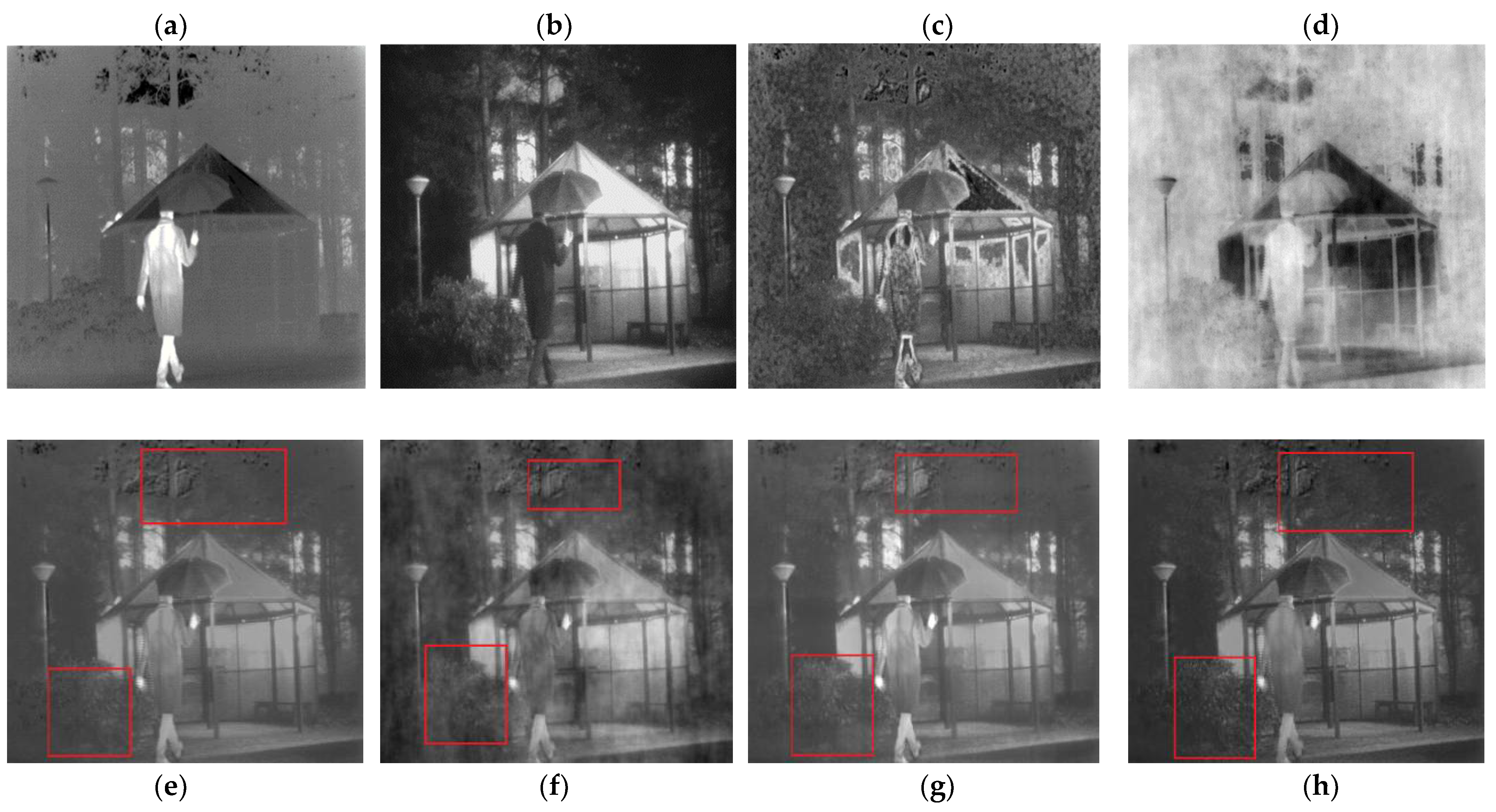
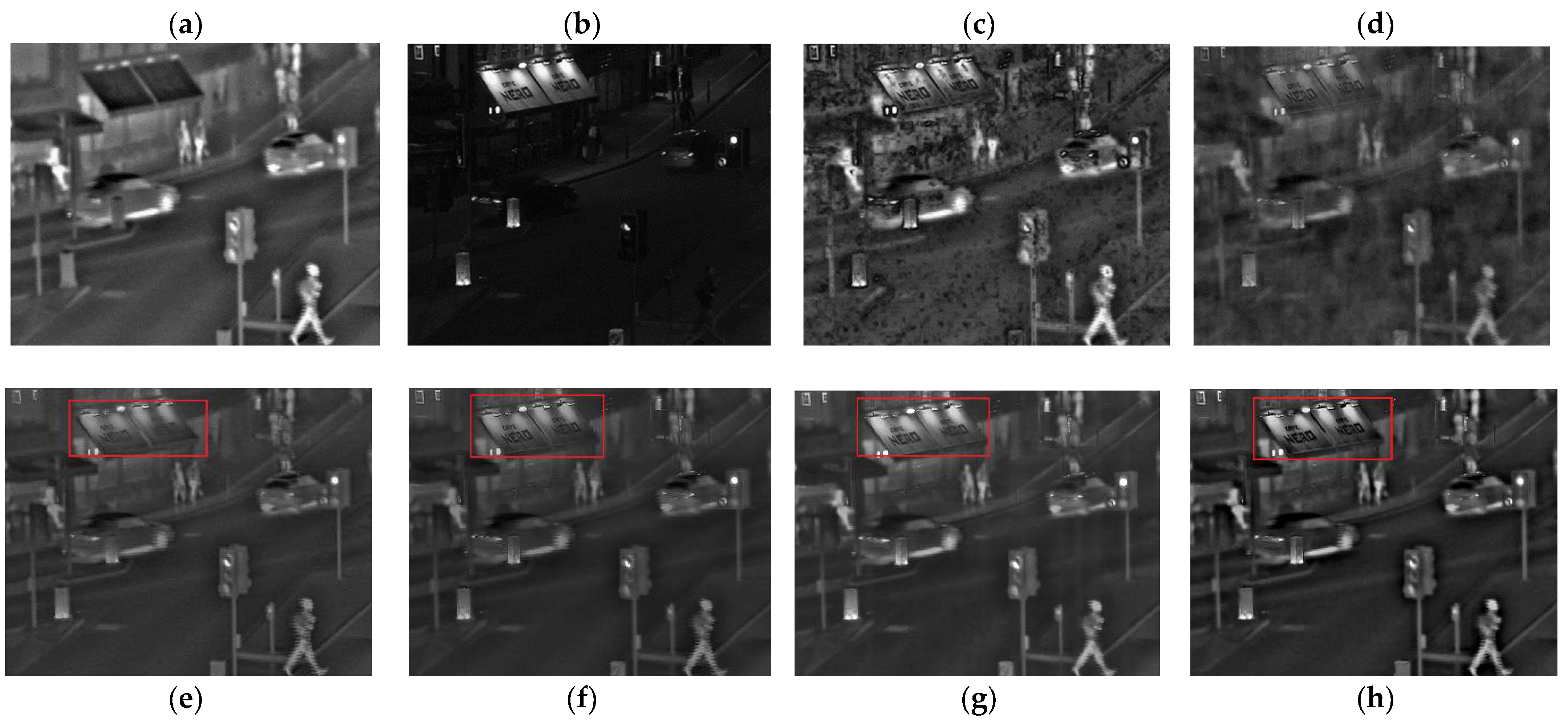
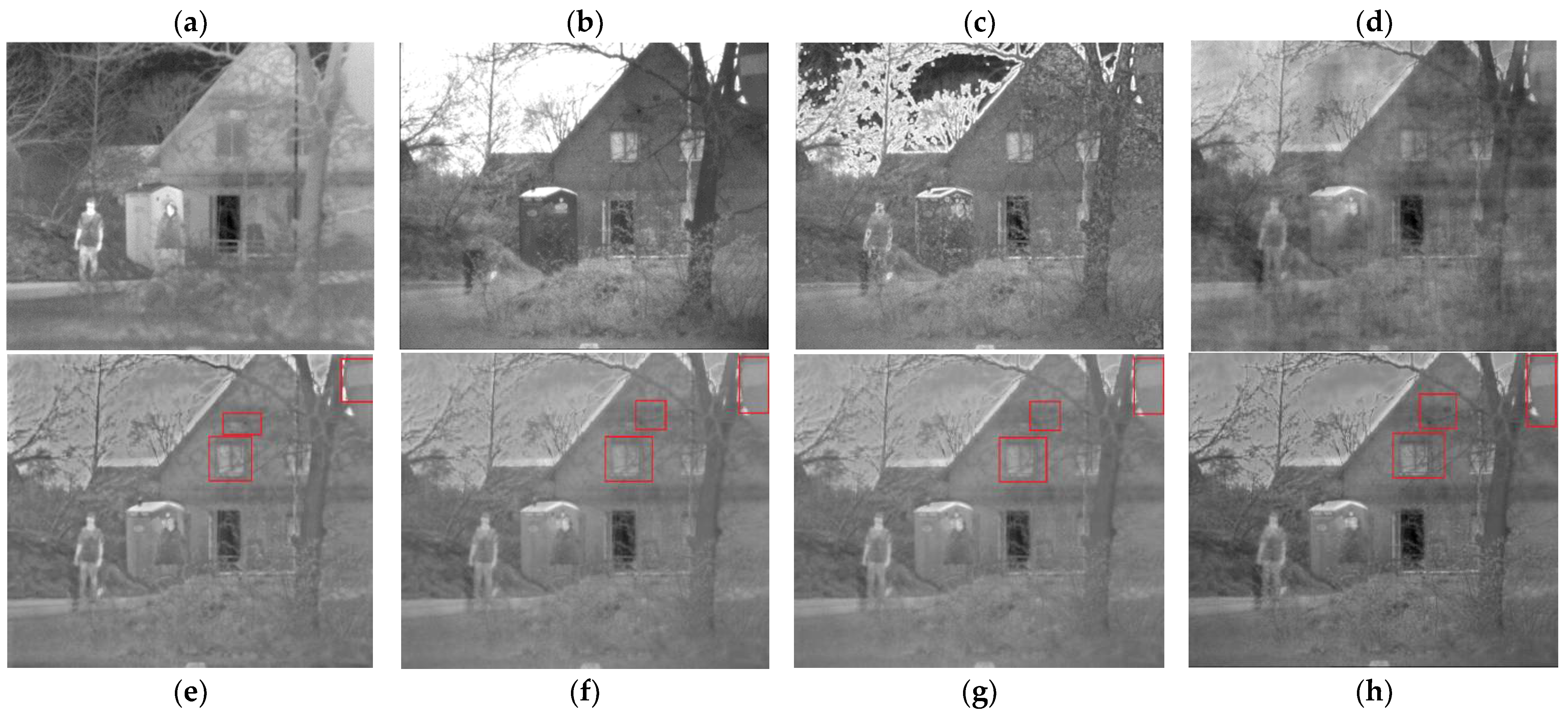
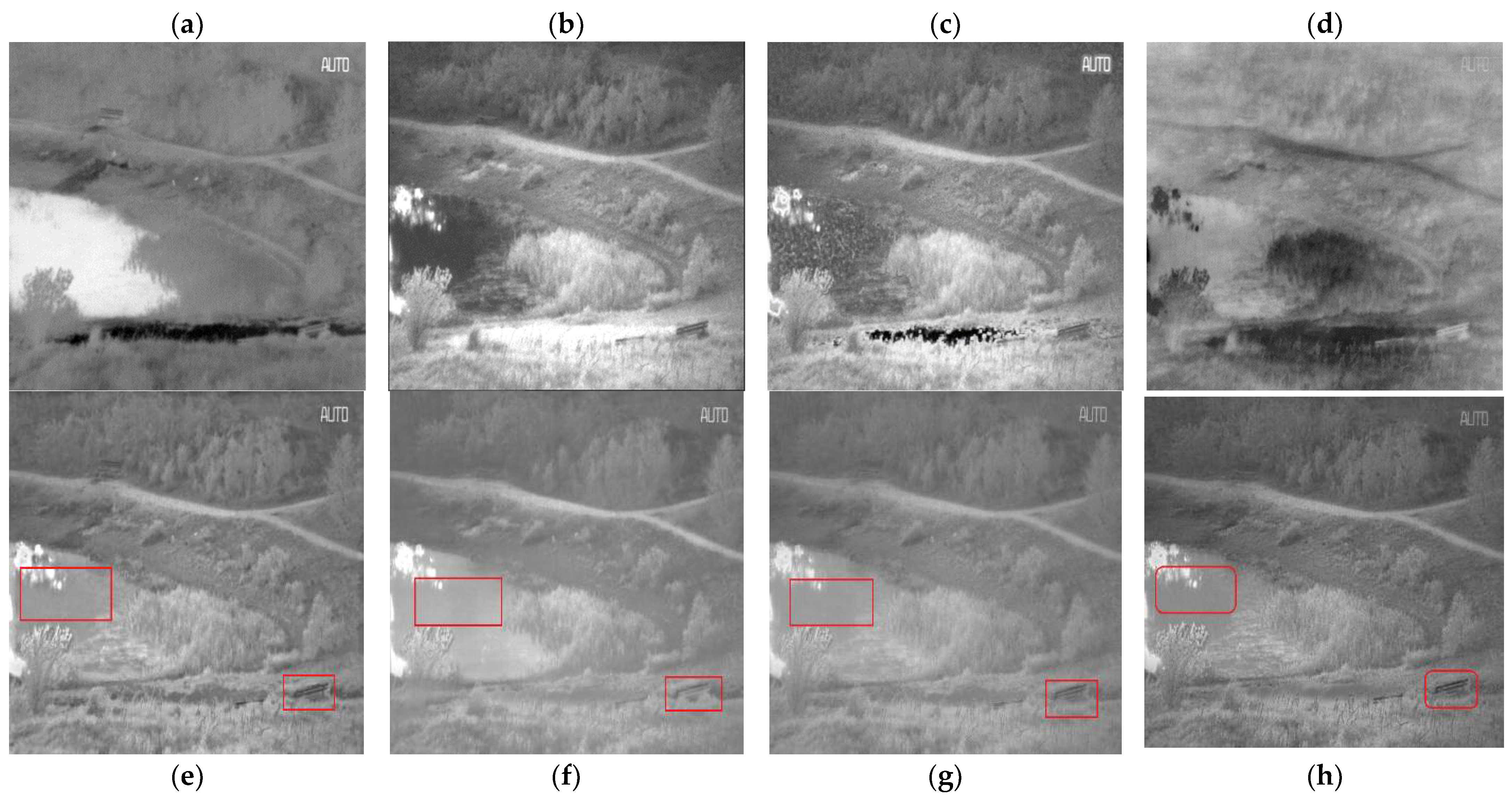
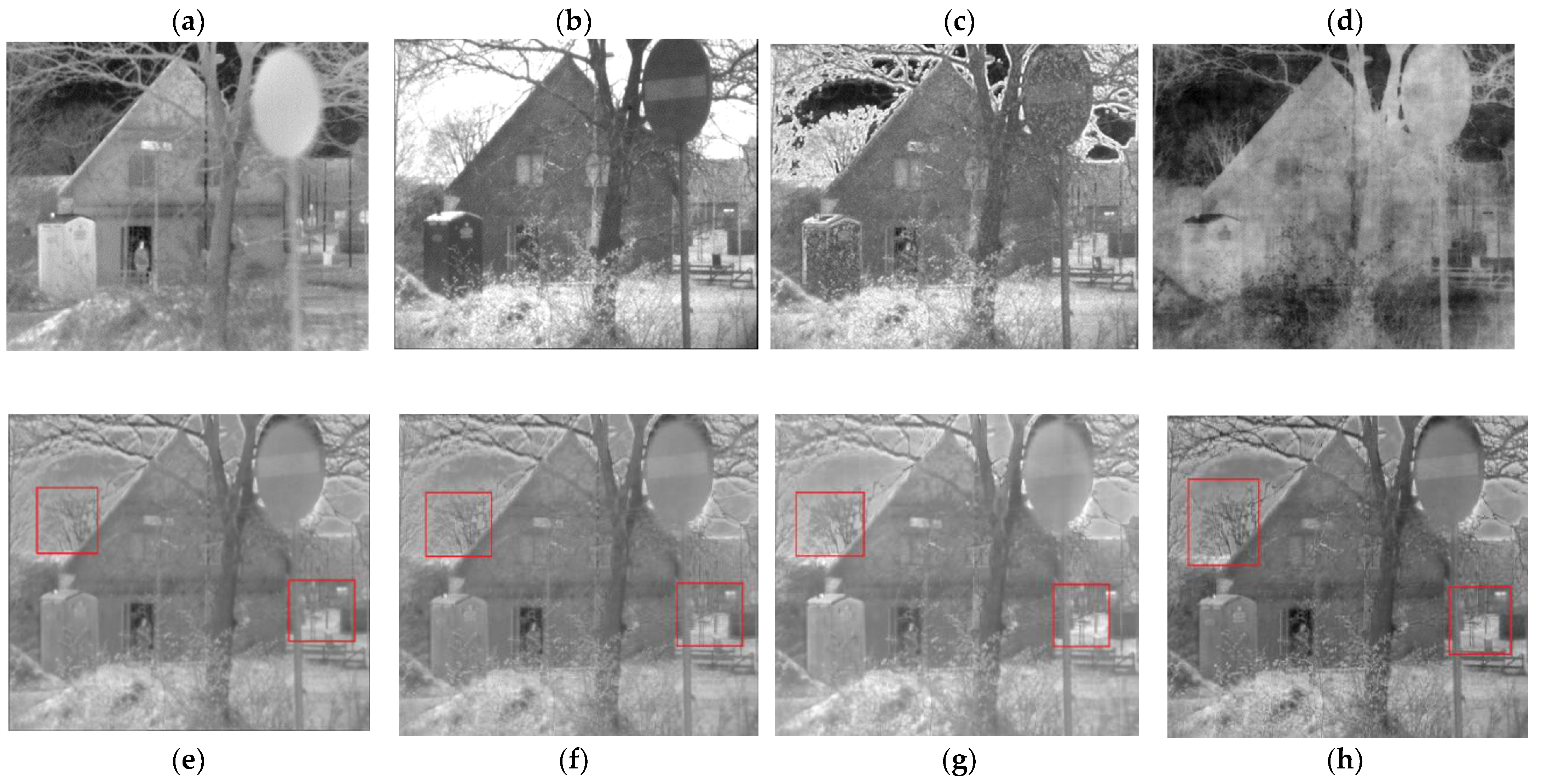
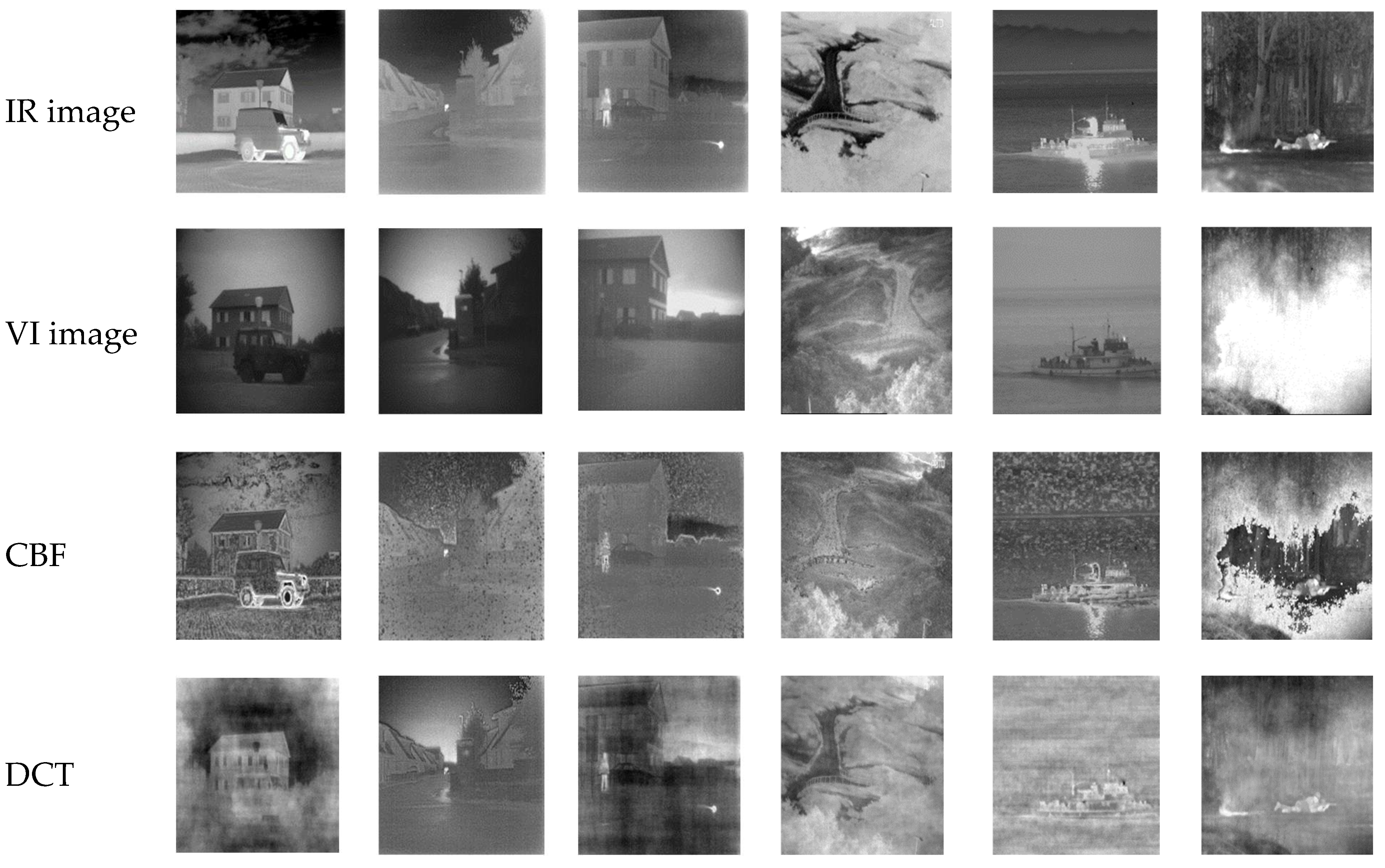
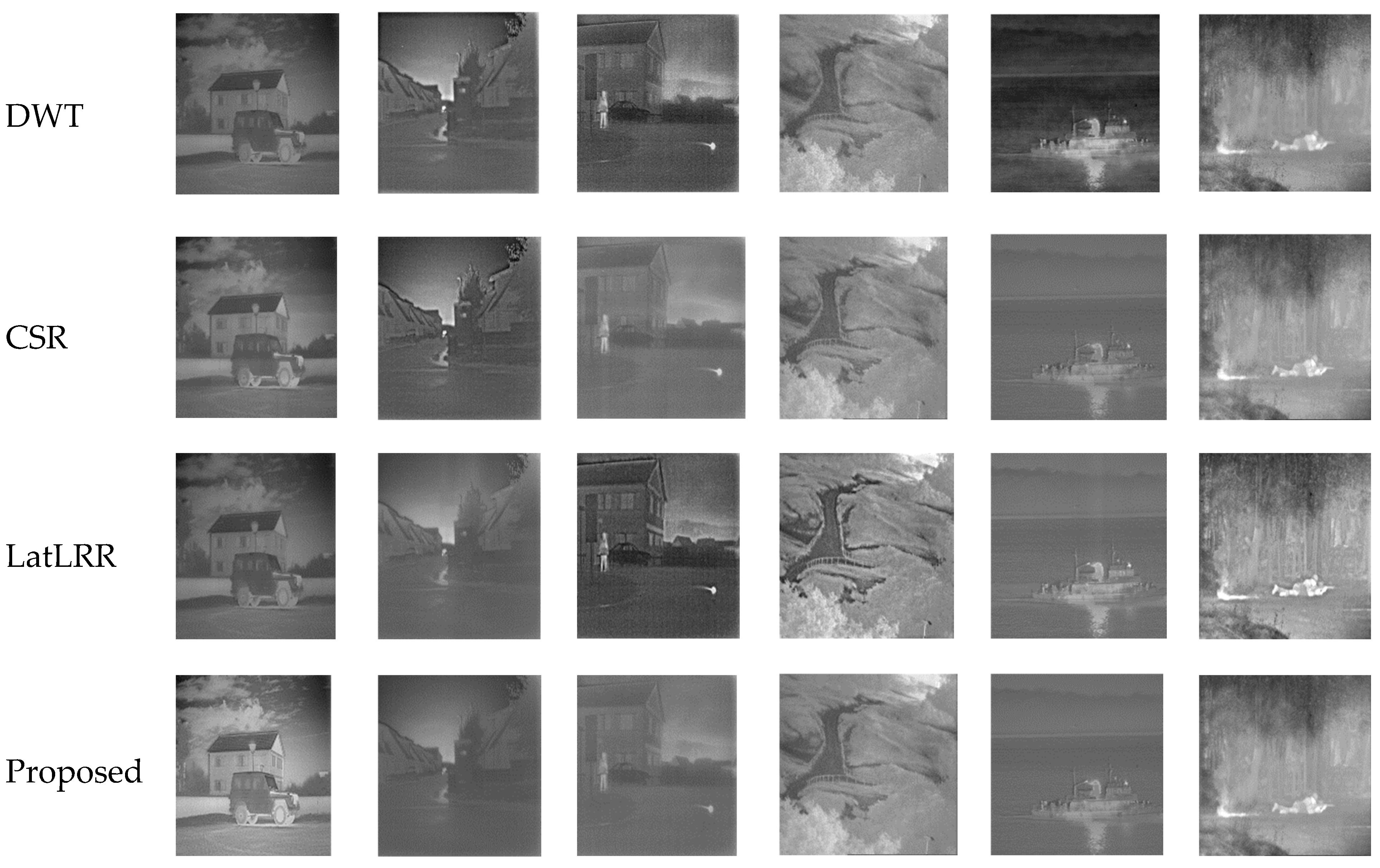
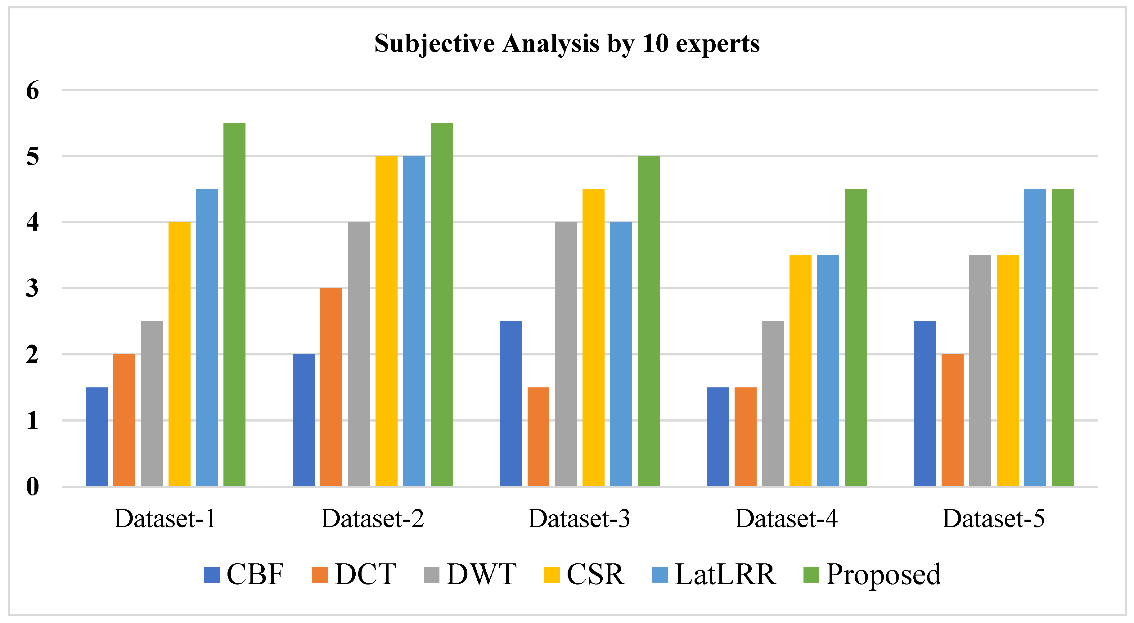
All in all, from a visual perspective, it can be observed from Figure 6, Figure 7, Figure 8, Figure 9, Figure 10 and Figure 11, and experts ranking in Table 2 and 
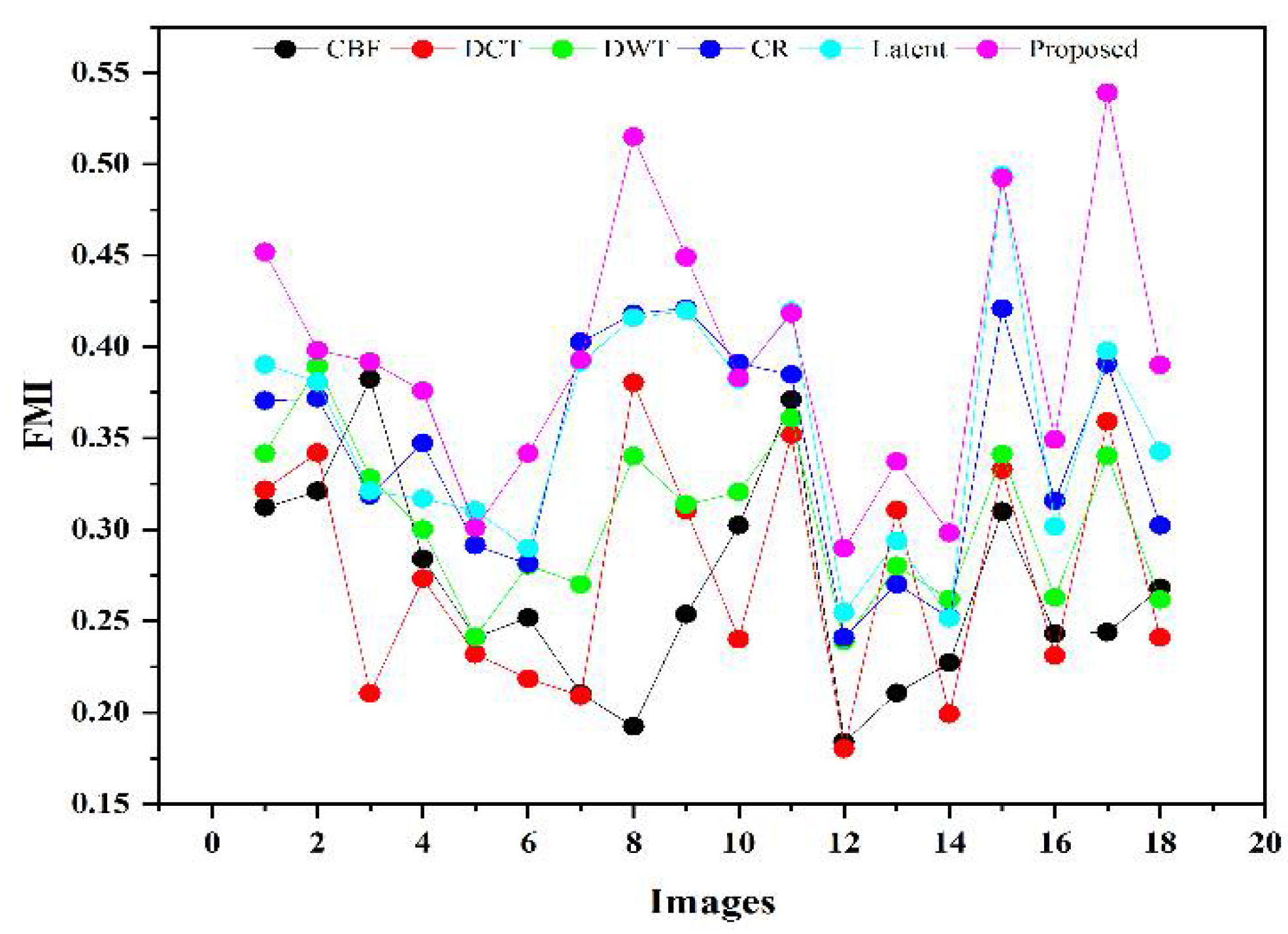
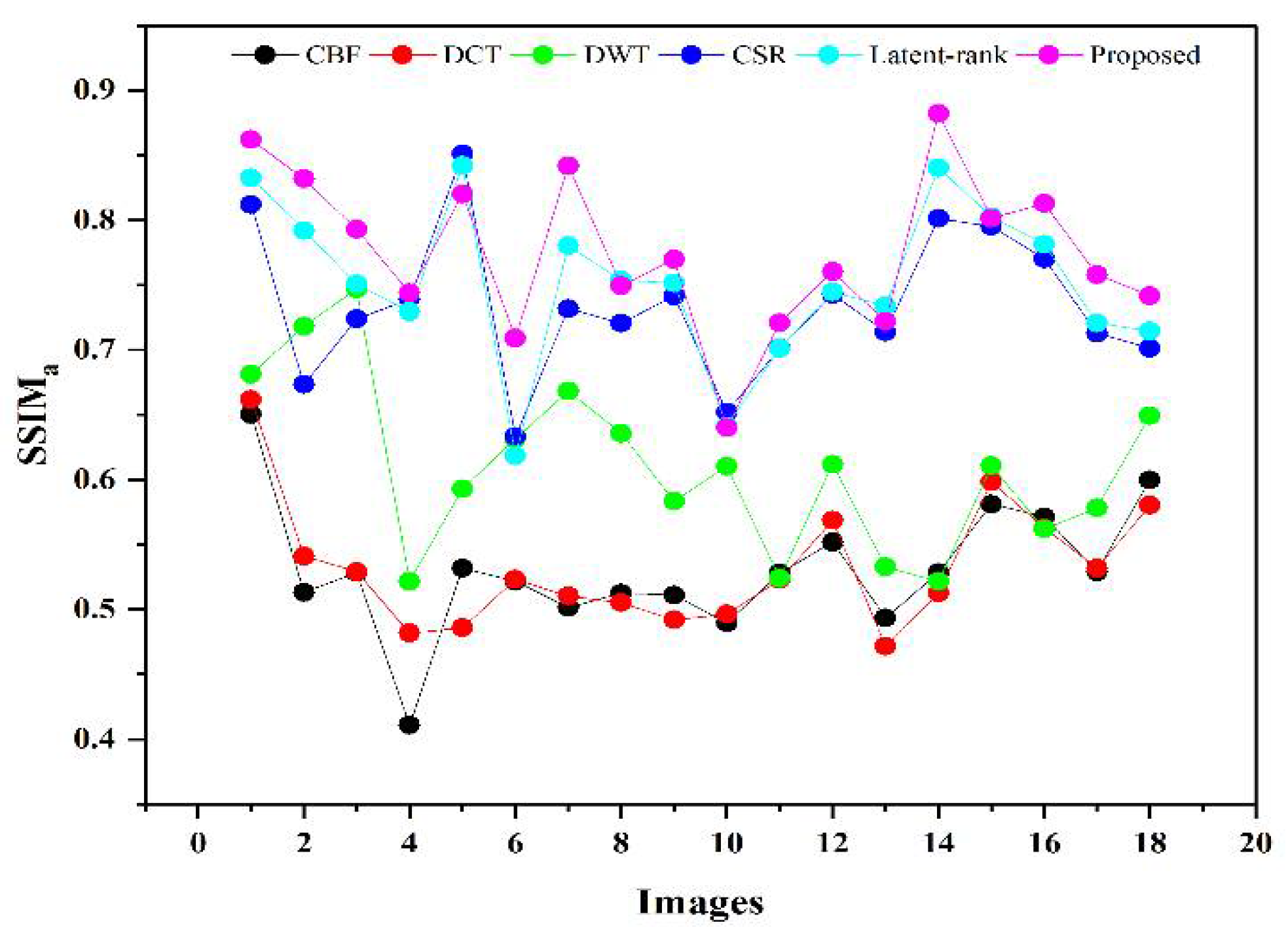
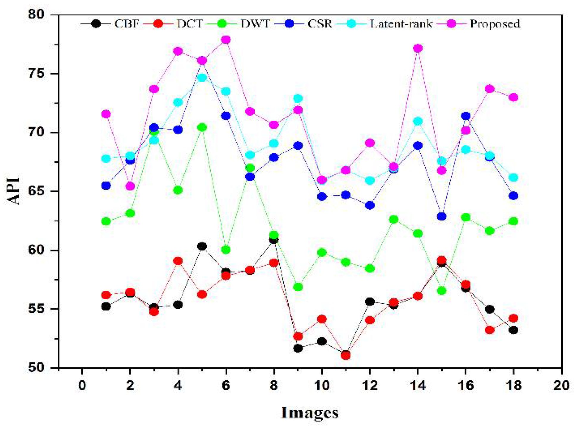
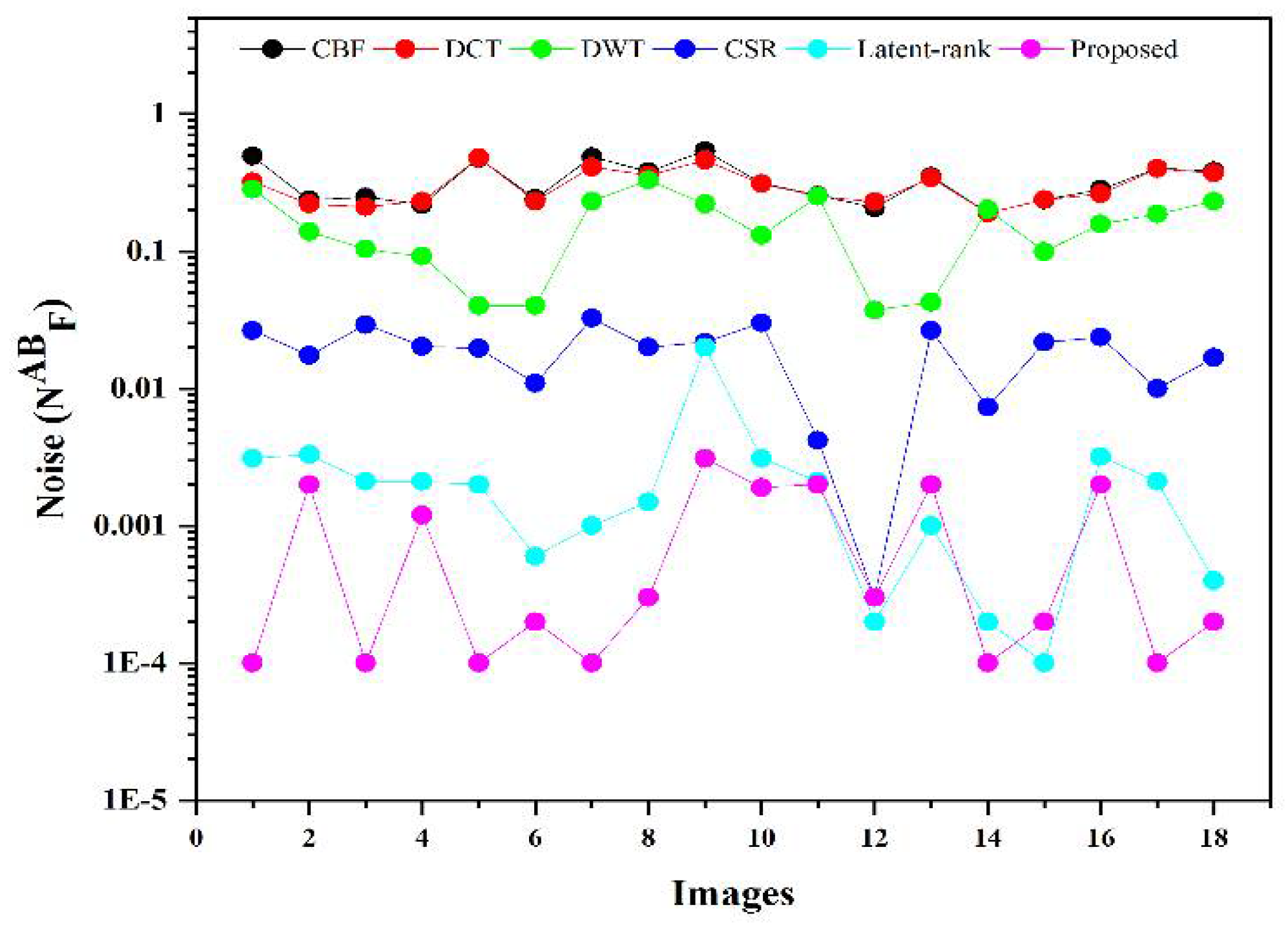
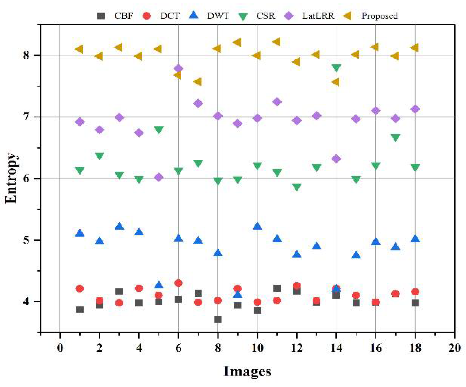
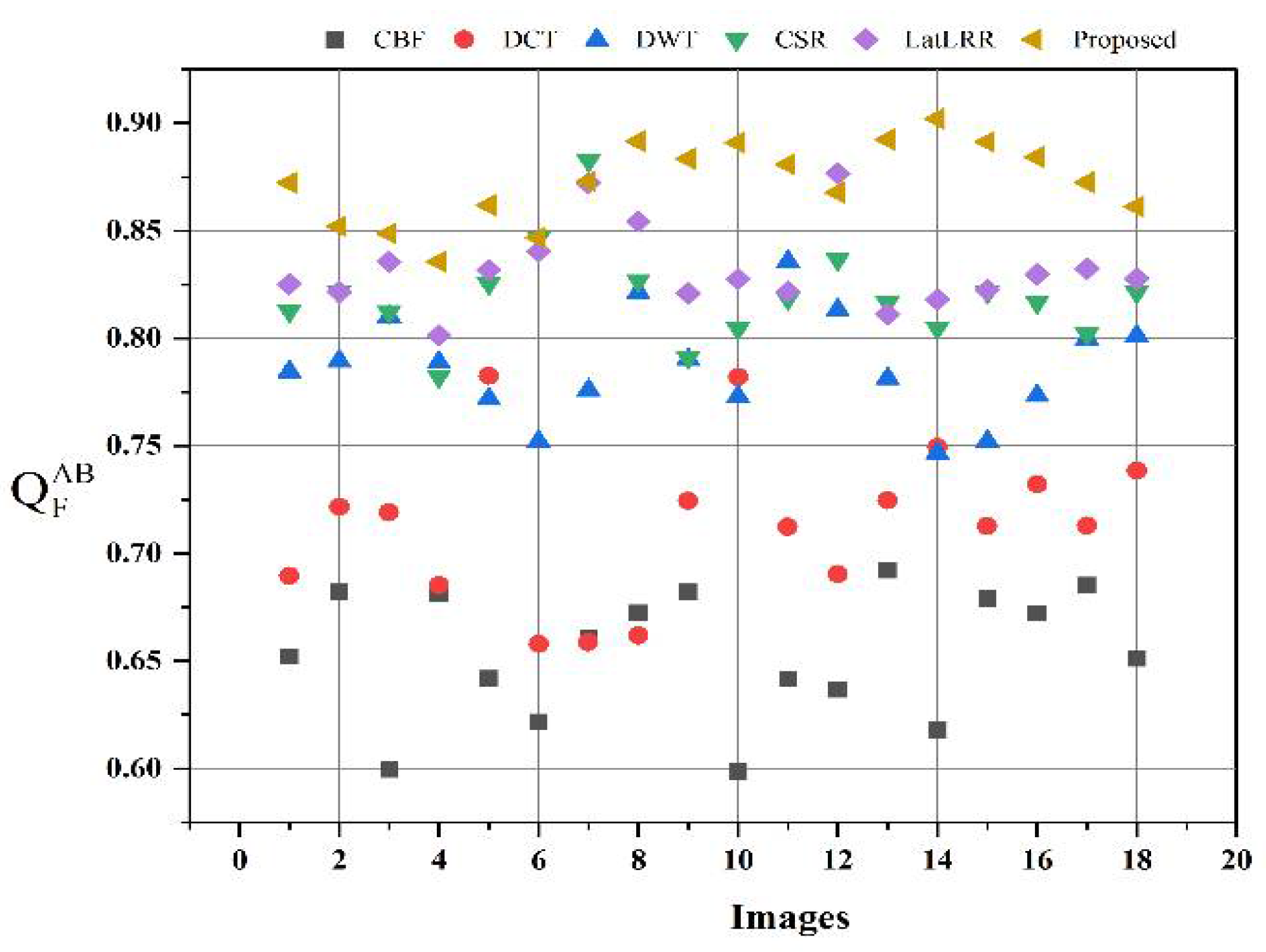
Figure 12, that the proposed method produced a better quality fused image than the other fusion methods, demonstrating the supremacy of our method. Similarly, the proposed method has better values in the indexes of F M I , S S I M a , A P I , EN, Q F A B , and N F A B objective evaluation assessment that further justify the dominancy of the proposed work.
Although the proposed work shows supremacy over recent fusion methods, this work still has limitations. The proposed work is implemented for the general IR and VI image fusion framework. However, the IR and VI image fusion for a specific application needs particular details based on that application. Therefore, we will extend this work for specific applications such as night vision and surveillance. The computation time of the proposed method is not very favorable. In future research, we will emphasize reducing the consumption time while sustaining the improved quality of a fused image.

5. Conclusions

A novel IR and VI image fusion method is proposed in this work. This work contains several stages of novel techniques. We use fuzzy set-based contrast enhancement to automatically adjust the contrast of images with its adaptive calculation and an anisotropic diffusion to remove noise from smooth regions while capturing sharp edges. Moreover, a deep learning network based on four convolutional layers named VGG-19 through transfer learning is exploited to detail images to restore substantial features. Concurrently, it saves time and resources during training and restores spectral information. The extracted detailed features are fed into L 1 n o r m and the averaging fusion scheme with a max selection rule that helps to remove the noise in smooth regions, thereby resulting in sharp edges. The PCA method is applied to base parts to preserve the essential energy information by eliminating the redundant information with its robust operation. Finally, a fused image is obtained by the superposition of base and detail parts containing substantial rich and detailed features with negligible noise. The proposed method is compared with other methods on subjective and objective assessments. The subjective analysis is performed by statistical tests (Wilcoxon signed-rank and Friedman) and experts’ visual experience. In contrast, the objective evaluation is conducted by computing the quality parameters (FMI, S S I M a , API, EN, Q F A B , and N F A B ). The proposed method exhibits superiority by obtaining a smaller value for statistical tests than other methods from a subjective perspective. Besides, experts also prefer the average results produced by the proposed method. In addition, the proposed method further justifies its efficacy for objective parameters by achieving 0.2651 to 0.3951, 0.5827 to 0.8469, 56.3710 to 71.9081, 4.0117 to 7.9907, 0.6538 to 0.8727 gain for F M I , S S I M a , A P I , E N , and Q F A B respectively
Intuitively, it can be concluded that the proposed method achieves optimal fusion performance. Our next research direction is to implement a framework for other image fusion tasks such as multimodal remote sensing, medical imaging, and multi-focus. In addition, we can apply transfer learning to other deep convolutional networks in image fusion to improve the fusion quality.

Author Contributions

Conceptualization, J.A.B.; Data curation, J.A.B.; Funding acquisition, L.T.; Methodology, J.A.B.; Resources, L.T. and Q.D.; Software, Z.S.; Supervision, L.T. and Q.D.; Validation, L.Y.; Writing—review & editing, T.A.S. All authors have read and agreed to the published version of the manuscript.

Funding

This research study is funded by: Key-Area Research and Development Program of Guangdong Province (2018B010109001), Key-Area Research and Development Program of Guangdong Province (No. 2020B1111010002), Key-Area Research and Development Program of Guangdong Province (2019B020214001), and Guangdong Marine Economic Development Project (GDNRC (2020)018).

Institutional Review Board Statement

Not applicable.

Informed Consent Statement

Not available.

Data Availability Statement

This study didn’t report data.

Conflicts of Interest

The authors claim no conflict of interest in the present research work.

References

  1. Zhou, H.; Hou, J.; Wu, W.; Zhang, Y.; Wu, Y.; Ma, J. Infrared and Visible Image Fusion Based on Semantic Segmentation. J. Comput. Res. Dev. 2021, 58, 436. [Google Scholar]
  2. Li, G.; Lin, Y.; Qu, X. An infrared and visible image fusion method based on multi-scale transformation and norm optimization. Inf. Fusion 2021, 71, 109–129. [Google Scholar] [CrossRef]
  3. Bhutto, J.A.; Lianfang, T.; Du, Q.; Soomro, T.A.; Lubin, Y.; Tahir, M.F. An enhanced image fusion algorithm by combined histogram equalization and fast gray level grouping using multi-scale decomposition and gray-PCA. IEEE Access 2020, 8, 157005–157021. [Google Scholar] [CrossRef]
  4. Grigorev, A.; Liu, S.; Tian, Z.; Xiong, J.; Rho, S.; Feng, J. Delving deeper in drone-based person re-id by employing deep decision forest and attributes fusion. ACM Trans. Multimed. Comput. Commun. Appl. (TOMM) 2020, 16, 1–15. [Google Scholar] [CrossRef]
  5. Mallick, T.; Balaprakash, P.; Rask, E.; Macfarlane, J. Transfer learning with graph neural networks for short-term highway traffic forecasting. In Proceedings of the 2020 25th International Conference on Pattern Recognition (ICPR), Milan, Italy, 10–15 January 2021; pp. 10367–10374. [Google Scholar]
  6. Moon, J.; Kim, J.; Kang, P.; Hwang, E. Solving the cold-start problem in short-term load forecasting using tree-based methods. Energies 2020, 13, 886. [Google Scholar] [CrossRef] [Green Version]
  7. Kaur, H.; Koundal, D.; Kadyan, V. Image fusion techniques: A survey. Arch. Comput. Methods Eng. 2021, 28, 4425–4447. [Google Scholar] [CrossRef]
  8. Tawfik, N.; Elnemr, H.A.; Fakhr, M.; Dessouky, M.I.; Abd El-Samie, F.E. Survey study of multimodality medical image fusion methods. Multimed. Tools Appl. 2021, 80, 6369–6396. [Google Scholar] [CrossRef]
  9. Li, B.; Xian, Y.; Zhang, D.; Su, J.; Hu, X.; Guo, W. Multi-Sensor Image Fusion: A Survey of the State of the Art. J. Comput. Commun. 2021, 9, 73–108. [Google Scholar] [CrossRef]
  10. Zhan, L.; Zhuang, Y. Infrared and visible image fusion method based on three stages of discrete wavelet transform. Int. J. Hybrid Inf. Technol. 2016, 9, 407–418. [Google Scholar] [CrossRef]
  11. Adu, J.; Gan, J.; Wang, Y.; Huang, J. Image fusion based on nonsubsampled contourlet transform for infrared and visible light image. Infrared Phys. Technol. 2013, 61, 94–100. [Google Scholar] [CrossRef]
  12. Yang, B.; Li, S. Pixel-level image fusion with simultaneous orthogonal matching pursuit. Inf. Fusion 2012, 13, 10–19. [Google Scholar] [CrossRef]
  13. Liu, Y.; Wang, Z. Simultaneous image fusion and denoising with adaptive sparse representation. IET Image Process. 2015, 9, 347–357. [Google Scholar] [CrossRef] [Green Version]
  14. Yan, X.; Qin, H.; Li, J.; Zhou, H.; Zong, J.-g.; Zeng, Q. Infrared and visible image fusion using multiscale directional nonlocal means filter. Appl. Opt. 2015, 54, 4299–4308. [Google Scholar] [CrossRef]
  15. Kumar, B.S. Image fusion based on pixel significance using cross bilateral filter. Signal Image Video Process. 2015, 9, 1193–1204. [Google Scholar] [CrossRef]
  16. Kong, W.; Zhang, L.; Lei, Y. Novel fusion method for visible light and infrared images based on NSST–SF–PCNN. Infrared Phys. Technol. 2014, 65, 103–112. [Google Scholar] [CrossRef]
  17. Kumar, S.S.; Muttan, S. PCA-based image fusion. In Algorithms and Technologies for Multispectral, Hyperspectral, and Ultraspectral Imagery XII; SPIE: Bellingham, WA, USA, 2006; Volume 6233. [Google Scholar]
  18. Kumar, B.S. Multifocus and multispectral image fusion based on pixel significance using discrete cosine harmonic wavelet transform. Signal Image Video Process. 2013, 7, 1125–1143. [Google Scholar] [CrossRef]
  19. Tawade, L.; Aboobacker, A.B.; Ghante, F. Image fusion based on wavelet transforms. Int. J. Bio-Sci. Bio-Technol. 2014, 6, 149–162. [Google Scholar] [CrossRef]
  20. Mane, S.; Sawant, S. Image fusion of CT/MRI using DWT, PCA methods and analog DSP processor. Int. J. Eng. Res. Appl. 2014, 4, 557–563. [Google Scholar]
  21. Pradnya, M.; Ruikar, S.D. Image fusion based on stationary wavelet transform. Int. J. Adv. Eng. Res. Stud. 2013, 2, 99–101. [Google Scholar]
  22. Asmare, M.H.; Asirvadam, V.S.; Iznita, L.; Hani, A.F.M. Image enhancement by fusion in contourlet transform. Int. J. Electr. Eng. Inform. 2010, 2, 29–42. [Google Scholar] [CrossRef]
  23. Lianfang, T.; Ahmed, J.; Qiliang, D.; Shankar, B.; Adnan, S. Multi focus image fusion using combined median and average filter based hybrid stationary wavelet transform and principal component analysis. Int. J. Adv. Comput. Sci. Appl. 2018, 9, 34–41. [Google Scholar] [CrossRef]
  24. Li, H.; Liu, L.; Huang, W.; Yue, C. An improved fusion algorithm for infrared and visible images based on multi-scale transform. Infrared Phys. Technol. 2016, 74, 28–37. [Google Scholar] [CrossRef]
  25. Kim, M.; Han, D.K.; Ko, H. Joint patch clustering-based dictionary learning for multimodal image fusion. Inf. Fusion 2016, 27, 198–214. [Google Scholar] [CrossRef]
  26. Zong, J.-J.; Qiu, T.-S. Medical image fusion based on sparse representation of classified image patches. Biomed. Signal Process. Control. 2017, 34, 195–205. [Google Scholar] [CrossRef]
  27. Liu, Y.; Chen, X.; Ward, R.K.; Wang, Z.J. Image fusion with convolutional sparse representation. IEEE Signal Process. Lett. 2016, 23, 1882–1886. [Google Scholar] [CrossRef]
  28. Li, H.; Wu, X.-J. Infrared and visible image fusion using latent low-rank representation. arXiv 2018, arXiv:1804.08992. [Google Scholar]
  29. Shen, C.-T.; Chang, F.-J.; Hung, Y.-P.; Pei, S.-C. Edge-preserving image decomposition using L1 fidelity with L0 gradient. In SIGGRAPH Asia 2012 Technical Briefs; ACM Press: New York, NY, USA, 2012; pp. 1–4. [Google Scholar]
  30. Zhou, Z.; Wang, B.; Li, S.; Dong, M. Perceptual fusion of infrared and visible images through a hybrid multi-scale decomposition with Gaussian and bilateral filters. Inf. Fusion 2016, 30, 15–26. [Google Scholar] [CrossRef]
  31. Han, Y.; Hong, B.-W. Deep learning based on fourier convolutional neural network incorporating random kernels. Electronics 2021, 10, 2004. [Google Scholar] [CrossRef]
  32. Kim, C.-I.; Cho, Y.; Jung, S.; Rew, J.; Hwang, E. Animal Sounds Classification Scheme Based on Multi-Feature Network with Mixed Datasets. KSII Trans. Internet Inf. Syst. (TIIS) 2020, 14, 3384–3398. [Google Scholar]
  33. Pinto, G.; Wang, Z.; Roy, A.; Hong, T.; Capozzoli, A. Transfer learning for smart buildings: A critical review of algorithms, applications, and future perspectives. Adv. Appl. Energy 2022, 5, 100084. [Google Scholar] [CrossRef]
  34. Liu, Y.; Chen, X.; Peng, H.; Wang, Z. Multi-focus image fusion with a deep convolutional neural network. Inf. Fusion 2017, 36, 191–207. [Google Scholar] [CrossRef]
  35. Feng, Y.; Lu, H.; Bai, J.; Cao, L.; Yin, H. Fully convolutional network-based infrared and visible image fusion. Multimed. Tools Appl. 2020, 79, 15001–15014. [Google Scholar] [CrossRef]
  36. Dogra, A.; Goyal, B.; Agrawal, S. From multi-scale decomposition to non-multi-scale decomposition methods: A comprehensive survey of image fusion techniques and its applications. IEEE Access 2017, 5, 16040–16067. [Google Scholar] [CrossRef]
  37. Ma, J.; Ma, Y.; Li, C. Infrared and visible image fusion methods and applications: A survey. Inf. Fusion 2019, 45, 153–178. [Google Scholar] [CrossRef]
  38. Liu, Y.; Chen, X.; Cheng, J.; Peng, H. A medical image fusion method based on convolutional neural networks. In Proceedings of the 2017 20th International Conference on Information Fusion (Fusion), Xi’an, China, 10–13 July 2017; pp. 1–7. [Google Scholar]
  39. Zhang, Q.; Wu, Y.N.; Zhu, S.-C. Interpretable convolutional neural networks. In Proceedings of the 2018 IEEE/CVF Conference on Computer Vision and Pattern Recognition, Salt Lake City, UT, USA, 18–23 June 2018; pp. 8827–8836. [Google Scholar]
  40. Liu, Y.; Liu, S.; Wang, Z. A general framework for image fusion based on multi-scale transform and sparse representation. Inf. Fusion 2015, 24, 147–164. [Google Scholar] [CrossRef]
  41. Soundrapandiyan, R.; PVSSR, C.M. Perceptual visualization enhancement of infrared images using fuzzy sets. In Transactions on Computational Science XXV; Springer: Berlin/Heidelberg, Germany, 2015; pp. 3–19. [Google Scholar]
  42. Perona, P.; Malik, J. Scale-space and edge detection using anisotropic diffusion. IEEE Trans. Pattern Anal. Mach. Intell. 1990, 12, 629–639. [Google Scholar] [CrossRef] [Green Version]
  43. Simonyan, K.; Zisserman, A. Very deep convolutional networks for large-scale image recognition. arXiv 2014, arXiv:1409.1556. [Google Scholar]
  44. Li, H.; Wu, X.-J. Multi-focus image fusion using dictionary learning and low-rank representation. In Proceedings of the International Conference on Image and Graphics, Shanghai, China, 13–15 September 2017; pp. 675–686. [Google Scholar]
  45. Toet, A. The TNO multiband image data collection. Data Brief 2017, 15, 249. [Google Scholar] [CrossRef]
  46. Toet, A. TNO Image Fusion Dataset. Figshare Data. 2014. Available online: https://figshare.com/articles/dataset/TNO_Image_Fusion_Dataset/1008029 (accessed on 5 January 2022).
  47. Park, S.; Moon, J.; Jung, S.; Rho, S.; Baik, S.W.; Hwang, E. A two-stage industrial load forecasting scheme for day-ahead combined cooling, heating and power scheduling. Energies 2020, 13, 443. [Google Scholar] [CrossRef] [Green Version]
  48. Zhuo, K.; HaiTao, Y.; FengJie, Z.; Yang, L.; Qi, J.; JinYu, W. Research on Multi-focal Image Fusion Based on Wavelet Transform. J. Phys. Conf. Ser. 2021, 1994, 012018. [Google Scholar] [CrossRef]
  49. Panguluri, S.K.; Mohan, L. An effective fuzzy logic and particle swarm optimization based thermal and visible-light image fusion framework using curve-let transform. Optik 2021, 243, 167529. [Google Scholar] [CrossRef]
Figure 1. Block diagram of the proposed method.
Remotesensing 14 00939 g001
Figure 2. The schematic diagram of the FSE method.
Remotesensing 14 00939 g002
Figure 3. Block diagram of anisotropic diffusion.
Remotesensing 14 00939 g003
Figure 4. Block diagram of PCA for the fusion of base layers.
Remotesensing 14 00939 g004
Figure 5. Fusion of detail layers.
Remotesensing 14 00939 g005
Figure 6. Street view: (a) IR image; (b) VI image; (c) CBF; (d) DCT; (e) improved DWT; (f) CSR; (g) LatLRR; and (h) proposed method.
Remotesensing 14 00939 g006
Figure 7. Two men and house scene: (a) IR image; (b) VI image; (c) CBF; (d) DCT; (e) improved DWT; (f) CSR; (g) LatLRR; and (h) proposed method.
Remotesensing 14 00939 g007
Figure 8. River road and bench scene: (a) IR image; (b) VI image; (c) CBF; (d) DCT; (e) improved DWT; (f) CSR; (g) LatLRR; and (h) proposed method.
Remotesensing 14 00939 g008
Figure 9. Umbrella man and hut scene: (a) IR image; (b) VI image; (c) CBF; (d) DCT; (e) improved DWT; (f) CSR; (g) LatLRR; and (h) proposed method.
Remotesensing 14 00939 g009
Figure 10. Man, house, and signboard scene: (a) IR image; (b) VI image; (c) CBF; (d) DCT; (e) improved DWT; (f) CSR; (g) LatLRR; and (h) proposed method.
Remotesensing 14 00939 g010
Figure 11. IR and VI input images, other fusion methods and the proposed method. From top first row to bottom 8th row indicates IR image, VI image, CBF, DCT, improved DWT, CSR, LatLRR and proposed fusion method.
Remotesensing 14 00939 g011aRemotesensing 14 00939 g011b
Figure 12. User case (average points acquired by each method on five pairs of source images).
Remotesensing 14 00939 g012
Figure 13. Plotting the FMI for 18 images.
Remotesensing 14 00939 g013
Figure 14. Plotting the S S I M a for 18 images.
Remotesensing 14 00939 g014
Figure 15. Plotting the API for 18 images.
Remotesensing 14 00939 g015
Figure 16. Plotting the N F A B for 18 images.
Remotesensing 14 00939 g016
Figure 17. Scattering plot for EN for 18 images.
Remotesensing 14 00939 g017
Figure 18. Scattering plot for Q F A B for 18 images.
Remotesensing 14 00939 g018
Table 1. Overall summarization of all methods in related work.
MethodsTransformFusion StrategyDrawback
Multi-scale decomposition (MSD)Discrete wavelet transform (DWT) [19], discrete stationary wavelet transform (DSWT) [21], discrete cosine transform (DCT) [18], contourlet transform [22], non-subsampled contourlet transform (NSCT) [11], and non-subsampled shearlet transform (NSST) [36]Averaging, window [19], choose-max, [21] weighted averaging, activity-level measurement, region based, guided filtering based [37]Fails to provide sufficient spatial information
Edge preserving-based filtering methodsCross bilateral filtering (CBF) [15], guided filtering, mean-median filtering [23], Gaussian and bilateral filtering [30], isotropic diffusion, and anisotropic diffusion [14]Choose-max [14], average gradient, local energy, and window based [34] Introduces reversal artifacts and halo effects
Sparse representation (SR) methodsOrthogonal matching pursuit (OMD) [25], joint sparsity model, over-complete dictionary (OCD) [25], and simultaneous OMD [27]Window based [19], averaging, choose-max, and the substitution of sparse coefficients [26]Limited ability in detail preservation, dimension disaster, and high sensitivity to miss-registration
Deep learning-based methodsConvolutional neural network (CNN) [38,39], VGG-19, residual network (ResNet), full convolutional networks (FCN) [35], and Siamese networkAveraging, activity-level measurement [24], normalization method, average gradient, and local similarity strategy [3]Limited ability to restore spatial information
Hybrid methodsContourlet transform with principal component analysis (PCA) [24], mean-median-based DSWT with PCA [23], morphological method with contourlet transform, NSCT with pulse code neural network (PCNN) [16], and sparse-based convolutional neural network (CSR) [27]Window, averaging, choose-max [38], normalization scheme, activity level measurement, and average gradient [40]Miss-alignment, noise is generated due to environment or fusion, and the complexity of architecture
Table 2. The results of the Wilcoxon signed-rank and Friedman tests for different methods.
MethodsWilcoxon Signed-Rank TestFriedman Test
IR-FusedVI-FusedPSNR
CBF3.80 × 10−175.68 × 10−182.63 × 10⁻¹⁶
CSR5.67 × 10−183.87 × 10⁻¹⁸
DCT3.89 × 10−183.88 × 10⁻¹⁸
DWT3.88 × 10−185.62 × 10⁻¹⁸
LatLRR3.86 × 10−185.68 × 10⁻¹⁸
Proposed3.52 × 10−183.58 × 10⁻¹⁸
Table 3. User case (average points acquired by each method on five pairs of source images).
Dataset-1CBFDCTDWTCSRLatLRRProposed
11.522.544.55.5
2234555.5
32.51.544.545
41.51.52.53.53.54.5
52.523.53.54.54.5
Table 5. The evaluation criteria for objective assessment parameters.
Quality/ParameterFMI S S I M a APIEN Q F A B N F A B
Poor<0.28<0.6<55<4<0.7>0.3
Fair0.28–0.320.60–0.7055–604–50.7–0.750.02–0.3
Good0.33–0.370.71–0.8161–655–60.75–0.80.003–0.02
Excellent>0.37>0.81>65>6>0.8<0.003
Table 6. The average computation time for proposed and other fusion methods (unit: seconds).
MethodCBFDCTImproved DWTCSRLatLRRProposed
Time 8.611.310.7259.6313.472.3
Publisher’s Note: MDPI stays neutral with regard to jurisdictional claims in published maps and institutional affiliations.

