Stability Enhancement of Wind Energy Conversion Systems Based on Optimal Superconducting Magnetic Energy Storage Systems Using the Archimedes Optimization Algorithm

Abstract

Throughout the past several years, the renewable energy contribution and particularly the contribution of wind energy to electrical grid systems increased significantly, along with the problem of keeping the systems stable. This article presents a new optimization technique entitled the Archimedes optimization algorithm (AOA) that enhances the wind energy conversion system’s stability, integrated with a superconducting magnetic energy storage (SMES) system that uses a proportional integral (PI) controller. The AOA is a modern population technique based on Archimedes’ law of physics. The SMES system has a big impact in integrating wind generators with the electrical grid by regulating the output of wind generators and strengthening the power system’s performance. In this study, the AOA was employed to determine the optimum conditions of the PI controller that regulates the charging and discharging of the SMES system. The simulation outcomes of the AOA, the genetic algorithm (GA), and particle swarm optimization (PSO) were compared to ensure the efficacy of the introduced optimization algorithm. The simulation results showed the effectiveness of the optimally controlled SMES system, using the AOA in smoothing the output power variations and increasing the stability of the system under various operating conditions.

1. Introduction

Nowadays, many electrical companies that are still using conventional fossil fuels for generating electricity are facing many challenges due to the rising awareness worldwide towards having a cleaner environment. Accordingly, the progression of integrating renewable sources in generating electricity became a necessity in recent times [1,2,3,4]. There are many available renewable energy resources for generating electricity, including wind energy, geothermal energy, solar energy, and hydro energy. Wind energy plays a prominent role in the electrical field and is now considered a rising star in generating clean electricity. According to statistics derived from the Global Wind Energy Council’s updated survey [5], the global wind-generating capacity in 2020 was around 744 GW, and 93 GW has been added to global wind generation.

A wind conversion system comprises two major components. The first component is the turbine; the second one is the generator. Regarding turbines, the variable-speed wind turbine (VSWT) is often chosen because of its many merits, the most crucial of which is the completely adaptable turbine speed with the continuously changing wind speed [6,7]. Regarding generators, the permanent magnet synchronous generator (PMSG) is often chosen due to its categorization as one of the most functional wind generators [8,9]. One of the many advantages of the PMSG is that it does not need an external excitation system; rather, it can generate power at any speed, and it is brushless, which leads to unnoticeable friction losses.

Despite the merits of the above components, we could never neglect the fact that wind energy is by nature an unpredictable source, as wind speed changes arbitrarily [10]. This continuous change in wind speed values causes undesirable fluctuations in generated power, in addition to negative effects on voltage and frequency regulation, leading to decreasing the system’s stability.

The aim of this study, in general, was to utilize the Archimedes optimization algorithm (AOA) to minimize the objective function of the system under study and at the same time not to violate the system constraints that will be explained in the following section.

More details on the problem formulation, the model, and the optimization technique will be discussed in several sections of the paper.

1.1. Low Voltage Ride through (LVRT)

Nowadays, researchers face a great challenge for solving problems related to large wind farms connected to electricity networks, including improving the performance of low voltage ride through (LVRT). LVRT stipulations indicate that even during unexpected external events such as network faults, wind generators must continue to operate normally and remain connected to the electrical network. Modern wind farm grid regulations require that wind power generators have LVRT capabilities [11].

As a result, wind power integration grid code specifications in different countries insist on including the LVRT requirements, which assure that wind farms are connected and supporting the grid during and after an unexpected fault, in addition to withstanding voltage dips limited to a certain percentage and for a specified time duration, as essential conditions for issuing a license for wind farm establishment [12,13].

The above requirements for LVRT can be encountered by two methods: integrating energy storage systems (ESS) [14,15] for wind systems, and developing optimized control techniques [16,17,18] to control the performance of an integrated ESS.

1.2. Overview of Energy Storage Systems(ESS)

Here, we discuss the first method of LVRT, which is ESS. In major grids, newly planned wind farms are frequently located in rural locations, where network capacity is generally limited, resulting in technical restrictions. In cases of excessive voltage fluctuation or thermal overloading in some of the power system components during the peak power production of a wind farm, these changes could be remedied by temporarily storing energy in an ESS and dispatching it when there is less wind. This remedy allows more wind energy to be collected than would otherwise have been the case. Simultaneously, the power electronic devices associated with an ESS can enhance power quality at a wind farm’s point of connection and assist in achieving compliance with various grid code requirements, such as voltage regulation, LVRT capabilities, and flicker reduction.

Nowadays, there are many types of ESS, including battery energy storage (BESS) [19], flywheel storage [20], fuel cell storage [21], superconducting magnetic energy storage (SMES) [22,23], compressed air energy storage (CAES) [24], and compressed carbon dioxide energy storage (CCES) [25], which are commonly utilized to resolve the drawbacks of wind energy conversion systems.

The combination of three essential elements (no-restrict-loss current, magnetic fields, and energy storage in a magnetic field) in a superconducting coil opens up the possibility of very efficient electrical energy storage. The SMES system differs from other storage methods in that the stored energy is produced by a constantly circulating current within the superconducting coil. Furthermore, the SMES system’s only conversion procedure is from AC to DC. As a result, there are no intrinsic thermodynamic losses associated with energy conversion from one type to another.

Recently, the SMES system’s application in different power systems has received much interest, due to great breakthroughs in the power electronics development field. SMES systems now haves many applications in the fields of distributed energy storage, transient stability, power quality enhancement, spinning reserve, and voltage control. Recently, there has been widespread use of SMES in several power systems, due to its several strengths, including:

• A large storage capacity that can reach, in some cases, more than 90% of rated capacity;
• Rapid charging and discharging capabilities that enhance the system’s response time; and
• Greater reliability, as it has no rotating parts and is environmentally friendly.

Despite the various merits of SMES systems, they have several disadvantages, including:

• High cooling demand;
• Complicated design;
• Temperature sensitivity;
• Expensive raw materials; and
• High costs in operation, making them economical only in short cyclic periods.

However, due to the continuous research and development in the field of power electronics and control strategies, it is expected that the relatively high costs of SMES systems will decrease in the near future.

1.3. Optimized Control Tehniques

The second method of LVRT is optimized control techniques, which incorporate both an efficient and stable fast response control strategy and a good optimization technique. The control tactics can include various controller types, including proportional differential (PD) [26], proportional integral (PI) [27], and proportional integral derivative (PID) [28]. There are various control systems that avoid using PD or PID, owing to their derivative control action that raises the system’s harmonic input frequency, potentially bringing an unstable intervention into the system. This disadvantage has compelled the development of a filter that helps in eradicating the unstable intervention system’s behavior. On the other hand, PI controllers are recognized by their ruggedness and extended stability margins, which explains why they are extensively used in industrial applications.

Considering the importance and complexity of tuning the parameters of a PI controller [29,30], various optimization techniques are being employed to complete this difficult mission. Over the last few years, there has been a remarkable progression in the use and enhancement of various optimization strategies. As a result, numerous optimization algorithms are currently being tested in different electric power systems.

The numerous optimization techniques include the cuckoo search optimization [31], Harris Hawks optimization (HHO) [32], grey wolf optimization (GWO) [33], sunflower optimization (SFO) [34], salp swarm optimization (SSO) [35], the genetic algorithm (GA) [36],the tree seed algorithm [37], the krill herd algorithm (KHA) [38], the black hole algorithm (BH) [39], particle swarm optimization (PSO) [40], and the coyote optimization algorithm [41]. The majority of these optimization approaches are drawn from the behavior of animals or insects. However, given the complexity and diversity of today’s computational optimization problems, as well as the need for more functional optimization approaches, a number of metaheuristic approaches inspired by fundamental physics, chemistry, and arithmetic phenomena have been proposed.

The AOA optimization technique proposed in this study is seen as a contemporary population strategy, with a concept based on Archimedes’ law of physics [42].

The (AOA) technique suggested in this paper competes with the most recent and cutting-edge optimization algorithms, as well as with other physics-inspired methods. It is important to note that the applied technique strikes a balance between exploration and exploitation. Because the AOA retains a population of solutions and examines a vast region to identify an optimum global solution, it is well suited for handling complicated optimization problems, with numerous local optimal solutions. In addition, when dealing with complex optimization issues, the AOA has a faster convergence time and achieves more reliable outcomes. Meanwhile, when dealing with comprehensive optimization issues, the AOA has a low running time, a proven ability to fetch a near-global solution in a short time, and a great search capacity.

1.4. Paper Overview

This paper provides a modern optimization tactic, the Archimedes optimization algorithm (AOA), which is used to enhance the LVRT capabilities of VSWT-PMSG systems using AOA-PI control located in an SMES unit. To the fullest extent of our knowledge, the suggested Archimedes tactic has not yet been documented in the literature related to enhancing the LVRT performance of wind farms.

The remaining part of this paper includes the following: Section 2 depicts the comprehensive model of the system under study; Section 3 presents a detailed explanation of the utilized optimization techniques, along with their related theoretical concepts and mathematical equations; Section 4 presents an explanation for the application of the optimization technique to the system and how it works in order to reach the optimal solution; Section 5 features the case study simulation results; and Section 6 summarizes the paper’s conclusions and provides recommendations for the future.

We would like to emphasize the important contributions of this research:

➢

We present the Archimedes optimization algorithm (AOA), a novel population-based method that resembles the Archimedes principle;

➢

The statistical significance, convergence capability, exploitation-exploration ratio, and variety of AOA solutions are all assessed;

➢

To assess the impact of the proposed approach, a series of simulations using MATLAB were conducted. These simulation experiments were carried out utilizing real-world wind data to validate the performance of the AOA-PI system; and

➢

The reliability of the optimized PI controllers employing the AOA algorithm is evaluated by contrasting its results with the results of optimized PI controllers employing the GA and PSO algorithms under various operating circumstances.

2. Power System Mathematical Modelling

2.1. Overview of the System under Study

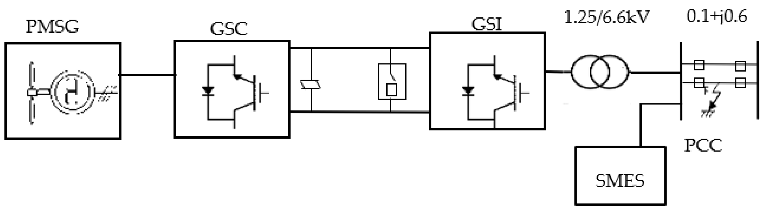
The system under study in this article comprises a VSWT and a PMSG tied to the network via a frequency converter (FC). The FC is comprised of a generator side converter (GSC), a grid side inverter (GSI) and a DC link capacitor (C_DC). With respect to the unit’s power factor value, the GSC has the capability to acquire the wind system’s maximum active power. The key function of the GSI is to control the DC link voltage, in addition to the terminal voltage. An overvoltage protection system (OVPS) is utilized to guard the C_DC.

To connect the SMES system to any power system, there should be an additional stage of power conversion, which is considered as an additional cost. However, the advantages of the system under study include a DC link capacitor (C_DC) that can be utilized to connect the SMES system without any additional expenses. The wind system model under study is described in Figure 1. The model comprises a VSWT coupled with a PMSG, a GSC, an SMES unit, a DC capacitor, an OVPS, and a GSI.

A step-up transformer and a dual circuit transmission line are utilized to connect the system under study to the electrical network. The SMES system is linked to the wind system model at the point of common coupling (PCC).

2.2. Wind Turbine and PMSG Mathematical Model

The mechanical power and speed mathematical relations [7,8,9,23] are expressed by Equations (1)–(4)$:$

$${\mathrm{P}}_{\mathsf{\omega }}^{ }=0.5{ \mathsf{\rho } \mathsf{\pi } \mathrm{R}}^{ 2}{\mathrm{V}}_{\mathsf{\omega }}^{3 }{\mathrm{C}}_{\mathrm{P}}\left(\mathsf{\lambda },\mathsf{\beta }\right)$$

(1)

$$\mathsf{\lambda } = \frac{{\mathsf{\omega }}_{\mathrm{r}} \mathrm{R}}{{\mathrm{V}}_{\mathsf{\omega }}}$$

(2)

$${\mathrm{L}}_{\mathrm{i}}=\frac{1}{\left(\frac{1}{1+0.02\mathsf{\beta }}\right)-\left(\frac{0.03}{\mathsf{\beta }3+1}\right)}$$

(3)

$${\mathrm{C}}_{\mathrm{P}}\left(\mathsf{\lambda } , \mathsf{\beta }\right)=0.73\left(\left(\frac{151}{{\mathrm{L}}_{\mathrm{i}}}\right)-0.58\mathsf{\beta }-0.002 \left({\mathsf{\beta }}^{2.14}\right)-13.2\right){\mathrm{e}}^{-\frac{18.4}{{\mathsf{\lambda }}_{\mathrm{i}}}}$$

(4)

where ${\mathrm{P}}_{\mathsf{\omega }}^{ }$ is the wind power, $\mathsf{\rho }$ is the air density, R is the blade radius, ${\mathrm{V}}_{\mathsf{\omega }}^{ }$ is the wind speed, ${\mathrm{C}}_{\mathrm{P}}$ is the power coefficient, λ is the tip speed ratio, $\mathsf{\beta }$ is the turbine pitch angle, and ${\mathsf{\omega }}_{\mathrm{r}}^{ }$ is the rotor rotational speed.

One of the significant benefits of a VSWT is the capacity to adjust the system speed with the wind speed, as well as its capability, at the same time, to derive maximum power (${\mathrm{P}}_{\max }^{ }$). This benefit is known as maximum power point tracking (MPPT).

The ${\mathrm{P}}_{\max }^{ }$ and ${\mathsf{\omega }}_{\mathrm{r}}^{ }$ mathematical equation is explained in Equation (5):

$${\mathrm{P}}_{\max }=0.5{ \mathsf{\rho } \mathsf{\pi } \mathrm{R}}^{2 }{\left(\frac{{\mathsf{\omega }}_{\mathrm{r}} \mathrm{R}}{{\mathsf{\lambda }}_{\mathrm{opt}}}\right)}^3{ \mathrm{C}}_{\mathrm{P}\text{-}\mathrm{opt}}$$

(5)

where ${\mathrm{P}}_{\max }$ is the maximum power, ${\mathrm{C}}_{\mathrm{P}\text{-}\mathrm{opt}}$ is the optimum power coefficient, and ${\mathsf{\lambda }}_{\mathrm{opt}}$ is the optimum value of the ratio of the tip speed.

In order to calculate the voltage mathematical relations in the d-q axis, Equations (6)–(8) were used as follows:

$${\mathrm{V}}_{\mathrm{ds}}={ \mathrm{R}}_{\mathrm{s}}{ \mathrm{i}}_{\mathrm{ds} }+{ \mathrm{L}}_{\mathrm{d} }\left(\frac{{\mathrm{di} }_{\mathrm{ds}}}{\mathrm{dt}}\right)-{ \mathsf{\omega }}_{\mathrm{e} }{ \mathrm{L}}_{\mathrm{q} }{ \mathrm{i}}_{\mathrm{qs} }$$

(6)

$${\mathrm{V}}_{\mathrm{qs}}={ \mathrm{R}}_{\mathrm{s}}{ \mathrm{i}}_{\mathrm{qs} }+{ \mathrm{L}}_{\mathrm{q} }\left(\frac{{\mathrm{di} }_{\mathrm{qs}}}{\mathrm{dt}}\right)+{ \mathsf{\omega }}_{\mathrm{e} }{\mathsf{\lambda }}_{\mathrm{m}}+{ \mathsf{\omega }}_{\mathrm{e} }{ \mathrm{L}}_{\mathrm{d} }{\mathrm{i}}_{\mathrm{ds} }$$

(7)

$${\mathsf{\omega }}_{\mathrm{e} }={ \mathrm{P} \mathsf{\omega }}_{\mathrm{r} }$$

(8)

where ${\mathrm{V}}_{\mathrm{ds}}$ is the stator voltage in the d-axis,${ \mathrm{R}}_{\mathrm{s}}$ is the stator resistance, ${\mathrm{i}}_{\mathrm{ds}}$ is the stator current in the d-axis, ${\mathrm{L}}_{\mathrm{d}}$ is the stator inductance in the d-axis,${ \mathsf{\lambda }}_{\mathrm{m}}$ is the magnetic flux of the PMS, ${\mathrm{V}}_{\mathrm{qs}}$ is the stator voltage in the q-axis,${ \mathrm{i}}_{\mathrm{qs}}$ is the stator current in the q-axis, ${\mathrm{L}}_{\mathrm{q}}$ is the stator inductance in the q-axis, ${\mathsf{\omega }}_{\mathrm{e}}$ is the electrical angular speed, and P is the pole pair number of the PMSG.

The PMSG mechanical dynamics, including torque, active and reactive power, are represented in Equations (9)–(12):

$$\mathrm{J} \left( \frac{{\mathrm{d}\mathsf{\omega }}_{\mathrm{r} }}{\mathrm{dt}} \right)+{\mathrm{D} \mathsf{\omega }}_{\mathrm{r} }={\mathrm{T}}_{\mathrm{m} }-{ \mathrm{T}}_{\mathrm{e} }$$

(9)

$${\mathrm{T}}_{\mathrm{e} }=\frac{3}{2} \mathrm{P} \left[\left({ \mathrm{L}}_{\mathrm{d} }-{\mathrm{L}}_{\mathrm{q} }\right){ \mathrm{i}}_{\mathrm{ds} }{\mathrm{i}}_{\mathrm{qs} }-{\mathsf{\lambda }}_{\mathrm{m}}{ \mathrm{i}}_{\mathrm{qs} } \right]$$

(10)

$${\mathrm{P}}_{\mathrm{pmsg} }=\frac{3}{2}\left[{\mathrm{v}}_{\mathrm{sd} }{\mathrm{i}}_{\mathrm{sd} }+{ \mathrm{v}}_{\mathrm{sq} }{\mathrm{i}}_{\mathrm{sq} }\right]$$

(11)

$${\mathrm{Q}}_{\mathrm{pmsg} }=\frac{3}{2}\left[{\mathrm{v}}_{\mathrm{sq} }{\mathrm{i}}_{\mathrm{sq} }+{ \mathrm{v}}_{\mathrm{sd} }{\mathrm{i}}_{\mathrm{sd} }\right]$$

(12)

where J is the moment of inertia of PMSG, D is the generator rotor damping coefficient, ${\mathrm{T}}_{\mathrm{e} }$ is the electromagnetic torque of PMSG, ${\mathrm{T}}_{\mathrm{m}}$ is the mechanical torque of PMSG, ${\mathrm{P}}_{\mathrm{pmsg}}$ is the real power of the PMSG, and ${\mathrm{Q}}_{\mathrm{pmsg}}$ is the reactive power of the PMSG.

2.3. SMES Mathematical Model

When constructing a SMES system, good design is extremely important and many authors have presented innovative solutions [43,44]. The optimization of dimensions, while keeping an appropriate constraint of the parameters in mind, aids in the improvement of such a design. There are various fascinating computer tools for optimization (e.g., MS Excel or MATLAB) that offer particular solutions for this work, but the mathematical description of the issue is the key to success in all circumstances. There are two primary configurations employed for SMES system design (solenoidal and toroidal configurations), which have already been studied from various perspectives [45].

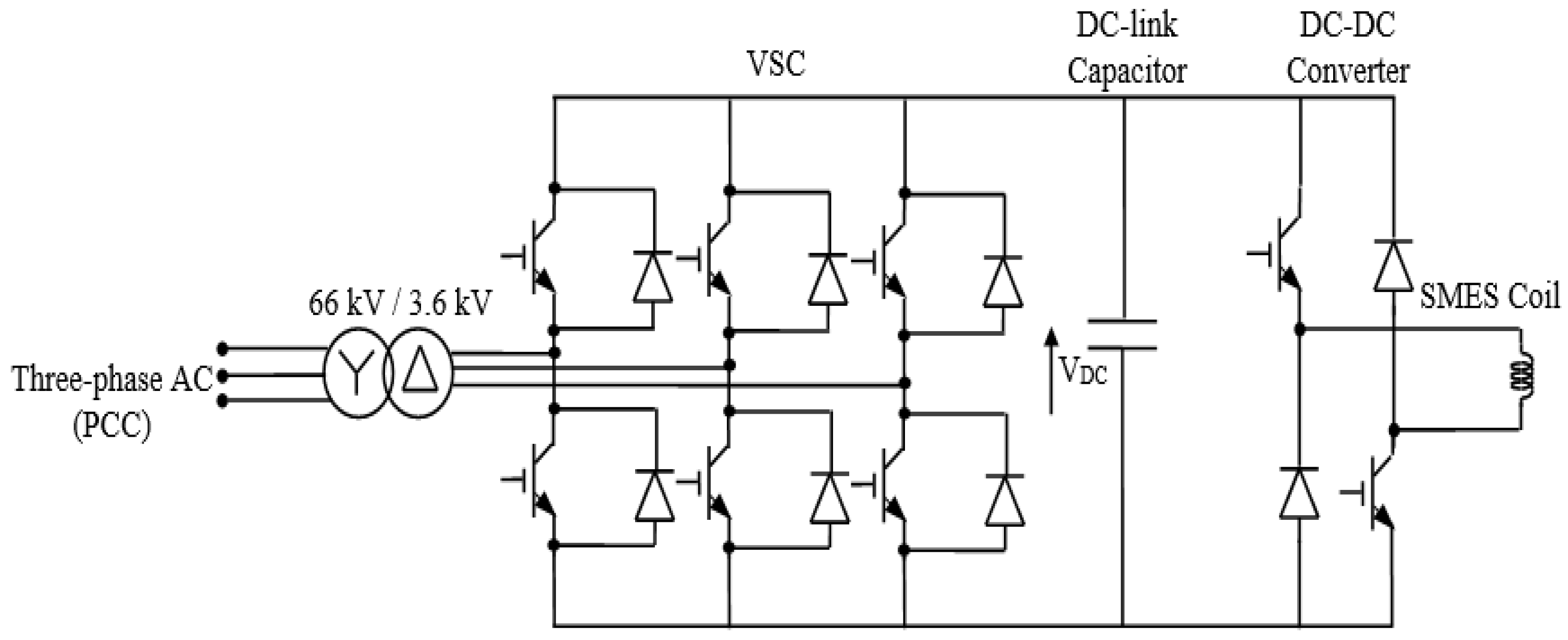
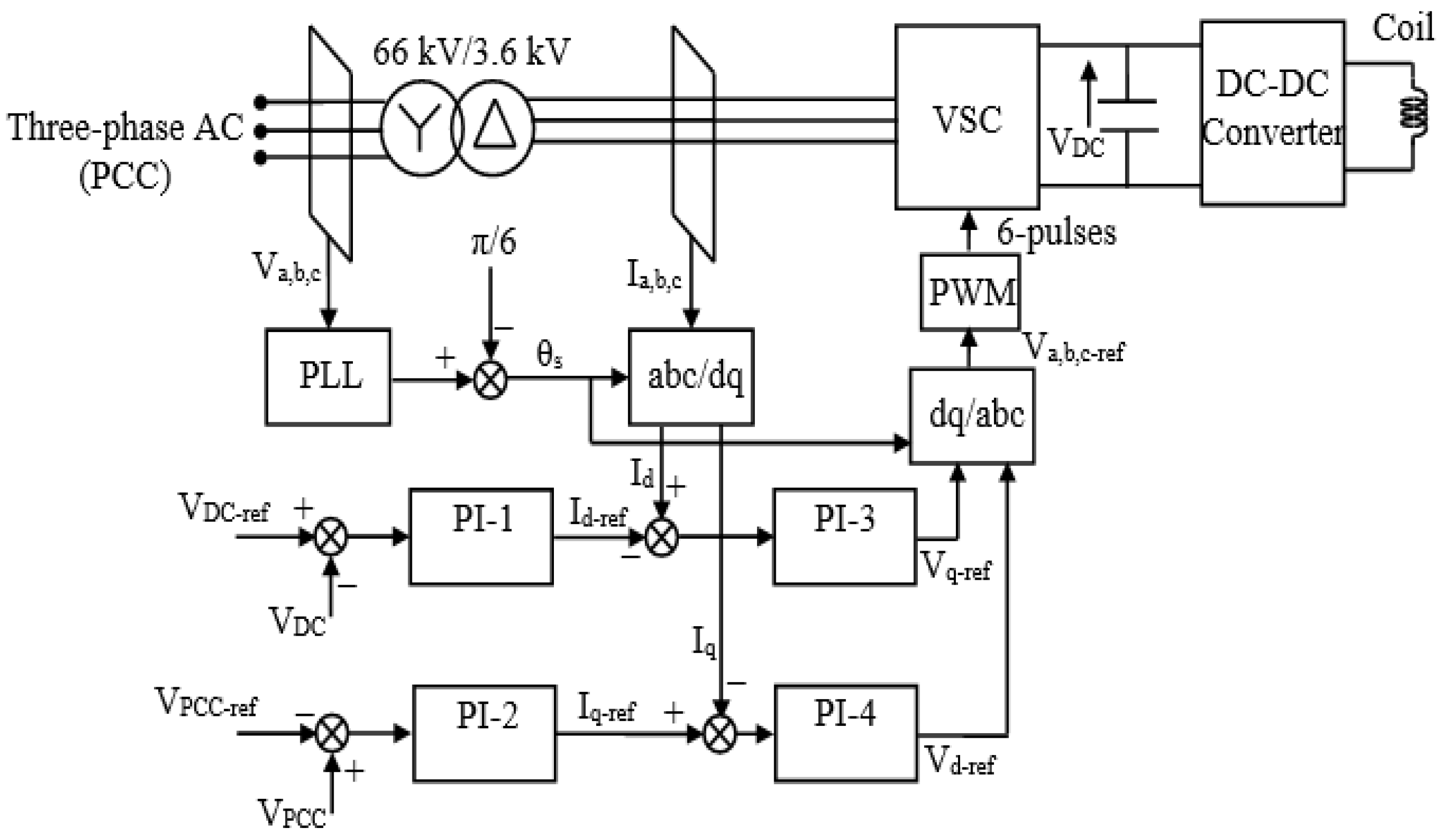
In this article, the proposed SMES system model utilized under study comprises a three-phase star delta transformer, a voltage source converter (VSC) with a six–pulses, pulse-width modulation (PWM) utilizing insulated gate bipolar transistors (IGBTs), a DC link capacitor with 60 mF, a DC-DC two-quadrant chopper utilizing IGBTs, and a super conducting coil with an inductance value of 0.24 H. The model is shown in Figure 2. The mathematical equations of the SMES system’s energy (E) and power (P) [25,43,44], are explained by Equations (13) and (14):

$$\mathrm{E}=0.5{ \mathrm{L}}_{\mathrm{sm}}{ \mathrm{I}}_{\mathrm{sm}}^2$$

(13)

$$\mathrm{P}=\frac{\mathrm{dE}}{\mathrm{dt}}={\mathrm{L}}_{\mathrm{sm} }{\mathrm{I}}_{\mathrm{sm} }\frac{{\mathrm{dI}}_{\mathrm{sm} }}{\mathrm{dt}}={\mathrm{V}}_{\mathrm{sm} }{\mathrm{I}}_{\mathrm{sm} }$$

(14)

where ${\mathrm{L}}_{\mathrm{sm}}$ is the superconducting coil inductance, ${\mathrm{I}}_{\mathrm{sm}}$ is the superconducting coil current, and ${\mathrm{V}}_{\mathrm{sm}}$ is the superconducting voltage coil.

2.3.1. VSC with a Six-Pulse Pulse Width Modulation (PWM)

The voltage source converter (VSC) is a three-phase power electronic rectifier/inverter scheme that integrates the superconducting coil with the system under study through the three-phase star delta transformer. The VSC system is managed by a widely acknowledged cascaded PI controller scheme consisting of a PI-1 outer loop and a PI-2 inner loop, as illustrated in Figure 3.

In the proposed control scheme, the reference frame transformation method links all the electrical quantities (d-q) to their related three-phase electrical quantities. The phase-locked loop (PLL) technique was utilized to calculate the transformation angles of three-phase voltages (${\mathrm{V}}_{\mathrm{a} }$, ${\mathrm{V}}_{\mathrm{b} }$, ${\mathrm{V}}_{\mathrm{c}}$) at the transformer’s high voltage side. The prime objective of inserting the VSC into the SMES model was to govern the PCC and the DC link voltages.

The PI-1 controller’s inputs are the ${\mathrm{V}}_{\mathrm{DC}}$ and the ${\mathrm{V}}_{\mathrm{PCC}}$ error signals. The ${\mathrm{V}}_{\mathrm{DC}}$ error signal equals the difference between the ${\mathrm{V}}_{\mathrm{DC}}$ reference value and ${\mathrm{V}}_{\mathrm{DC}}$ real value, taking into considering the vector control technique. Furthermore, the ${\mathrm{V}}_{\mathrm{PCC}}$ error signal equals the difference between the reference value of ${\mathrm{V}}_{\mathrm{PCC}}$ and the real value of ${\mathrm{V}}_{\mathrm{PCC}}, \mathrm{while} \mathrm{also}$ considering the vector control technique. The above PI-1 controller input signals produce the reference signals ${\mathrm{I}}_{\mathrm{d}-\mathrm{ref}}$ and ${\mathrm{I}}_{\mathrm{q}-\mathrm{ref}}$.

The PI-2 controller inputs are the ${\mathrm{I}}_{\mathrm{d}-}$ and ${\mathrm{I}}_{\mathrm{q}}$ error signals, which are used for generating the ${\mathrm{V}}_{\mathrm{d}-\mathrm{ref}}$ and ${\mathrm{V}}_{\mathrm{q}-\mathrm{ref}}$ signals.

For the purpose of generating the IGBT’s gate signals, the three-phase sinusoidal reference waveform ${\mathrm{V}}_{\mathrm{a},\mathrm{b},\mathrm{c}-\mathrm{ref}}$, was obtained from the ${\mathrm{V}}_{\mathrm{d}-\mathrm{ref}}$ and ${\mathrm{V}}_{\mathrm{q}-\mathrm{ref}}$ signals by using the transformation angle (${\mathsf{\theta }}_{\mathrm{r}}$), and a comparative analysis was conducted between the obtained output signal and a triangular signal with frequency equal to 1.0 kHz, which was used to calculate the proper firing angles.

2.3.2. DC-DC Two-Quadrant Chopper Utilizing IGBTs

The process of storing or transmitting the superconducting coil’s energy depends on regulating the DC voltage across the superconducting coil. This is the reason a chopper is utilized in the SMES model.

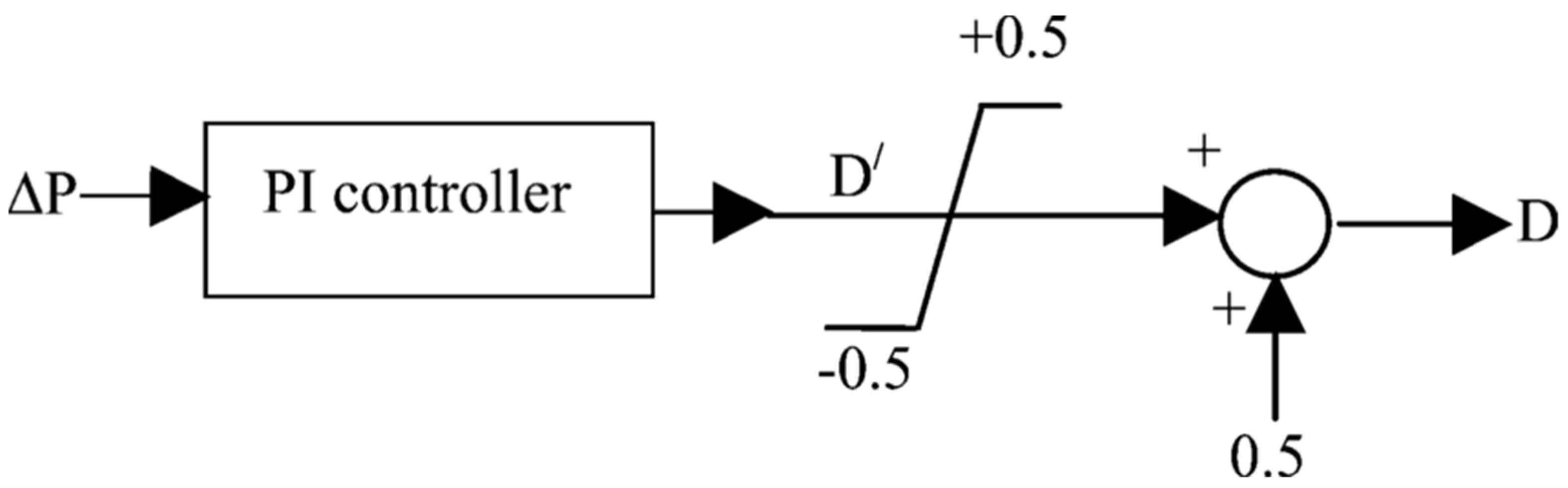
The DC-DC chopper regulates the superconducting coil’s DC voltage by fine tuning of chopper’s duty cycle. Moreover, the charging and discharging process relies on the value of the duty cycle. Once this value reaches more than 50%, the DC voltage value is positive, and the coil starts charging. On the other hand, if the duty cycle value is less than 50%, the DC voltage value is negative, and the coil starts discharging. Furthermore, for a 50% duty cycle value, the resultant DC voltage value is zero, and at this stage the coil is neither charged nor discharged. As shown in Figure 4, the input signal from the PI controller is the active power measured at the PCC error signal (ΔP), where (ΔP) is the difference between the line power value at the PCC $\left({\mathrm{P}}_{\mathrm{L}}\right)$ and the reference active power value $\left({\mathrm{P}}_{\mathrm{Lref}}\right)$. This input signal is utilized in developing the duty cycle signal (D); then, the output is compared with a triangle waveform and eventually the resulting signal is utilized to induce the gate signals for the IGBTs that are located in the DC-DC converter; the proposed triangular waveform’s frequency value is 1 kHz.

The presented case studies in this paper are concerned with optimally tuning the PI controllers by determining the optimum values of both the proportional gain (${\mathrm{K}}_{\mathrm{P}})$ and the integral time constant (${\mathrm{K}}_{\mathrm{i}}$) of the SMES system’s parameters presented in the DC-DC chopper’s duty cycle control, while at the same time demonstrating the effectiveness of the proposed controller’s optimization technique, the AOA, by comparing its results to those achieved using the GA and PSO.

Determining the optimum values of both ${\mathrm{K}}_{\mathrm{P}}$ and ${\mathrm{K}}_{\mathrm{I}}$ helps in developing the optimum value of the SMES system’s duty cycle, which is responsible for charging and discharging the SMES system’s coil, which in turn determines the value of injected active and reactive power from the SMES system into the power system.

The injected active and reactive power from the SMES system to the power system aids in maintaining the system’s stability during fault conditions, as shown and explained in the case study and simulation results section of this article.

3. System Optimization Approach, Theoretical Concepts, and Mathematical Equations

3.1. AOA Overview and Stages

3.1.1. AOA Overview

Most of the commonly used optimization techniques utilized nowadays are derived from animal or insect behaviour. However, due to the complexity and sophistication of numerical optimization problems and the need for new and effective optimization approaches, various metaheuristic approachesfrom powerful physics, chemistry, and mathematics phenomena have been introduced.

The AOA is a newly introduced population-based metaheuristic optimization tactic that is utilized to solve various optimization problems in a short duration of time [46,47,48,49,50].

The fundamental criterion of the AOA is based on Archimedes’ physical law of buoyancy. That law expresses the correlation between a body immersed in any fluid, such as water, and the buoyancy force acting on it. The law states that the buoyancy of a body exposed to an uplifting force equates to the weight of the displaced fluid where, when the weight of the body surpasses the weight of the fluid expelled, the object will sink. However, if the weight of both the object and the expelled fluid are the same, the object will float. In the AOA selected optimization technique, the members of the population were considered as objects submerged in the fluid. These population members have density, volume, and acceleration, all of which make a significant contribution to the object’s floating process. The objective of the AOA is to escalate to a point at which all of the objects of the population are equally floating, which means that the net fluid force value acting on all objects is equal to zero.

In other words, the objective of utilizing the AOA is to optimally calculate the values of ${\mathrm{K}}_{\mathrm{P}}$ and ${\mathrm{K}}_{\mathrm{i}}$ of the DC-DC chopper, where ${\mathrm{K}}_{\mathrm{P}}$ and ${\mathrm{K}}_{\mathrm{i}}$ are the design variables.

The AOA is utilized to search for the minimum of the objective function required for stability purposes, while at the same time searching for the optimum values of ${\mathrm{K}}_{\mathrm{P}}$ and ${\mathrm{K}}_{\mathrm{i}}$ that ensure the delivery of the optimum values of active and reactive power to the system and also ensure that the system operates within allowable operating limits. The objective or the fitness function is ▲P², which is required to be minimized in order to reduce system error.

$$▲\mathrm{P}=\left({\mathrm{P}}_{\mathrm{L} }-{ \mathrm{P}}_{\mathrm{Lref}}\right)$$

(15)

where ${\mathrm{P}}_{\mathrm{L}}$ is the power delivered at PCC ${\mathrm{and} \mathrm{P}}_{\mathrm{Lref}}$ is the reference power of the grid.

3.1.2. AOA Stages and Mathematical Modelling

The AOA goes through six stages until reaching a seventh stage, which is a global solution; these seven stages are thoroughly discussed in the following section [42,46,47,48]:

• Stage 1 (Initialization): In this stage, each member of the population is launched with a random position in the fluid, as illustrated in Equation (16); after that, each object’s fitness value is calculated.

  $${\mathrm{O}}_{\mathrm{i} }={\mathrm{lb}}_{\mathrm{i}}+ \mathrm{rand}\left({\mathrm{ub}}_{\mathrm{i}}-{ \mathrm{lb}}_{\mathrm{i}}\right)$$

  (16)

  $${\mathrm{Den}}_{\mathrm{i}} = \mathrm{rand}$$

  (17)

  $${\mathrm{Vol}}_{\mathrm{i}} = \mathrm{rand}$$

  (18)

  $${\mathrm{Acc}}_{\mathrm{i} }={ \mathrm{lb}}_{\mathrm{i}}+ \mathrm{rand}\left({\mathrm{ub}}_{\mathrm{i}}-{ \mathrm{lb}}_{\mathrm{i}}\right)$$

  (19)

  where ${\mathrm{O}}_{\mathrm{i}}$ is $\mathrm{i}$th object in the population, $\mathrm{is}$: search space’s lower boundary, ${\mathrm{ub}}_{\mathrm{i}}$ is the search space’s upper boundary, ${\mathrm{Den}}_{\mathrm{i}}$ is the $\mathrm{i}$th object density, rand represents a dimensional vector generates number between [0, 1] randomly, ${\mathrm{Vol}}_{\mathrm{i}}$ is the $\mathrm{i}$th object volume, and ${\mathrm{Acc}}_{\mathrm{i}}$ is the $\mathrm{i}$th object acceleration.
• Stage 2 (Update the object’s density and volume): In this stage, each object’s density and volume values are updated for an iteration t + 1, utilizing Equations (20) and (21).

  $${{\mathrm{Den}}_{\mathrm{i}}}^{\left(\mathrm{t}+1\right)}= {{\mathrm{Den}}_{\mathrm{i}}}^{\left(\mathrm{t}\right)}+\mathrm{rand} \left({\mathrm{Den}}_{\mathrm{best}} - {{\mathrm{Den}}_{\mathrm{i}}}^{\left(\mathrm{t}\right)}\right)$$

  (20)

  $${{\mathrm{Vol}}_{\mathrm{i} }}^{\left(\mathrm{t}+1\right)} = {{\mathrm{Vol}}_{\mathrm{i} }}^{\left(\mathrm{t}\right)}+ \mathrm{rand} \left({\mathrm{Vol}}_{\mathrm{best} }- {{\mathrm{Vol}}_{\mathrm{i} }}^{\left(\mathrm{t}\right)}\right)$$

  (21)

  where ${\mathrm{Den}}_{\mathrm{best}}$ is the density of the object having the best fitness, ${\mathrm{Vol}}_{\mathrm{best}}$ is the volume of the object having the best fitness.
• Stage 3 (Transfer operator and density factor): This stage witnesses the clash between the different objects inside the population. The transfer operator TF aids the transformation of the AOA search from the exploration phase to the exploitation phase, as expressed in Equation (22). The TF value steadily rises over time until approaching the unity value 1.

  $$\mathrm{TF}=\exp \left(\frac{\mathrm{t}-{\mathrm{t}}_{\max }}{{\mathrm{t}}_{\max }}\right)$$

  (22)

  where TF is the transfer operator capable of transferring the search procedure from the exploration to the exploitation stage, t is the number of iterations, ${\mathrm{t}}_{\max }$ is the maximum number of iterations. Furthermore, for the density decreasing factor (d), which is illustrated in Equation (23), its value decreases with time, which aids the AOA in discovering a close-to-global solution.

  $${\mathrm{d} }^{\left(\mathrm{t}+1\right)}= \exp \left(\frac{\mathrm{t} -{ \mathrm{t} }_{\max }}{{\mathrm{t}}_{\max }}\right)-\left(\frac{\mathrm{t}}{{\mathrm{t}}_{\max }}\right)$$

  (23)
• Stage 4 (Exploration, exploitation, and normalized acceleration phase): This stage is divided into three substages, depending on the value of the factor (TF); these substages can be illustrated as follows:

  -

  Stage 4.1 (TF ≤ 0.5):

  This substage is called Exploration, where the objects are subjected to collisions with each other; in this case, a random material (${\mathrm{m}}_{\mathrm{r}}$) is elected and the acceleration of the object is amended, as set out in Equation (24).

  $${{\mathrm{Acc}}_{\mathrm{i} }}^{\left(\mathrm{t}+1\right)}=\left(\frac{{\mathrm{Den}}_{\mathrm{mr} }+{ \mathrm{Vol}}_{\mathrm{mr} }\times { \mathrm{Acc}}_{\mathrm{mr} }}{{{\mathrm{Den}}_{\mathrm{i} }}^{\left(\mathrm{t}+1\right)} \times {{\mathrm{Vol}}_{\mathrm{i}}}^{\left(\mathrm{t}+1\right)}}\right)$$

  (24)

  where, ${\mathrm{Den}}_{\mathrm{mr}}$: is the density of the random material, ${\mathrm{Vol}}_{\mathrm{mr}}$: is the volume of the random material.

  -

  Stage 4.2 (TF $\ge$ 0.5):

  This substage is called Exploitation, where the objects are not subjected to any collisions with each other, and the object’s acceleration is amended as set out in Equation (25).

  $${{\mathrm{Acc}}_{\mathrm{i} }}^{\left(\mathrm{t}+1\right)}=\left(\frac{{\mathrm{Den}}_{\mathrm{best} }+{ \mathrm{Vol}}_{\mathrm{best} }\times { \mathrm{Acc}}_{\mathrm{best} }}{{{\mathrm{Den}}_{\mathrm{i}}}^{\left(\mathrm{t}+1\right)} \times {{\mathrm{Vol}}_{\mathrm{i}}}^{\left(\mathrm{t}+1\right)}}\right)$$

  (25)

  -

  Stage 4.3 (Normalized Acceleration)

  This substage is utilized to calculate the change’s percentage; the acceleration is illustrated as set out in Equation (26):

  $${{\mathrm{Acc}}_{\mathrm{i}\text{-}\mathrm{norm} }}^{\left(\mathrm{t}+1\right)}= \mathrm{w} \times \frac{{{\mathrm{Acc}}_{\mathrm{i} }}^{\left(\mathrm{t}+1\right)} - \min \left(\mathrm{Acc}\right)}{\max \left(\mathrm{Acc}\right)- \min \left(\mathrm{Acc}\right)}+ \mathrm{z}$$

  (26)

  where (w, z) are the normalization range that extends between 0.9 and 0.1, while ${{\mathrm{Acc}}_{\mathrm{i}\text{-}\mathrm{norm} }}^{(\mathrm{t}+1)}$ defines the proportion of each agent’s change. If the object is far from the optimal solution, the value of the acceleration will be significant, suggesting that the object is in the exploration phase; in any other situation, the object would be in the exploitation phase. This demonstrates how the search process moves from exploration to exploitation. In most cases, the acceleration factor starts with a high value and diminishes over time, which assists the search agents in moving away from local solutions and getting close to the best global solution.

• Stage 5 (Update Position): In this stage, the object is in the Exploration phase, and the position of the object is updated as per Equation (27):

  $${{\mathrm{y}}_{\mathrm{i}}}^{\left(\mathrm{t}+1\right)} = {{\mathrm{y}}_{\mathrm{i}}}^{\mathrm{t}} + {\mathrm{C}}_1 \times \mathrm{rand} \times {{\mathrm{Acc}}_{\mathrm{i}\text{-}\mathrm{norm} }}^{\left(\mathrm{t}+1\right)}\times \mathrm{d} \times \left({\mathrm{y}}_{\mathrm{rand}} - {{\mathrm{y}}_{\mathrm{i} }}^{\mathrm{t}}\right)$$

  (27)
  If the object is in the Exploitation phase, the position of the object is updated as per Equation (28):

  $${{\mathrm{y}}_{\mathrm{i}}}^{\left(\mathrm{t}+1\right)} = {{\mathrm{y}}_{\mathrm{best}}}^{\mathrm{t}}+ \mathrm{F} \times { \mathrm{C}}_{2 }\times \mathrm{rand} \times {{\mathrm{Acc}}_{\mathrm{i}\text{-}\mathrm{norm} }}^{\left(\mathrm{t}+1\right)}\times \mathrm{d} \times \left({\mathrm{T} \times \mathrm{y}}_{\mathrm{best}} - {{\mathrm{y}}_{\mathrm{i}}}^{\mathrm{t}}\right)$$

  (28)
  T increases gradually and is directly proportional to the TF factor, where T = ${\mathrm{C}}_3$ × TF.
  F is the flag to change the direction of motion:

  F = +1    if Q < 0.5

  F = −1    if Q > 0.5

  where

  $$\mathrm{Q}=2 \times \mathrm{rand} - {\mathrm{C}}_4$$
• Stage 6 (Evaluation): In this stage, the evaluation of the fitness value of each object is executed and the optimal solution is recorded together with the optimal values for ${\mathrm{y}}_{\mathrm{best} },{ \mathrm{Acc}}_{\mathrm{best} },{ \mathrm{Vol}}_{\mathrm{best} },{ \mathrm{and} \mathrm{Den}}_{\mathrm{best}}$ are assigned.

The pseudo code for the AOA [46] is presented as below (Algorithm 1):

Algorithm 1: Pseudo code of the AOA

Determine the AOA parameters; (population size (N), the maximum number of iteration (tmax), and the rand value. Initialize the objects’ population with random positions, densities, and volumes using Equations (16–18). Evaluate the initial population and select one of the best fitness values. Set t = 1. while t ≤ tmax do for each object i do Update the density and volume of each object using Equations (20) and (21). Update the transfer and density decreasing factor TF and d using Equations (22) and (23). If (TF ≤ 0.5) then     ➢ Exploration phase. Update the acceleration and normalize the acceleration using Equations (24) and (25). Update the position using Equation (27). Alternatively     ➢ Exploitation phase. Update the acceleration and normalize the acceleration using Equations (25) and (26). Update the direction flag F. Update the position using Equation (28). end if end for Evaluate each object and select the one with the best fitness value. Set t = t + 1. end while return object with the best fitness value. end procedure

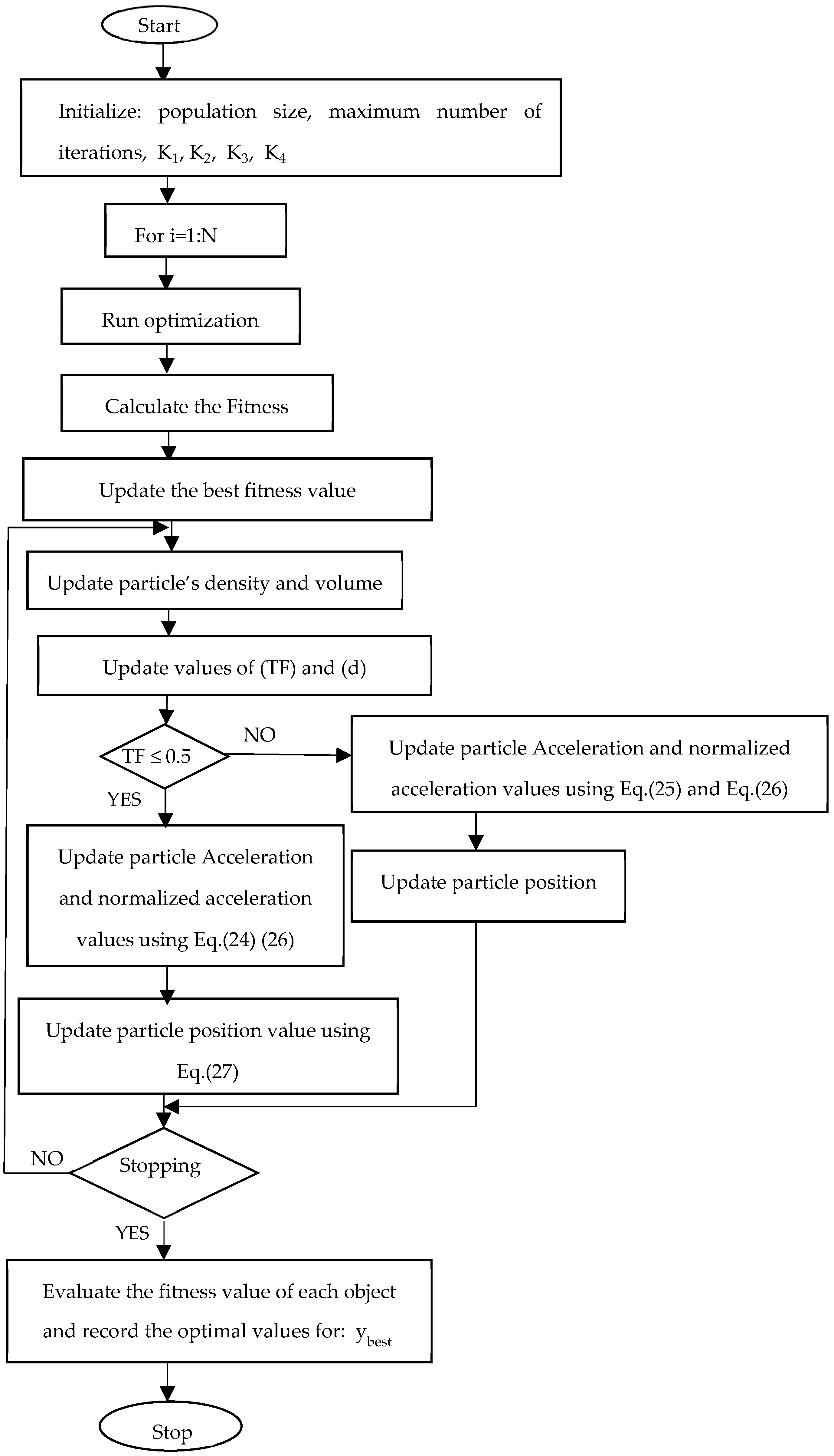
To summarize the preceding equations of the AOA method, Figure 5 depicts the steps needed to execute the algorithm.

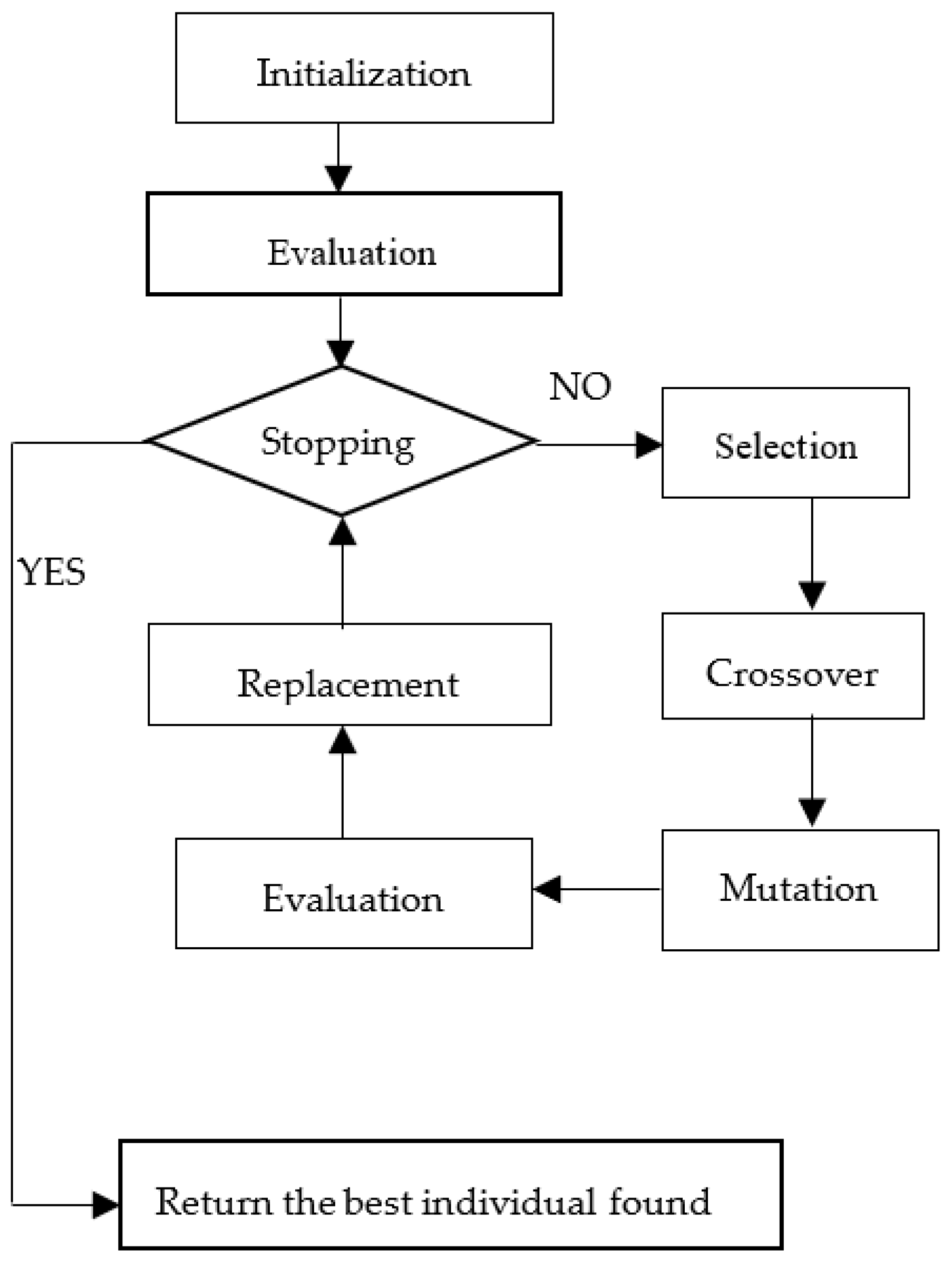
3.2. Overview of the GA and Stages

3.2.1. GA Overview

The GA is a strong search heuristic-based method used to resolve any optimization problems [51]. The GA’s technique is based on the phenomena of natural selection and survival. The law of survival of the strongest allows the GA to discover the best solution after many iterative operations. The GA search technique is based on biology principles, such as natural selection, mutation, and crossover. In general, the GA method begins by producing a random population with numerous chromosomes. Immediately after the population is generated, each member begins to assess a solution, where the solution assessment at each stage is within the purview of either fitness or objective function [52].

The objective of utilizing the GA is to optimally calculate the values of ${\mathrm{K}}_{\mathrm{P}}$ and ${\mathrm{K}}_{\mathrm{i}}$ of the DC-DC chopper. The proportional gain and integral time constant values of the PI controllers in the SMES system are considered as the GA population. The objective is to reach optimized values of the SMES system’s injected active and reactive power to the system.

The GA is utilized to assess the objective function.

3.2.2. GA Stages

• Stage 1: Initialization of the population.
• Stage 2: Fitness function.
• Stage 3: Selection.
• Stage 4: Reproduction.
  Generation of off springs happens in two ways:

  -

  Crossover.

  -

  Mutation.

• Stage 5: Convergence (when to stop).

The pseudo code for the GA algorithm [53] is presented as below (Algorithm 2):

Algorithm 2: Pseudo code of the GA

Initialize random population; Evaluate the population; Generation = 0; while termination criterion is not satisfied do Generation = Generation + 1; Select good chromosome by reproduction procedure; Perform crossover; Perform mutation; Evaluate the population; end while

To summarize the preceding stages of the GA method, Figure 6 depicts the steps needed to execute the algorithm.

3.3. Overview of PSO and Stages

3.3.1. PSO Overview

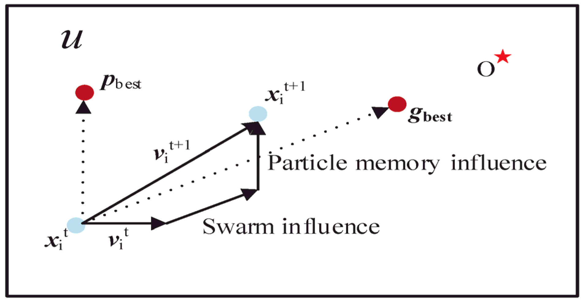
Particle swarm optimization (PSO) is a population-based, stochastic evolutionary computer technique for problem-solving [54]. It is a type of swarm intelligence, based on socio-psychological concepts, that gives insights into social behavior while also contributing to technical applications. James Kennedy and Russell C. Eberhart originally described the particle swarm optimization technique in 1995. A fitness function can be used to evaluate a suggested solution to a given problem. A communication structure or social network is also developed, with neighbors assigned to each participant based on random guesses about issue solutions. They are also referred to as particles; thus, the term particle swarm. An iterative procedure for improving these possible solutions is initiated. The particles evaluate the fitness of the possible solutions repeatedly and remember the position where they had the most success. Individual best solutions are referred to as particle best or local best. Another best value monitored by PSO is the best value acquired so far by any particle in that particle’s neighborhood. This value is entitled ${\mathrm{G}}_{\mathrm{BEST}}$. The primary concept of PSO lies in accelerating each particle to its ${\mathrm{P}}_{\mathrm{BEST}}$ and ${\mathrm{G}}_{\mathrm{BEST}}$ locations, with a random weighted acceleration at each step, as depicted in Figure 7.

The objective of utilizing PSO is to optimally calculate the values of ${\mathrm{K}}_{\mathrm{P}}$ and ${\mathrm{K}}_{\mathrm{i}}$ of the DC-DC chopper. PSO keeps updating the values of the individual and global best fitness values (${\mathrm{P}}_{\mathrm{BEST}}$ and ${\mathrm{G}}_{\mathrm{BEST}}$) of the particles until reaching the minimum value of the fitness function.

The updating procedure of the particle position is shown in the following equations [35,40,54]:

$${\mathrm{V}}_{\mathrm{i}}^{\mathrm{N}+1 }=\mathrm{W}·{\mathrm{V}}_{\mathrm{i}}^{\mathrm{N} }+{\mathrm{C}}_1·{\mathrm{X}}_1 \left({\mathrm{P}}_{\mathrm{BESTi}}^{\mathrm{N} }-{\mathrm{S}}_{\mathrm{i}}^{\mathrm{N}}\right)+{\mathrm{C}}_2·{\mathrm{X}}_2 \left({\mathrm{G} }_{\mathrm{BESTi}}^{\mathrm{N} }-{\mathrm{S}}_{\mathrm{i}}^{\mathrm{N}}\right)$$

(29)

$${\mathrm{S}}_{\mathrm{i}}^{\mathrm{N}+1 }={\mathrm{S}}_{\mathrm{i}}^{\mathrm{N} }+{\mathrm{V}}_{\mathrm{i}}^{\mathrm{N}+1 } \mathrm{i}=1, 2, \dots , \mathrm{M}$$

(30)

where ${\mathrm{V}}_{\mathrm{i}}^{\mathrm{N}+1}$ is the velocity of the particle i in $\mathrm{N}+1$th iteration, W is the inertia weight, ${\mathrm{V}}_{\mathrm{i}}^{\mathrm{N}}$ is the velocity of the particle i in $\mathrm{N}$th iteration, ${\mathrm{C}}_{1 }{\mathrm{and} \mathrm{C}}_2$ are the cognitive parameter and social parameter, respectively, ${\mathrm{X}}_1 \mathrm{and} {\mathrm{X}}_2$ are random numbers, ${\mathrm{P}}_{\mathrm{BESTi}}$ is the best position of $\mathrm{i}$th particle in the swarm, M is the number of particles in the swarm, ${\mathrm{S}}_{\mathrm{i}}^{\mathrm{N}}$ is the $\mathrm{i}$th particle in the swarm in $\mathrm{N}$th iteration, ${\mathrm{G}}_{\mathrm{BESTi}}^{ }$ is the best position of all swarm particles, ${\mathrm{S}}_{\mathrm{i}}^{\mathrm{N}+1}$ is the $\mathrm{i}$th particle in the swarm in $\mathrm{N}+1$th iteration, and N is the number of iteration.

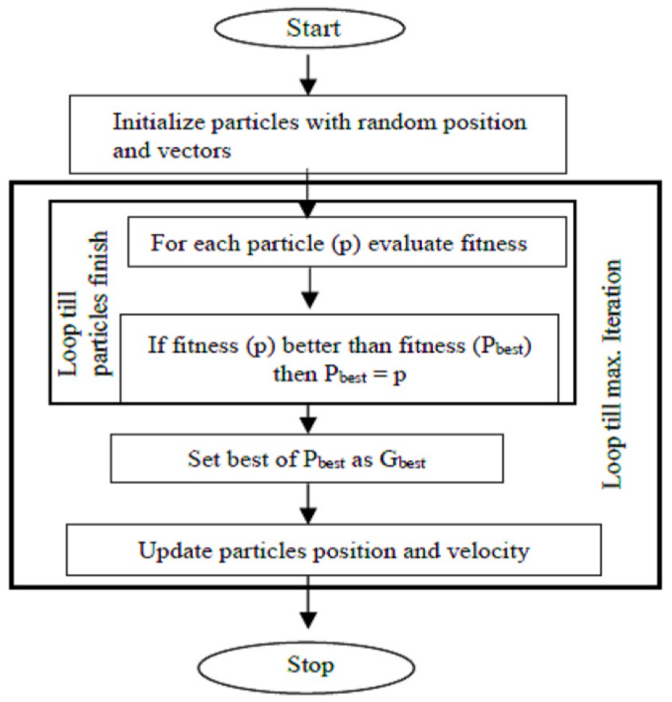
3.3.2. PSO Stages

The PSO technique can be summarized in five steps, which are repeated until the stopping criteria are fulfilled:

• Stage 1: Initialization.
• Stage 2: Fitness evaluation.
• Stage 3: Update the best data.
• Stage 4: Update the velocity and position.
• Stage 5: Convergence determination.

The pseudo code for the PSO algorithm [55] is presented as below (Algorithm 3):

Algorithm 3: Pseudo code of PSO

Begin For each particle in the swarm Initialize its position & velocity randomly end for do for each particle in the swarm Evaluate the fitness function If the objective fitness value is better than the personal best objective fitness value (PBEST) in history, current fitness value set as the new personal best (PBEST) end if end for From all the particles or neighborhood, choose the particle with best fitness value as the (GBEST) for each particle in the swarm Update the particle velocity Update the particle position end for until stopping criteria is satisfied end begin

These steps are illustrated in the flowchart presented in Figure 8.

4. Application of the Optimization Algorithms to the System

The objective or the fitness function is ▲P², which is required to be minimized in order to reduce system error where ▲P = $({\mathrm{P}}_{\mathrm{L} }-{ \mathrm{P}}_{\mathrm{Lref}}$) and the system variables X1 and X2 are the values of ${\mathrm{K}}_{\mathrm{P}}$ and ${\mathrm{K}}_{\mathrm{i}}$ of the DC-DC chopper PI controller. The aim of utilizing different optimization algorithms is to find the optimum values of system variables that correspond the minimum value of the fitness function. The process of selecting the optimum values is bounded by system constraints that are based on the boundaries of the design variables or the model parameters. These constraints are 1 ≤ X1 ≤ 2, 0 ≤ X2 ≤ 1.

The AOA characteristics are presented in

Table 1. AOA characteristics.

AOA Characteristics
Population size	50
${\mathrm{C}}_1$	2
${\mathrm{C}}_2$	6
${\mathrm{C}}_3$	2
${\mathrm{C}}_4$	0.5
Number of iterations	100

.

The GA characteristics are presented in

Table 2. GA characteristics.

GA Characteristics
Population type	Double vector
Population size	50
Selection function	Uniform
Crossover function	Scattered
Mutation function	0.3
Number of iterations	100

.

The PSO characteristics are presented in

Table 3. PSO characteristics.

PSO Characteristics
Number of particles	50
Initial velocity of the particle	0
Inertia weight	1
Acceleration constants	2
Number of iterations	100

.

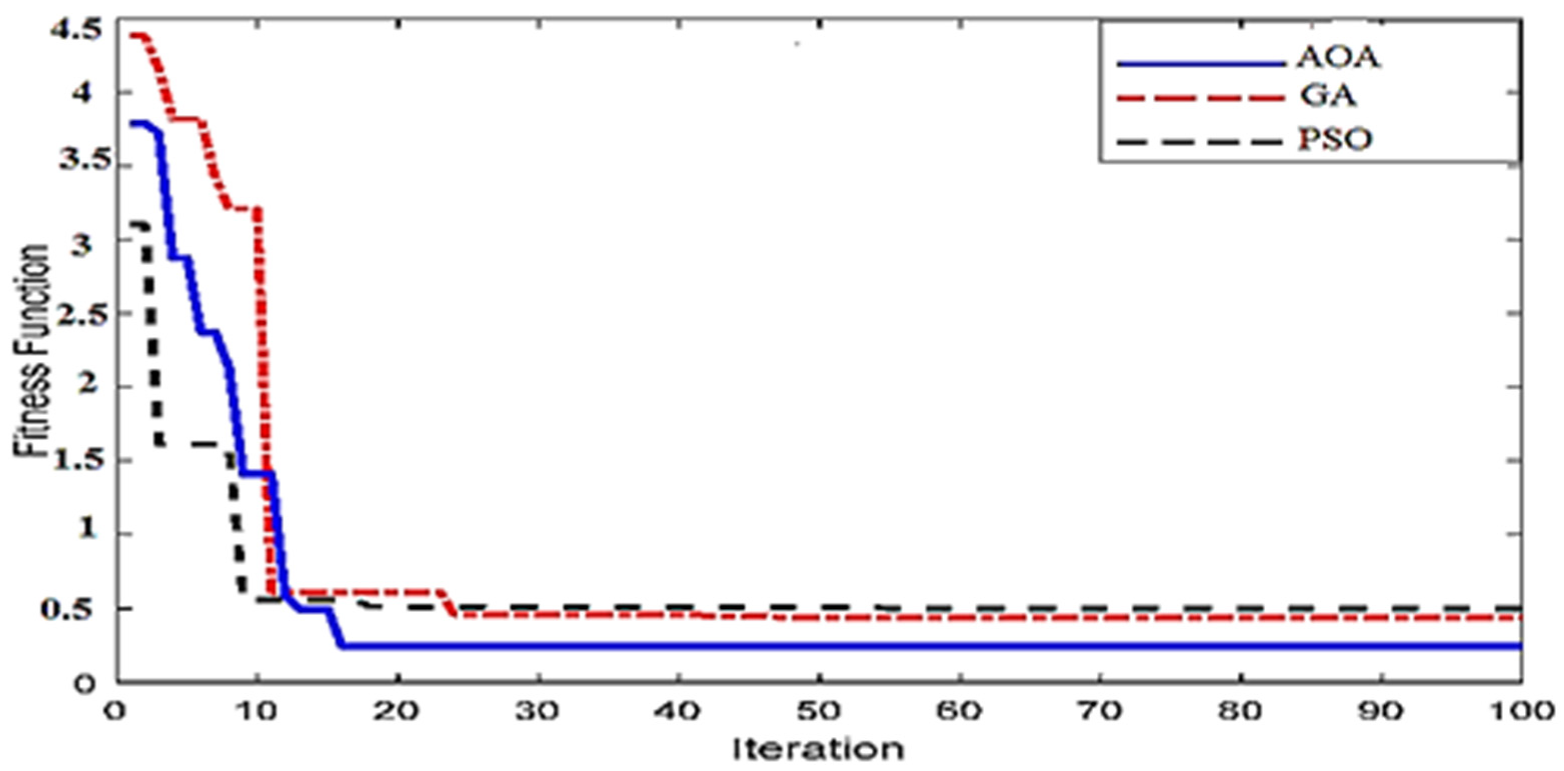
The optimization problem under study was tested under many runs with different operating conditions. These simulations were carried out using the MATLAB program, MATLAB 8.0.604 (2014b) 64-bit version, and executed on the computation environment and the PC comprised of an Intel Core i7 CPU 2.00 GHz, 2.5 GHz, 8 GB RAM, and 64-bit operating system. The wind system model was built using SIMULINK and the proposed optimization techniques’ codes were created using the MATLAB environment. The optimal settings of the optimization algorithms include 50 population agents and 100 iterations. Indeed, these settings were selected to obtain accurate results. To check the robustness of the proposed optimization algorithms, 100 independent simulation runs were performed.

The developed MATLAB codes for all optimization algorithms were customized, based on the above characteristics, to suit the optimization problem. The technology of the MATLAB optimization was utilized to link the optimization codes with the wind SIMULINK model, in order to perform the online optimization process and obtain the results with maximum accuracy.

Several runs were performed, and the best values were chosen. Figure 9 shows the convergence curve of objective function using the AOA, PSO, and GA techniques. Remarkably, the convergence curve is quite smooth, with no oscillations, and it arrives at its final value promptly.

5. Case Study and Simulation Results

This case study shows how the AOA optimization technique may be used to optimize the PI controllers’ parameters that are required to control both the real and reactive powers of the SMES system unit, to improve a grid-connected wind farm’s LVRT capability. The SMES system used a sinusoidal pulse width modulation voltage source converter and a PI-controlled DC-DC converter as its control strategy. The PI control scheme was used to control the VSC. The AOA technique was used to design all PI controllers’ parameters in the SMES system. The effectiveness of the proposed AOA technique for PI-controlled SMES system energy storage was then compared with that of a GA technique and a PSO technique, taking into consideration symmetrical and asymmetrical fault conditions. The MATLAB codes for the three optimization techniques were developed and linked to the Simulink model for the system under study and simulations were conducted using the MATLAB/Simulink program. The simulation outcomes were presented in context, with the latest grid code set by E. 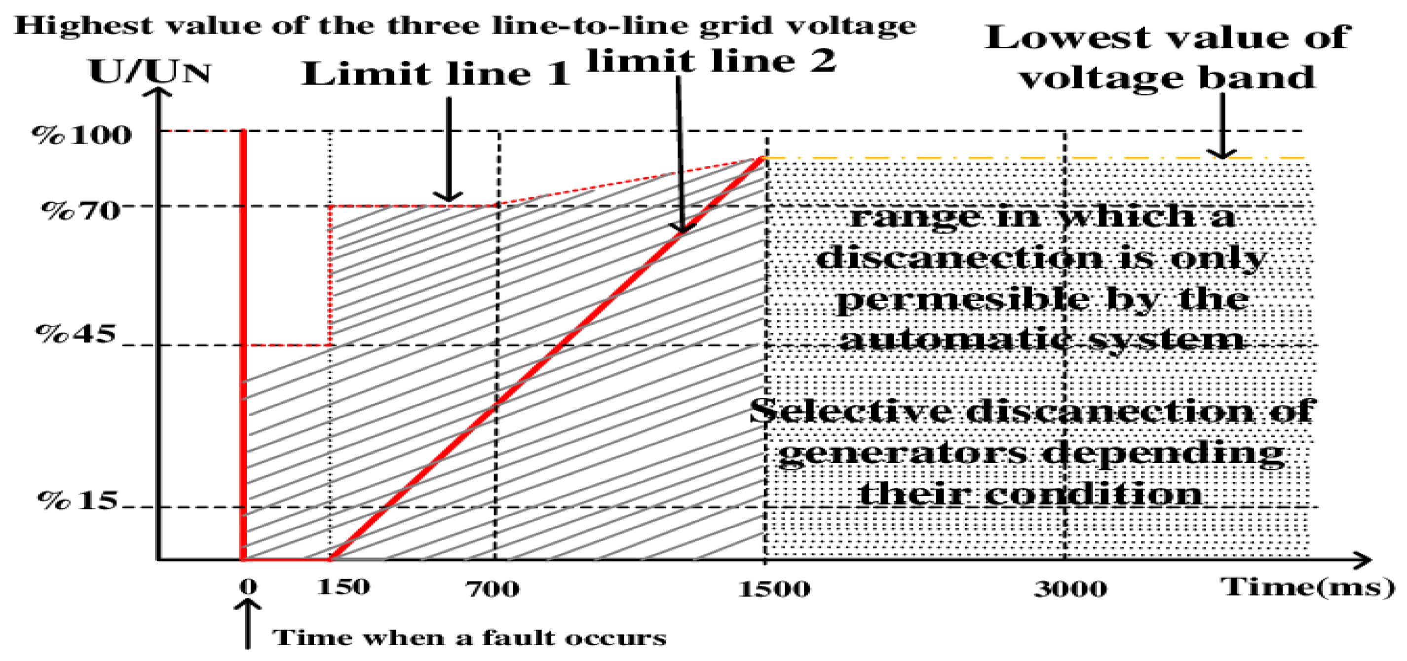On Netz [11]. The LVRT requirement of the grid code is illustrated in Figure 10, where the wind turbines must remain online and linked to the network, above the determined limit lines. The optimization settings included using a population of 50 and 100 iterations; these numbers were chosen in order to reach accurate results.

The different scenarios in this case study are described as follows:

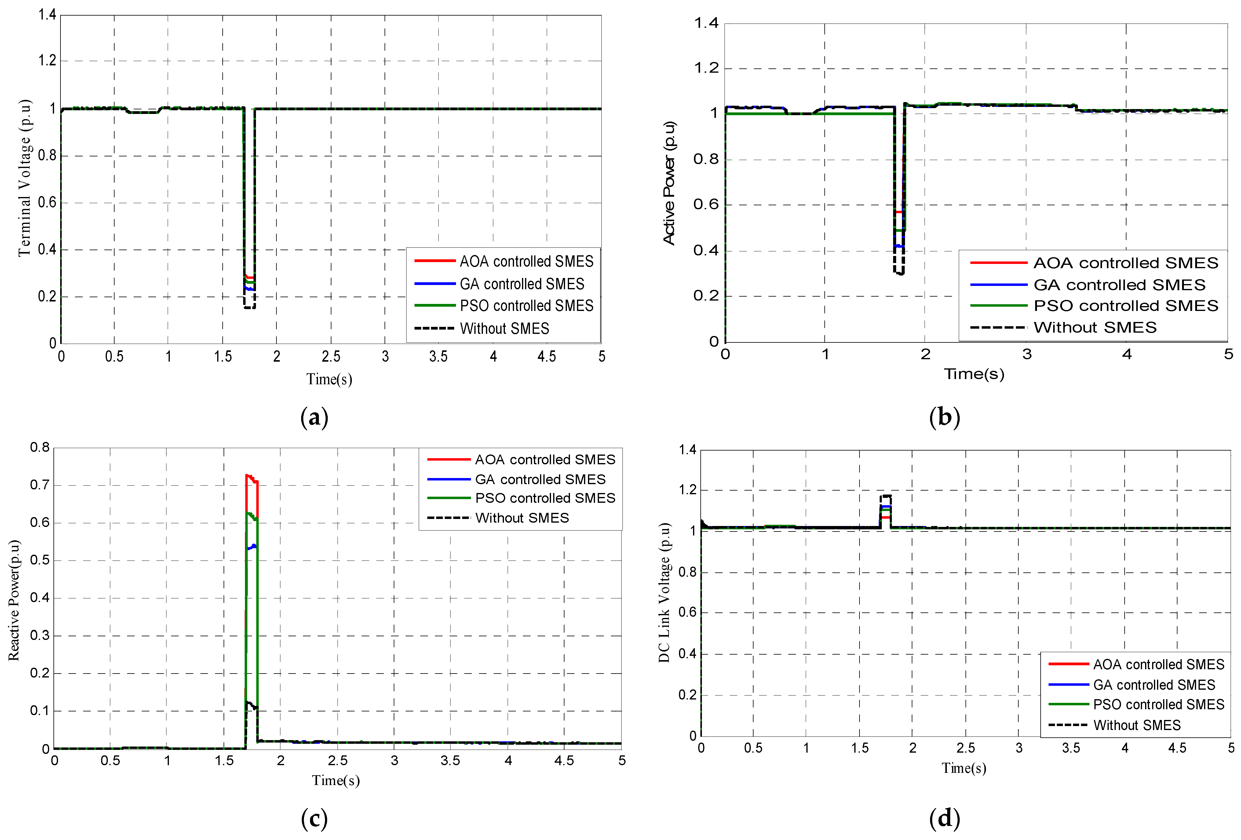
5.1. Three Line-to-Ground (L-L-L-G) Fault Scenario

In this scenario, the system is vulnerable to a significant symmetrical (L-L-L-G) fault. The fault happens at 1.7 s and is located in the system as indicated before in Figure 1.

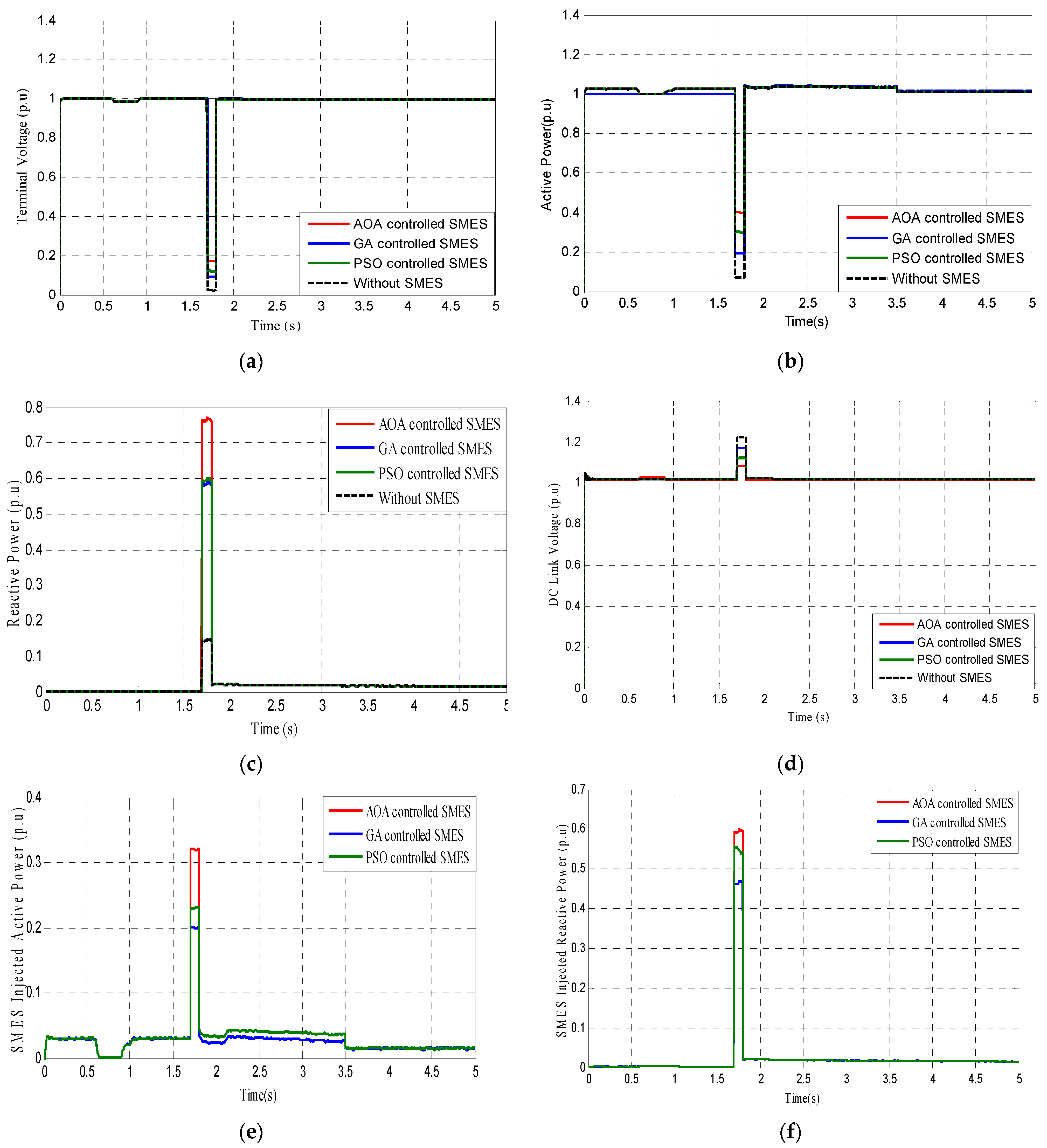
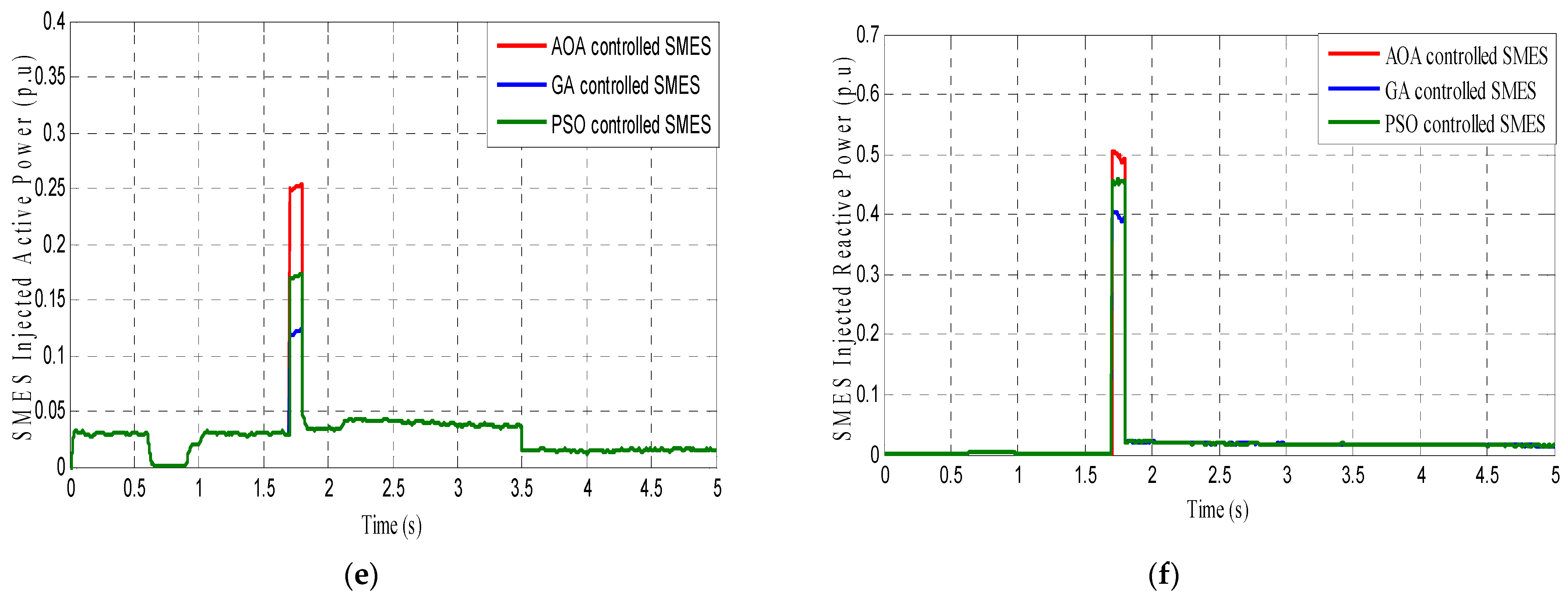
As a subsequent response to the fault, the circuit breakers open at 1.8 s. The circuit breakers effectively terminate the fault at 2.1 s and re-closes safely. Figure 11a illustrates that without utilizing the SMES system, the value of PCC voltage significantly drops. When the SMES system is used, the VSC of the SMES system supplies a sufficient amount of reactive power that overcomes the significant drop in PCC voltage. Moreover, the DC-DC converter of the SMES system supplies and manages the flow of the real power during the abnormal condition. From the simulation results, it was clearly noticeable that when an AOA-optimized SMES unit is utilized, the PCC voltage response is improved, compared to using a GA-optimized SMES unit Figure 11b illustrates the active power (P) response; Figure 11c depicts the reactive power (Q) response, which becomes further improved using the AOA.

Figure 11d illustrates that the DC link voltage has an improved transient characteristic in an AOA-optimized SMES system. It should be highlighted that an AOA-based SMES unit achieves greater responsiveness and efficiency than a PSO-based SMES unit, and a PSO-based SMES unit achieves greater responsiveness and efficiency than a GA-based SMES unit.

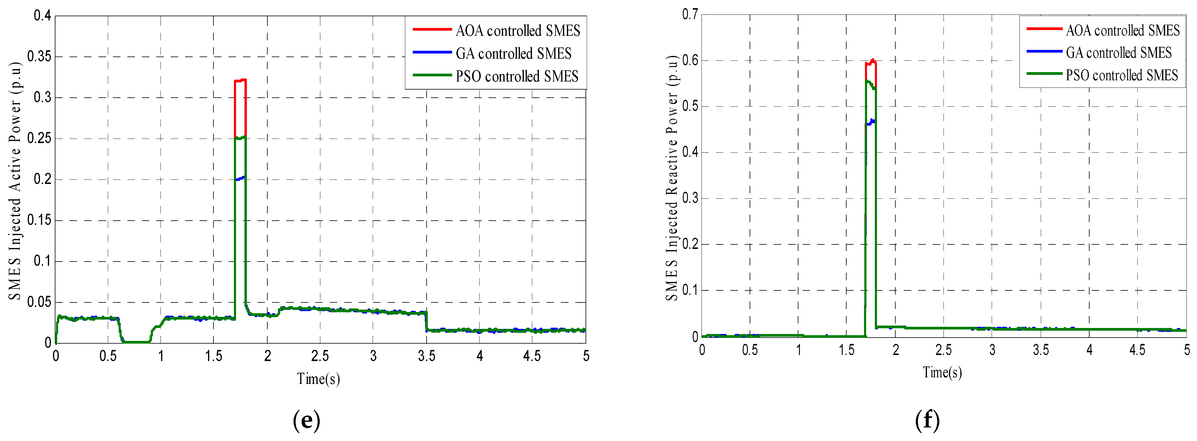
Figure 11e,f illustrates the injected active and reactive power from the SMES unit to the power system.

It can be concluded that when the SMES unit injects more active and reactive power into the system, the system’s performance is enhanced during fault conditions.

A comparison between the optimal PI controller’s value for the AOA, the GA, and PSO is presented in

Table 4. Optimized PI Parameters for L-L-L-G scenario.

	AOA		PSO		GA
PI parameter	${\mathrm{K}}_{\mathrm{p}}$	${\mathrm{K}}_{\mathrm{i}}$	${\mathrm{K}}_{\mathrm{p}}$	${\mathrm{K}}_{\mathrm{i}}$	${\mathrm{K}}_{\mathrm{p}}$	${\mathrm{K}}_{\mathrm{i}}$
value	1.2	0.2	1.15	0.1	1.05	0.08

.

A comparison between SMES-injected active and reactive power values for the AOA, the GA, and PSO is presented in

Table 5. SMES-injected active and reactive power for L-L-L-G scenario.

	AOA		PSO		GA
SMES-injected P and Q values	P	Q	P	Q	P	Q
	0.32	0.6	0.24	0.55	0.2	0.48

.

5.2. Line-to-Line-Toground (L-L-G) Fault Scenario

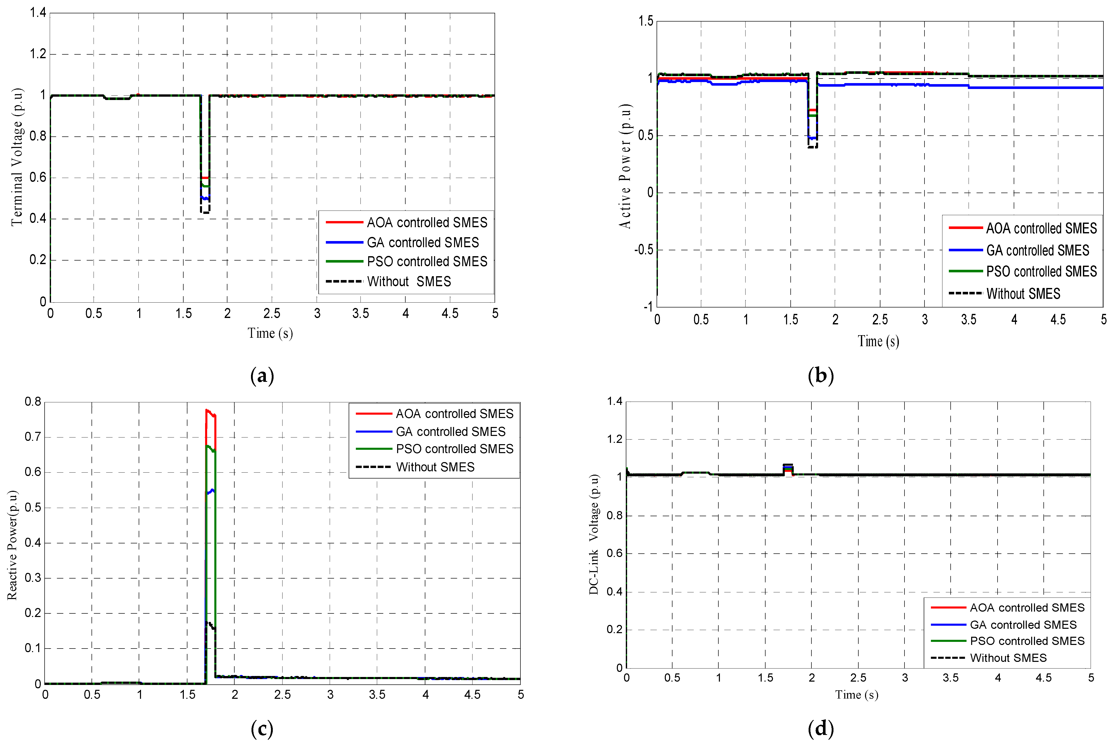
In this scenario, the system is exposed to an asymmetrical L-L-G fault. The system’s different responses are depicted in Figure 12. The response of the terminal voltage has a small error and but fine characteristics. The active power transmitted into the system is greater when utilizing the AOA technique rather than PSO or the GA, which helps in maintaining the system’s stability. The reactive power injected into the system is better in the case of PSO, when compared to the GA. The DC link voltage response is in its best condition in the case of the AOA. It should be highlighted that the AOA tactic is efficient, with asymmetrical faults. Due to the fact that the AOA is a population-based metaheuristic optimization tactic that solves complicated optimization problems in a short duration of time, the response of the system is enhanced when compared to the GA and PSO systems’ responses.

The effectiveness of the proposed AOA technique is also demonstrated in the response of SMES-injected active and reactive power, as in case of the AOA, a larger amount of power is injected into the system during the fault condition to overcome the negative impacts of the fault on the system’s response.

The amount of the injected active and reactive power is determined by the duty cycle of charging and discharging of the SMES coil. The optimal selection of the values of ${\mathrm{K}}_{\mathrm{P}}$ and ${\mathrm{K}}_{\mathrm{i}}$ helps in improving the system’s performance.

A comparison between the optimal PI controller’s values for the AOA, the GA, and PSO is presented in

Table 6. Optimized PI Parameters for L-L-G scenario.

	AOA		PSO		GA
PI parameter	${\mathrm{K}}_{\mathrm{p}}$	${\mathrm{K}}_{\mathrm{i}}$	${\mathrm{K}}_{\mathrm{p}}$	${\mathrm{K}}_{\mathrm{i}}$	${\mathrm{K}}_{\mathrm{p}}$	${\mathrm{K}}_{\mathrm{i}}$
value	1.25	0.28	1.17	0.13	1.09	0.09

.

A comparison between SMES-injected active and reactive power values for the AOA, the GA, and PSO is presented in

Table 7. SMES-injected active and reactive power for L-L-G scenario.

	AOA		PSO		GA
SMES-injected P and Q values	P	Q	P	Q	P	Q
	0.33	0.57	0.25	0.54	0.18	0.44

.

5.3. Line-to-Line (L-L) Fault Scenario

In this scenario, the system is subjected to an L-L fault. As shown in Figure 13, the active and the reactive power performances are improved utilizing the AOA optimization technique. The simulation results show that the responses of the active power and the reactive power are improved when utilizing the AOA-controlled SMES system, compared to not utilizing the SMES system. In the cases of both the terminal and DC link voltages’ responses, the AOA tactic shows that the voltages’ values in the moment that fault occurs do not deviate widely from normal values, which is an indication of stable system response. The positive effect of the SMES system on the system response is clearly demonstrated in the simulation results when compared to the response when not utilizing the SMES system, which is due to its rapid charging and discharging capabilities that enhance the system’s response times.

The amount of injected power from the SMES system reaches its optimum level when utilizing the AOA technique, which positively affects the response of the system.

The simulation graphs show that PSO is not only a strong competitor for the GA technique; it also proved to be more effective than the GA.

A comparison between optimal PI controller’s values for the AOA, the GA, and PSO is presented in

Table 8. Optimized PI parameters for (L-L) scenario.

	AOA		PSO		GA
PI parameter	${\mathrm{K}}_{\mathrm{p}}$	${\mathrm{K}}_{\mathrm{i}}$	${\mathrm{K}}_{\mathrm{p}}$	${\mathrm{K}}_{\mathrm{i}}$	${\mathrm{K}}_{\mathrm{p}}$	${\mathrm{K}}_{\mathrm{i}}$
value	1.28	0.29	1.2	0.17	1.11	0.1

.

A comparison between SMES-injected active and reactive power values for the AOA, the GA, and PSO is presented in

Table 9. SMES-injected active and reactive power for (L-L) scenario.

	AOA		PSO		GA
SMES-injected P and Q values	P	Q	P	Q	P	Q
	0.26	0.59	0.21	0.54	0.15	0.45

.

5.4. Line-to-Ground (L-G) Fault Scenario

In this scenario, the system is subjected to another asymmetrical fault, i.e., the line-to-ground fault (L-G). Figure 14 shows that the system response curves are improved and return quickly to the pre-fault conditions. The positive impact of selecting a strong optimization technique is clearly demonstrated in the response of the system and the active and reactive power injected by the SMES unit. The DC link voltage response shows that there is no sizeable difference between using the GA or PSO techniques, as their results are relatively close to each other. With respect to terminal voltage, PSO shows more effectiveness than the GA. The correct selection of the optimization technique, along with the selection of the correct storing device, has a great measurable impact on the system response, which can be clearly detected in the quick return to the pre-fault state, in addition to the system’s response during the fault, which does not deviate significantly from the normal state. All of these steps lead to a more stable system.

The simulation results show that when the value of the injected SMES system’s active and reactive power increases, the power system shows a more stable response, represented in the decreasing gap between the value of voltage during the fault and the normal operating voltage value.

A comparison between the optimal PI controller’s value for the AOA, the GA, and PSO is presented in

Table 10. Optimized PI parameters for L-G scenario.

	AOA		PSO		GA
PI parameter	${\mathrm{K}}_{\mathrm{p}}$	${\mathrm{K}}_{\mathrm{i}}$	${\mathrm{K}}_{\mathrm{p}}$	${\mathrm{K}}_{\mathrm{i}}$	${\mathrm{K}}_{\mathrm{p}}$	${\mathrm{K}}_{\mathrm{i}}$
value	1.29	0.3	1.25	0.19	1.15	0.18

.

A comparison between the SMES system’s injected active and reactive power values for the AOA, the GA, and PSO is presented in

Table 11. SMES-injected active and reactive power for L-L scenario.

	AOA		PSO		GA
SMES-injected P and Q values	P	Q	P	Q	P	Q
	0.25	0.5	0.17	0.47	0.13	0.4

.

5.5. Normal System Scenario

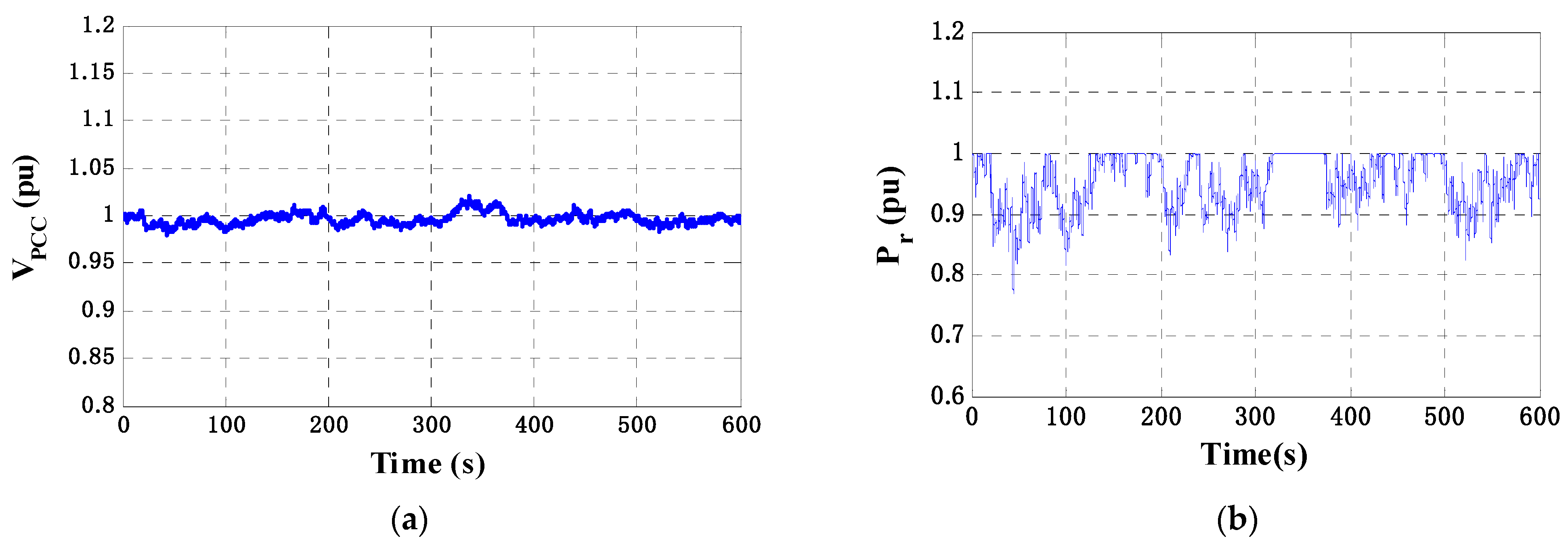
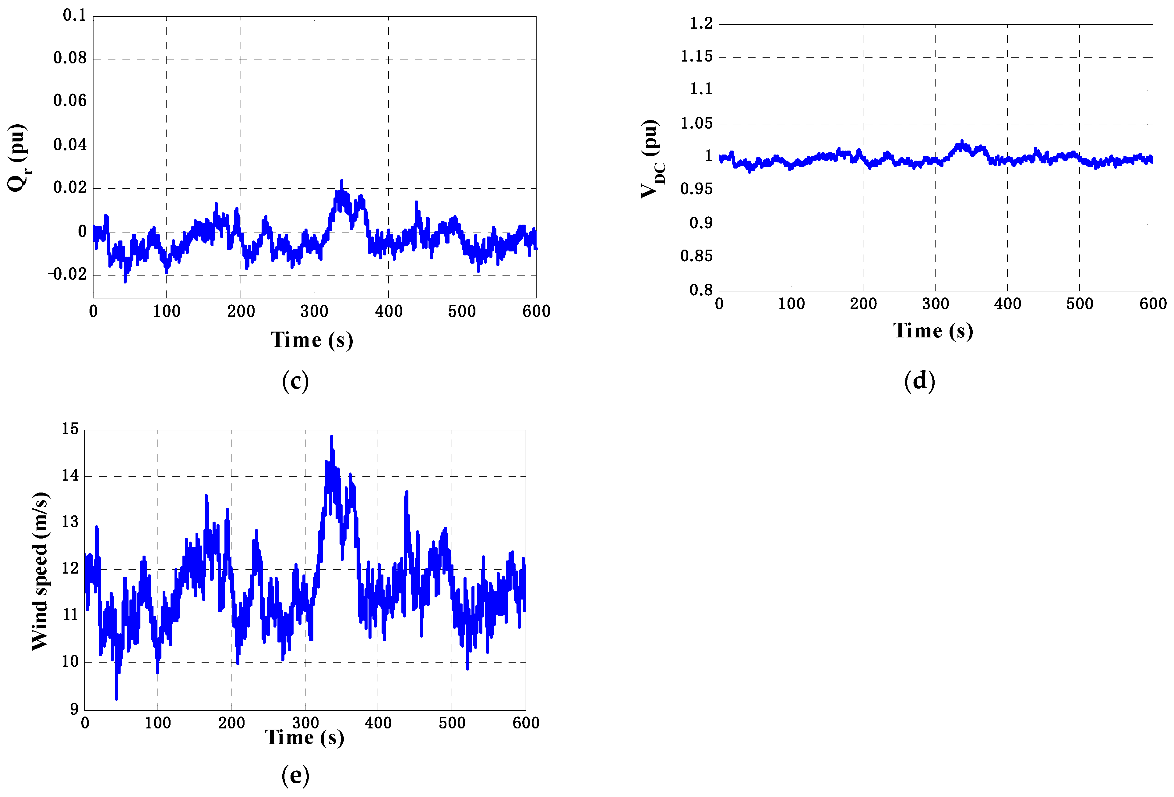
For obtaining authentic system outputs, actual information of wind speed captured from the Zafarana wind farm in Egypt was used, as depicted in Figure 15. The duration of the simulation was 600 s.

From the simulation results, it can be clearly noticed that the actual PCC voltage response has many fluctuations and does not have a smooth response. Figure 15b illustrates the active power (P) response, which is clearly not stable and fluctuates over time, with a negative impact on the system’s response. Figure 15c depicts the reactive power (Q) response, which is also clearly not stable.

Figure 15d illustrates that the DC link voltage value varies with time.

After comparing the results, it can be concluded that the system response is enhanced by using the AOA technique for the capture of maximum power and conveyance to the network.

6. Conclusions

Wind energy has played an important role in developing an ecologically friendly low-carbon economy in recent years. This essential role prompted the quest for various optimization strategies to improve the efficiency of wind system responsiveness.

This article presents revolutionary solutions for improving wind system performance, including an innovative optimization technique known as the AOA that has yet to be documented in the literature for improving the LVRT performance of wind farms. Additionally, this article introduces the novel concept of integrating energy storage devices within a wind system, as is present in the SMES units.

In this article, the SMES units and how to control them are explained by utilizing the AOA for optimally designing the PI controllers in the SMES system, and their effect in boosting the grid-connected wind energy system’s LVRT performance.

The efficacy of the selected optimization approach, AOA, is demonstrated by comparing its response to that of the GA and PSO strategies. Simulations for abnormal operating conditions were carried out to increase confidence in the selected optimization technique. The simulation findings demonstrated that an AOA-based SMES unit has a sizeable impact in restoring the system to its normal state before a fault, while also improving the wind system’s LVRT capabilities. Based on the simulation findings, it is apparent that the AOA-based PI controller approach is an excellent strategy, which control designers can apply to improve the behavior of VSWTs and PMSGs.

Further research was conducted by evaluating the result of other published comparative studies in the same field to ensure the efficacy of the recommended solutions [56,57].

More attention should be drawn to studying and analyzing different forms of faults that can affect wind systems and finding appropriate solutions, in order to overcome the negative impacts of these faults on system performance [58,59].

Future work should investigate further improvements to the wind energy conversion systems’ behavior, by combining various optimization approaches with different storing devices. It is expected that the introduced AOA optimization technique will attract many researchers who are interested in the optimization of various power engineering problems, to be tested and applied on different wind systems.

Future research should also be subjected to the enhancement of the optimization techniques, as they are considered to be the core tool for enhancing the stabilization of a wind generator system. Future research directions for the proposed AOA include applications to address new real-world difficulties. This will help to ensure that the strategy is sufficiently adaptive to generate optimum answers to a diverse set of optimization problems.

More future attention should be directed to the energy storage devices presented, in introducing and studying the insertion of more than one type of energy storage device to a wind system, as they showed great importance in improving wind system performance.