Article

A New Family of Continuous Distributions: Properties and Estimation

by
Mohamed Hussein
1,2,*,
Howaida Elsayed
2 and
Gauss M. Cordeiro
3
1
Department of Mathematics and Computer Science, Alexandria University, Alexandria 21544, Egypt
2
Department of Business Administration, College of Business, King Khalid University, Abha 61421, Saudi Arabia
3
Departamento de Estatística, Universidade Federal de Pernambuco, Cidade Universitária, Recife 52070-040, Brazil
*
Author to whom correspondence should be addressed.
Symmetry 2022, 14(2), 276; https://doi.org/10.3390/sym14020276
Submission received: 8 December 2021 / Revised: 18 January 2022 / Accepted: 26 January 2022 / Published: 29 January 2022

Abstract

:
We introduce a new flexible modified alpha power (MAP) family of distributions by adding two parameters to a baseline model. Some of its mathematical properties are addressed. We show empirically that the new family is a good competitor to the Beta-F and Kumaraswamy-F classes, which have been widely applied in several areas. A new extension of the exponential distribution, called the modified alpha power exponential (MAPE) distribution, is defined by applying the MAP transformation to the exponential distribution. Some properties and maximum likelihood estimates are provided for this distribution. We analyze three real datasets to compare the flexibility of the MAPE distribution to the exponential, Weibull, Marshall–Olkin exponential and alpha power exponential distributions.

1. Introduction

The characteristics of classical distributions are limited and cannot represent all situations found in applications or may not provide a good fit in many practical situations. Adding parameters to a parent distribution is an effective way to make it more flexible and to improve the goodness of fit to real data. However, the properties of the generating distribution will need further investigation, as they are, generally, different from those of the parent distribution. There are different methods to include parameters to a distribution. Ref. [1] seems to have been the first to raise an exponential cumulative distribution function (cdf) to a positive power. Exponentiated distributions are also known as proportional reversed hazard rate models with a constant of proportionality α [2] or Lehman alternatives [3]. Ref. [4] added a shape parameter to the normal distribution to obtain a skew-normal distribution. Ref. [5] included an extra parameter α via the transformation G x = F ( x ) / [ 1 ( 1 α ) F ¯ x ] , which transforms any cdf F ( · ) to a new cdf G ( · ) , where F ¯ x = 1 F x . Ref. [6] added two parameters ( r , p ) to the survival function by considering a countable mixture of positive integer powers of general survival functions, where the mixing proportions are Pascal (r,p). Ref. [7] included two parameters to any probability density function (pdf), based on the form of a mixture, to construct a new family. Ref. [8] defined a method of adding a parameter to a parent distribution called the alpha power (AP) transformation. Henceforth, the pdf and cdf of any continuous baseline random variable W are denoted by f ( · ) and F ( · ) , respectively. Then, the cdf of the AP family (for x R ) has the form
F AP ( x ) = α F ( x ) 1 α 1 , if α > 0 , α 1 ,
and the corresponding pdf has the form
f AP ( x ) = log α α 1 α F ( x ) f ( x ) .
The AP transformation has been used by many authors to construct new distributions from baseline models. Among others, Refs. [8,9,10,11,12,13,14] derived the alpha power exponential (APE), AP Weibull, AP inverse Weibull, AP Lindley, AP Pareto, AP Kumaraswamy and AP Gompertz distributions from the exponential, Weibull, inverse Weibull, Lindley, Pareto, Kumaraswamy and Gompertz distributions, respectively. Ref. [15] introduced the three-parameter AP transformed extended exponential, which includes the AP transformed exponential and AP transformed Lindley distributions. Ref. [16] defined the cdf of an extended AP class (say “EAP”) (for x R )
F EAP x = α F ( x ) e F ( x ) α e , if α > 0 , α e .
Recently, Ref. [17] included a new parameter by combining the type II half-logistic-G family with the inverted Topp–Leone distribution to define the half-logistic inverted Topp–Leone family. In this paper, we propose a modified alpha power (MAP) family by adding two parameters to a baseline model. Therefore, the properties of the generated distributions require further investigation, as they are different from those of the baseline models. We apply the new transformation to the exponential distribution to construct the modified alpha power exponential (MAPE) distribution.
The paper is organized as follows: Section 2.1 defines the MAP family and provides a linear representation for its density function to derive some of its properties. Section 2.2 determines the MAPE distribution, addresses some of its properties and estimates the unknown parameters. A statistical analysis of two real datasets to verify the effectiveness of the proposed model is reported in Section 3. Some conclusions are offered in Section 4.

2. Materials and Methods

2.1. The MAP Transformation

Definition 1.
For every continuous cdf F ( x ) , the cdf of the new MAP family is defined by the monotonic increasing cdf G : R [ 0 , 1 ] (for x R )
G x = β F 2 x α F x 1 α β 1 , if α , β 1 , α β 1 .
The main motivation for (1) follows from the fact that the new family succeeds in fitting real data as a competitive model to widely applied classes. Clearly, we can adopt β F γ ( x ) for an unknown parameter γ > 0 , but this will lead to a model with three extra parameters. This proposal can be investigated following the same lines of the MAP family.
It is clear that
  • lim x G x = 0 and lim x G x = 1 .
  • For β = 1 and α 1 , G ( x ) F ( x ) , which means that the baseline distribution is a sub-model of the new family.
  • G ( · ) is not defined for α β = 1 ( α = β = 1 ) .
The pdf corresponding to (1) can be expressed as
g x = 1 α β 1 β F 2 x α F x ln α + 2 F x ln β f x .
Equation (2) is a weighted version of the baseline density f x , where the weight function has the form
w x = β F 2 x α F x ln α + 2 F x ln β .
Thus,
E w X = β F 2 x α F x ln α + 2 F x ln β f x d x = α β 1 .
Therefore, Equation (2) can be expressed as
g x = 1 α β 1 w x f x .
Such weighted distributions play an important role in distribution theory [18].
Figure 1 and Figure 2 show the effects of the extra parameters on the cdf and pdf of some parent distributions. Clearly, we can control the skewness and kurtosis of the generated distributions through the extra parameters. For an exponential distribution with decreasing pdf, the new transformed exponential pdf is a concave function. The plots in Figure 2 reveal that the parameters α and β can produce asymmetrical densities to the right and left and change tail lengths.

2.1.1. Linear Representation

The two power series hold
β F 2 x = e F 2 x ln β = i = 0 ln β i i ! F x 2 i ,
and
α F x = e F x ln α = j = 0 ln α j j ! F x j .
Therefore, the cdf of the MAP distribution (1) can be expressed as
G x = 1 α β 1 i , j = 0 ψ i , j α , β F x 2 i + j 1 ,
where ψ i , j α , β = ln α j ln β i / ( i ! j ! ) (for i , j 0 ).
Then, the MAP family density (2) can be expressed as
g x = 1 α β 1 i , j = 0 ; 2 i + j 1 2 i + j ψ i , j α , β F x 2 i + j 1 f ( x ) ,
and then
g x = 1 α β 1 i , j = 0 ; 2 i + j 1 ψ i , j α , β π 2 i + j ( x ) ,
where π 2 i + j ( x ) = 2 i + j F x 2 i + j 1 f ( x ) is the exponentiated-F (exp-F) density with power parameter 2 i + j (for 2 i + j 1 ).
Hence, based on the linear representation (5), we can obtain directly some mathematical properties (ordinary and incomplete moments, generating function and mean deviations, among others) of the MAP family from those properties of the exp-F distributions, which were reported in several papers; see Table 1 of [19]. Some other properties, such as different types of entropy, reliability and order statistics, and their computations may be addressed in future research.
For a specific F ( x ) , these properties can also be calculated approximately from (4) by well-known methods of numerical integration; see, for example, [20].

2.1.2. Mode

The mode x * of the MAP family can be found by maximizing the log-pdf from (2)
ln g ( x ) = ln α β 1 + F 2 x ln β + F x ln α + ln f x + ln ln α + 2 F x ln β .
At x = x * , the derivative of ln g ( x ) with respect to x vanishes. We can obtain the mode of the MAP family by solving the following equation
2 F x * f x * ln β + f x * ln α + f x * f x * + 2 f x * ln β ln α + 2 F x * ln β = 0 ,
which has no explicit solution for x * . Therefore, the mode of the MAP family does not have a closed form. Given F ( · ) and f ( · ) , direct maximization of ln g ( x ) using a numerical optimization algorithm or a one-dimensional root-finding algorithm of (6) can give an approximation for the mode.
For simplicity, let a = ln α 0 and b = ln β 0 , since α 1 and β 1 . The first derivative of the log-density is
( ln g ) ( x ) = 2 b f ( x ) F ( x ) + a f ( x ) + ( ln f ( x ) ) + [ ln ( a + 2 b F ( x ) ) ] .
Let K ( x ) = f ( x ) [ a + 2 b F ( x ) ] . Then,
( ln g ) ( x ) = f ( x ) ( 2 b F ( x ) + a ) + ( ln f ( x ) + ln ( a + 2 b F ( x ) ) ) = f ( x ) ( 2 b F ( x ) + a ) + ( ln [ f ( x ) ( a + 2 b F ( x ) ) ] ) = K ( x ) + ( ln K ( x ) ) .
Let J ( x ) = ln K ( x ) . Then, ( ln g ) ( x ) = K ( x ) + J ( x ) and ( ln g ) ( x ) = K ( x ) + J ( x ) .
Hence, a sufficient condition for the unimodality of the MAP density is K ( x ) + J ( x ) 0 , which gives
K ( x ) [ K ( x ) 2 K ( x ) ] + K ( x ) K ( x ) 0 .

2.1.3. Quantiles

There is no explicit form for the quantile function of the MAP distribution, and its qth quantile ( x q ) can be approximated using a one-dimensional root-finding algorithm in G ( x q ) = q .

2.1.4. Survival and Hazard Functions

Let X be a random variable with the MAP family, pdf g ( · ) and cdf G ( · ) . Then, the survival function of X, say S G x = P ( X > x ) , is
S G x = α β α β 1 1 β F 2 x 1 α F x 1 = α β α β 1 1 β S F ( x ) ( S F x 2 ) α S F x .
The hazard rate function (hrf) h G x and the proportional hrf of X are
h G x = β F 2 x 1 α F x 1 ln α + 2 F x ln β f x 1 β F 2 x 1 α F x 1 ,
h G * x = β F 2 x α F x ln α + 2 F x ln β f x β F 2 x α F x 1 .
The cdf of the MAP family (and also for any cdf) can be expressed in terms of the hrf and proportional hrf from [21] as
G x = h G x h G x + h G * x .
Equation (7) can be rewritten as
h G x = β F 2 x 1 α F x 1 ln α + 2 F x ln β 1 F x 1 β F 2 x 1 α F x 1 h F x ,
where h F x = f ( x ) / [ 1 F ( x ) ] is the baseline hrf. Hence, the hrf of the MAP class satisfies the following properties:
lim x h G x = ln α α β 1 lim x h F x ,
and
lim x h G x = lim x h F x .
Figure 3 illustrates, for some parameter values, the effects of the additional parameters on the hrf for some parent distributions (solid line). For example, the exponential distribution has a constant hrf, whereas the MAPE distribution has an increasing hrf.

2.1.5. Random Number Generator

There is no explicit form for the quantile function of the MAP family, say G 1 ( · ) . We can use acceptance–rejection criteria [22] to generate a random variate from the MAP class. Since, for  α , β 1 , α β 1 , we have
g x f x α β ln α + 2 ln β α β 1 ,
and then the acceptance–rejection algorithm can be used as follows:
Step 1: Generate a random variable W from the baseline distribution F.
Step 2: Generate a uniform (0, 1) random variable U (independent of W).
Step 3: If
U g W c f W ,
where c = α β ln α + 2 ln β / ( α β 1 ) , then set X = W (accept); otherwise, go back to step 1 (reject).

2.1.6. Estimation

Let X 1 , , X n be a random sample of size n from the MAP model with parameters ( α , β , θ ), and observed values x 1 , , x n , where θ is the parameter vector of the parent distribution. The log-likelihood function for the full vector of parameters of X has the form
α , β , θ = n ln α β 1 + ln β i = 1 n F 2 x i ; θ + ln α i = 1 n F x i ; θ + i = 1 n ln f x i ; θ + i = 1 n ln ln α + 2 F x i ; θ ln β .
By differentiating α , β , θ with respect to the parameters, we obtain the score components:
U α = n β α β 1 + 1 α i = 1 n F x i ; θ + 1 α i = 1 n 1 ln α + 2 F x i ; θ ln β ,
U β = n α α β 1 + 1 β i = 1 n F 2 x i ; θ + 2 β i = 1 n F x i ; θ ln α + 2 F x i ; θ ln β ,
and
U θ = 2 ln β i = 1 n F x i ; θ + 1 ln α + 2 F x i ; θ ln β F x i ; θ θ + ln α i = 1 n F x i ; θ θ + i = 1 n 1 f x i ; θ f x i ; θ θ .
The maximum-likelihood estimates (MLEs) ( α ^ , β ^ , θ ^ ) are calculated by solving the nonlinear equations U α = 0 , U β = 0 and U θ = 0 . These equations cannot be solved analytically, but we can use iterative techniques such as a Newton–Raphson type algorithm to calculate these estimates. The Broyden–Fletcher–Goldfarb–Shanno method with analytical derivatives can be used for maximizing α , β , θ . Some optimization algorithms for maximizing log-likelihood functions based on swarm intelligence have been proposed over the last decades. One very popular swarm intelligence method is the Particle Swarm Optimization (PSO) [23].

2.2. The MAPE Distribution

Exponential distributions have an important role in the analysis of product reliability and lifetime data. In this section, we define the MAPE distribution by applying the MAP transformation to the exponential distribution with rate parameter λ .
Definition 2.
The random variable X is said to have a three-parameter MAPE distribution, say MAPE α , β , λ , if its cdf is given by
G E x = β 1 e λ x 2 α 1 e λ x 1 α β 1 , if α , β 1 , α β 1 , x > 0 .
The pdf of X (under the same conditions on the parameters) reduces to
g E x = λ α β 1 β 1 e λ x 2 α 1 e λ x e λ x ln α + 2 1 e λ x ln β .
Further, the survival function and hrf of X are
S E x = α β α β 1 1 β e λ x ( e λ x 2 ) α e λ x
and
h E x = λ e λ x β e λ x ( e λ x 2 ) α e λ x ln α + 2 1 e λ x ln β 1 β e λ x ( e λ x 2 ) α e λ x ,
respectively.

2.2.1. Moments

For a random variable X following a MAPE distribution with parameters θ = ( α , β , λ ) , the rth ordinary moment of X (for r = 1 , 2 , ) can be determined from (4) and the well-known moments of the exp-exponential model.
Alternatively, the moments can be expressed as
μ r = 1 λ r α β 1 0 1 β y 2 α y ln α + 2 y ln β ln 1 1 y r d y .
By expanding β y 2 and α y in power series, we can write
μ r = 1 λ r α β 1 i , j = 0 2 i + j ψ i , j α , β 0 1 ln 1 1 y r y 2 i + j d y ,
where ψ i , j was defined in Section 2.1.1.
Alternatively, the rth ordinary moment of X can be expressed as
μ r = r ! α β λ r ( α β 1 ) ln α i , j , k = 0 ψ i , j , k η i , j , k + 2 ln β i , j , k = 0 ψ i , j , k η i , j , k η i , j , k + 1 ,
where
ψ i , j , k = 2 j ln β i + j ln α k / i ! j ! k !
and
η i , j , k = 1 2 i + j + k + 1 r + 1 .
For more details, see the Appendix A.
Table 1 reports the approximate values of some statistics for the MAPE distribution. The mode of X was approximated via direct maximization of ln g E ( x ) using the R optim function and the unit root-finding function for the function
g E x g E x = λ + 2 λ e λ x 1 e λ x + λ e λ x ln α + 2 λ e λ x ln β ln α + 2 1 e λ x ln β .
The quartiles were found using the unit root-finding function for G E x q = 0 ( q = 0.25 , 0.5 , 0.75 ) . These functions are available in Ref. [24].

2.2.2. Estimation

Let X 1 , , X n be a random sample of size n from the MAPE distribution with parameters ( α , β , λ ) and observed values x 1 , , x n . The log-likelihood function for the parameters can be expressed as
α , β , λ = n ln α + ln λ n ln α β 1 + ln β i = 1 n 1 e λ x i 2 ln α i = 1 n e λ x i λ i = 1 n x i + i = 1 n ln ln α + 2 1 e λ x i ln β .
The maximum likelihood equations are
n α n β α β 1 1 α i = 1 n e λ x i + 1 α i = 1 n 1 ln α + 2 1 e λ x i ln β = 0 ,
n α α β 1 + 1 β i = 1 n 1 e λ x i 2 + 2 β i = 1 n 1 e λ x i ln α + 2 1 e λ x i ln β = 0 ,
n λ + 2 ln β i = 1 n x i e λ x i 1 e λ x i + ln α i = 1 n x i e λ x i i = 1 n x i + 2 ln β i = 1 n x i e λ x i ln α + 2 1 e λ x i ln β = 0 .
Like most of the extensions of the exponential distribution, the MLEs of these parameters cannot be obtained in closed form. Therefore, the maximum likelihood equations should be solved numerically. Alternatively, a numerical maximization of the log-likelihood function is a good technique for calculating the estimates of the unknown parameters.
Using large sample approximation, n α ^ , β ^ , λ ^ are asymptotically normally distributed with mean vector 0 and covariance matrix estimated by the inverse of the observed information matrix
I 1 α ^ , β ^ , λ ^ = 2 α 2 2 α β 2 α λ 2 β α 2 β 2 2 β λ 2 λ α 2 λ β 2 λ 2 α = α ^ , β = β ^ , λ = λ ^ 1 ,
where
2 α 2 = n α 2 + n β 2 α β 1 2 + 1 α 2 i = 1 n e λ x i 1 α 2 i = 1 n 1 ln α + 2 1 e λ x i ln β 2 1 α 2 i = 1 n 1 ln α + 2 1 e λ x i ln β , 2 α β = n α β 1 2 2 α β i = 1 n 1 e λ x i ln α + 2 1 e λ x i ln β 2 , 2 α λ = 1 α i = 1 n x i e λ x i 2 ln β α i = 1 n x i e λ x i ln α + 2 1 e λ x i ln β 2 , 2 β 2 = n α 2 α β 1 2 1 β 2 i n 1 e λ x i 2 4 β 2 i = 1 n 1 e λ x i 2 ln α + 2 1 e λ x i ln β 2 2 β 2 i = 1 n 1 e λ x i ln α + 2 1 e λ x i ln β , 2 β λ = 2 β i = 1 n x i e λ x i 1 e λ x i 4 ln β β i = 1 n x i e λ x i 1 e λ x i ln α + 2 1 e λ x i ln β 2 + 2 β i = 1 n x i e λ x i ln α + 2 1 e λ x i ln β , 2 λ 2 = n λ 2 + 2 ln β i = 1 n x i 2 e 2 λ x i ln α i = 1 n x i 2 e λ x i 2 ln β i = 1 n x i 2 e λ x i 1 e λ x i 4 ln β 2 i = 1 n x i 2 e 2 λ x i ln α + 2 1 e λ x i ln β 2 2 ln β i = 1 n x i 2 e λ x i ln α + 2 1 e λ x i ln β .
Thus, the  100 ( 1 τ ) % approximate confidence intervals for α , β and λ can be constructed from the estimated diagonal elements of the above matrix.

2.3. MAP-Normal (MAPN) Model

Henceforth, we work with a random variable Z having the standard MAPN ( α , β , 0 , 1 ) distribution because of the transformation X = μ + σ Z . Then, the density of Z reduces to ( α , β 1 , α β 1 )
G z = β Φ 2 z α Φ z 1 α β 1 ,
where Φ ( z ) is the standard normal cdf.
Some properties of Z can be determined from (5) as
g z = 1 α β 1 i , j = 0 ; 2 i + j 1 2 i + j ψ i , j α , β Φ z 2 i + j 1 ϕ ( z ) ,
where ϕ ( z ) is the standard normal density.
Setting u = Φ ( z ) , we can write μ r = E ( Z r ) in terms of the standard normal qf Q S N ( u ) = Φ 1 ( u ) :
μ r = 1 α β 1 i , j = 0 ; 2 i + j 1 2 i + j ψ i , j α , β 0 1 Q S N ( u ) r u 2 i + j 1 d u .
A power series for the standard normal qf holds [25]
Q S N ( u ) = k = 0 b k 2 π ( u 1 / 2 ) 2 k + 1 ,
where the coefficient b k is calculated recursively from
b k + 1 = 1 2 ( 2 k + 3 ) r = 0 k ( 2 r + 1 ) ( 2 k 2 r + 1 ) b r b k r ( r + 1 ) ( 2 r + 1 ) .
Here, b 0 = 1 , b 1 = 1 / 6 , b 2 = 7 / 120 , b 3 = 127 / 7560 , Therefore, we can evaluate numerically the integral
I r , i , j = 0 1 k = 0 b k 2 π ( u 1 / 2 ) 2 k + 1 r u 2 i + j 1 d u ,
and determine the ordinary moments of the MAPN distribution.
The skewness and kurtosis measures of Z can be calculated from the ordinary moments using well-known relationships. The rth incomplete moment of Z also follows from an integral, as above, by changing one for a convenient constant. The first incomplete moment immediately gives the mean deviations of Z about the mean or any other location.

3. Results

3.1. Simulation Study

A simulation is performed to study the behavior of the MLEs of the parameters α , β and λ of the MAPE distribution in terms of their averages, absolute biases (ABs) and mean square errors (MSEs) of the estimates obtained from 1000 samples under different scenarios for sample sizes n = 50 , 100 , 150 , 200 , 250 . The results are in Table 2.
We compare the MAPE distribution with some other extensions of the exponential distribution, specifically the Beta exponential (Beta-E), Kumaraswamy exponential (Kw-E) and Marshall–Olkin exponential (MOE), using a random sample of size 100 generated from the MAPE distribution with α = 2 , β = 2 and  λ = 0.5 . The sample values are:
1.885041737, 4.986048585, 3.066673918, 0.959772040, 2.825368368, 0.824435649, 1.294124159, 1.012800439, 5.167502802, 1.068702611, 9.623282708, 2.156111659, 5.752932638, 3.670298312, 1.832103403, 8.127591949, 3.185589749, 0.068173249, 3.384436805, 1.746315020, 2.993498932, 12.453617304, 4.934371758, 7.789793514, 2.734155022, 2.642853318, 3.251226831, 7.176859866, 0.203007024, 5.584507972, 1.169154800, 0.437596269, 2.547156770, 1.606106547, 4.204954374, 4.496538512, 1.295321912, 3.177033049, 1.044723861, 1.646249159, 0.645593200, 2.402715247, 6.392833545, 7.284959565, 0.001960174, 4.312072308, 2.283924227, 0.462808553, 6.438231855, 4.652210157, 0.370191192, 3.436350472, 2.670331310, 3.058598962, 0.850709308, 6.201166734, 4.893258106, 3.137402020, 5.488975387, 6.466631233, 4.510068949, 2.098932480, 1.210160010, 0.350602649, 6.132940426, 1.215480205, 3.524247143, 1.599821076, 2.080543331, 1.868623797, 7.776530949, 1.203310307, 6.869488403, 5.233742062, 0.889446491, 4.337990211, 8.693465053, 1.555651987, 0.927514150, 4.653270469, 2.223475490, 2.077584863, 5.174423467, 10.262362345, 3.124613475, 3.487773970, 3.801199648, 2.102226125, 3.247546812, 2.429156739, 4.481736907, 1.595783483, 0.693145920, 6.019549617, 5.427266512, 2.496379854, 1.445541279, 2.085743446, 1.159817418 and 6.736977612.
The measures adopted to compare the models are the Akaike information criterion (AIC), Bayesian information criterion (BIC) and Hannan–Quinn information criterion (HQIC), along with the Kolmogorov–Smirnov (KS) goodness of fit and its p-value. The Kw-E, MOE and Beta-E distributions are fitted with the R script Newdistns [26].
Table 3 reports the MLEs of the model parameters and the statistics mentioned before. It is clear that the MAPE model fitted the sample with the largest p-value among all models and smaller KS statistics, as well as minimum values of the maximized log-likelihood, AIC, BIC and HQIC.
We compare the MAPN distribution with the (i) normal distribution and (ii) sinh-arcsinh distribution (SAS) with parameters ϵ and δ (defined in [27]) using a random sample of size 100 generated from the standard MAPN ( 20 , 20 , 0 , 1 ) model. The sample values are:
−0.08363545, −0.18607357, 1.86273702, 2.25638263, 0.73660602, 0.43807657, 0.70991234, 1.49379206, 1.22935919, 1.04610514, 0.06031000, 1.95055682, 2.36414619, 1.35644650, 2.18061418, 1.02696357, 1.14251296, 0.33830318, 1.43612497, 0.99086614, 1.05799729, 3.68323963, 1.56528289, 1.75877235, 1.01704320, 1.26556227, 1.35099527, −0.63300406, 2.20036565, 1.55478240, 0.80134930, 0.88848599, 1.45800153, 0.80765750, 0.10462775, 1.52265250, 1.09206144, 0.98159601, 2.16970680, 1.37697204, 1.53911634, 1.14643762, 1.46446260, 2.21276767, 1.73042459, 1.21417199, 1.20884293, 1.40146066, 0.92637279, 0.73564445, 0.22756120, 2.35066872, 2.67684033, 0.94056519, 1.04040666, 1.19934400, 1.00711623, 1.88954724, 3.57866792, 1.81844198, 0.90083021, 2.00987153, 1.77569782, 1.32619050, 1.42991050, 1.93232500, 0.76668545, 1.30735528, 0.97714293, 0.47458649, 0.85462981, 2.24507741, 3.08341050, 2.30797564, 0.69125516, 1.09488414, 2.19492667, 1.10441197, 1.32840119, 1.99843395, 2.51819041, 1.42571479, 2.98604819, 1.72972425, 1.18167532, 1.47923676, 0.75889338, 2.05254023, 1.27701296, 1.98314559, 0.07153798, 2.10196116, 2.10919545, 1.23909188, 1.06198103, 0.22265900, 1.03588769, 1.16160506, −1.52414087 and 0.70722877.
Table 4 provides the MLEs of the model parameters and the statistics mentioned before. It is clear that the MAPN model fitted to the generated sample has the smallest KS, minus log-likelihood, AIC, BIC and HQIC values and largest p-value.

3.2. Real Datasets

The performance of the MAPE distribution is verified by comparing it with the baseline distribution (exponential with rate λ ) and five other competitive models: (i) the Weibull distribution with shape parameter α and scale parameter λ , (ii) the Marshall–Olkin exponential (MOE) distribution with parameters α and λ as given by [5], (iii) the APE distribution with parameters α and λ as defined in [8], (iv) the Beta-E distribution with parameters α , β and λ as defined in [28] and (v) the Kumaraswamy exponential (Kw-E) distribution with parameters α , β and λ as defined in [29].
Three datasets were analyzed to demonstrate the performance of the proposed model. The measures used to compare the models are the Akaike information criterion (AIC), Bayesian information criterion (BIC) and Hannan–Quinn information criterion (HQIC), along with the Kolmogorov–Smirnov (KS) goodness of fit and its p-value. The exponential and Weibull distributions are fitted with the R script fitdistrplus [30], whereas the MOE, Kw-E and Beta-E distributions are fitted with the R script Newdistns [26].

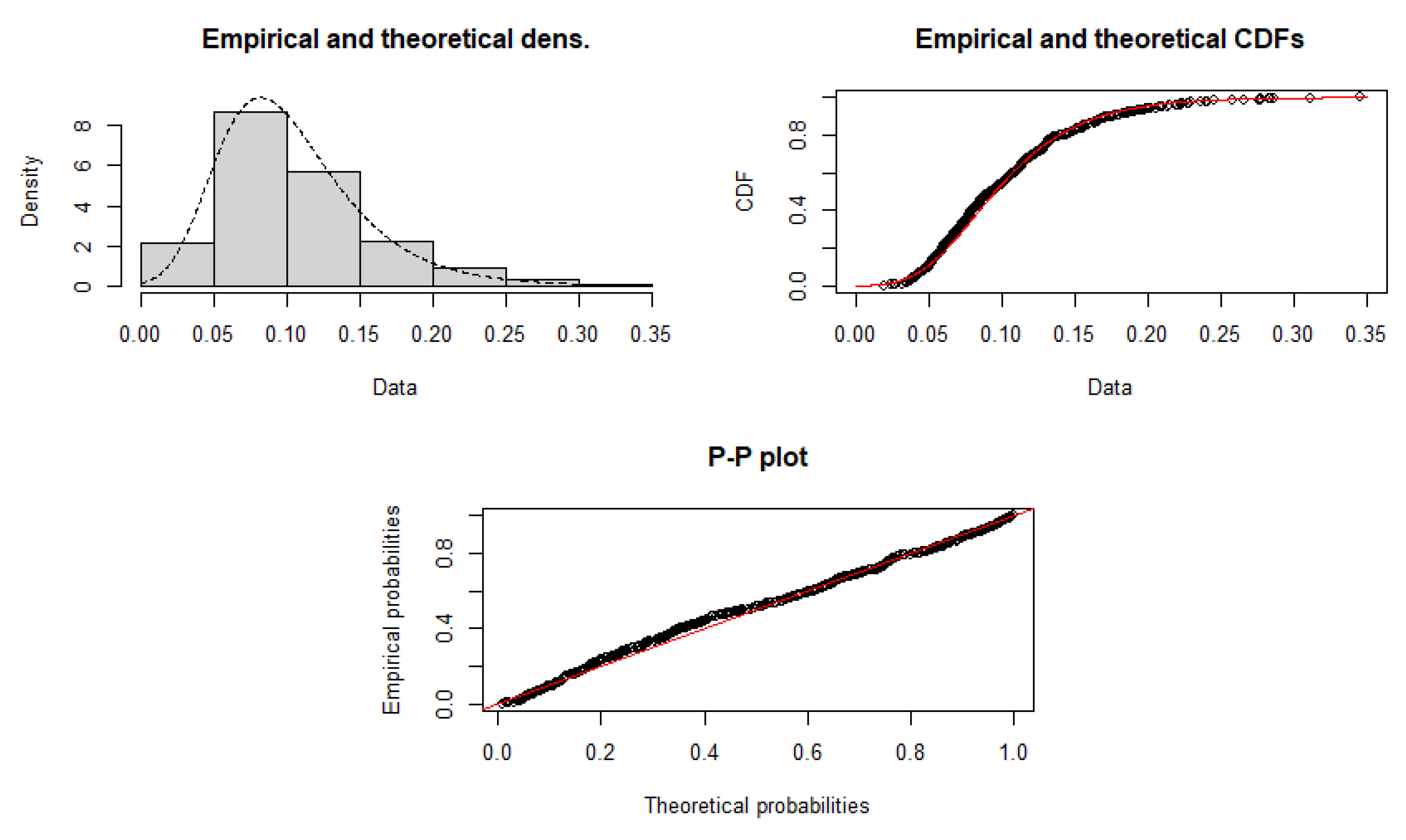
3.2.1. Diagnostic Wisconsin Breast Cancer Data

The two datasets are part of the Diagnostic Wisconsin Breast Cancer Data, which describe some characteristics of the cell nuclei presented in a digitized image of a fine needle aspirate of a breast mass. The dataset was collected and made open by Wolberg et al. at the University of Wisconsin. These data were first used in [31], and they are available at the UC Irvine Machine Learning Repository [32].
The Diagnostic Wisconsin Breast Cancer Data contain 30 features (V3, V4,..., V32) for each cell nucleus. The MAPE model is applied to V8 and V14. Table 5 and Table 6 provide, for V8 and V14, respectively, the MLEs of the parameters of all models and the statistics: minus maximized log-likelihood function, AIC, BIC, HQIC, KS and p-values. It is clear that whereas the exponential distribution failed to fit the data, the MAPE distribution succeeded. It fitted the two datasets with the lowest values of the minus maximized log-likelihood, AIC, BIC, HQIC and KS statistics, as well as the largest 
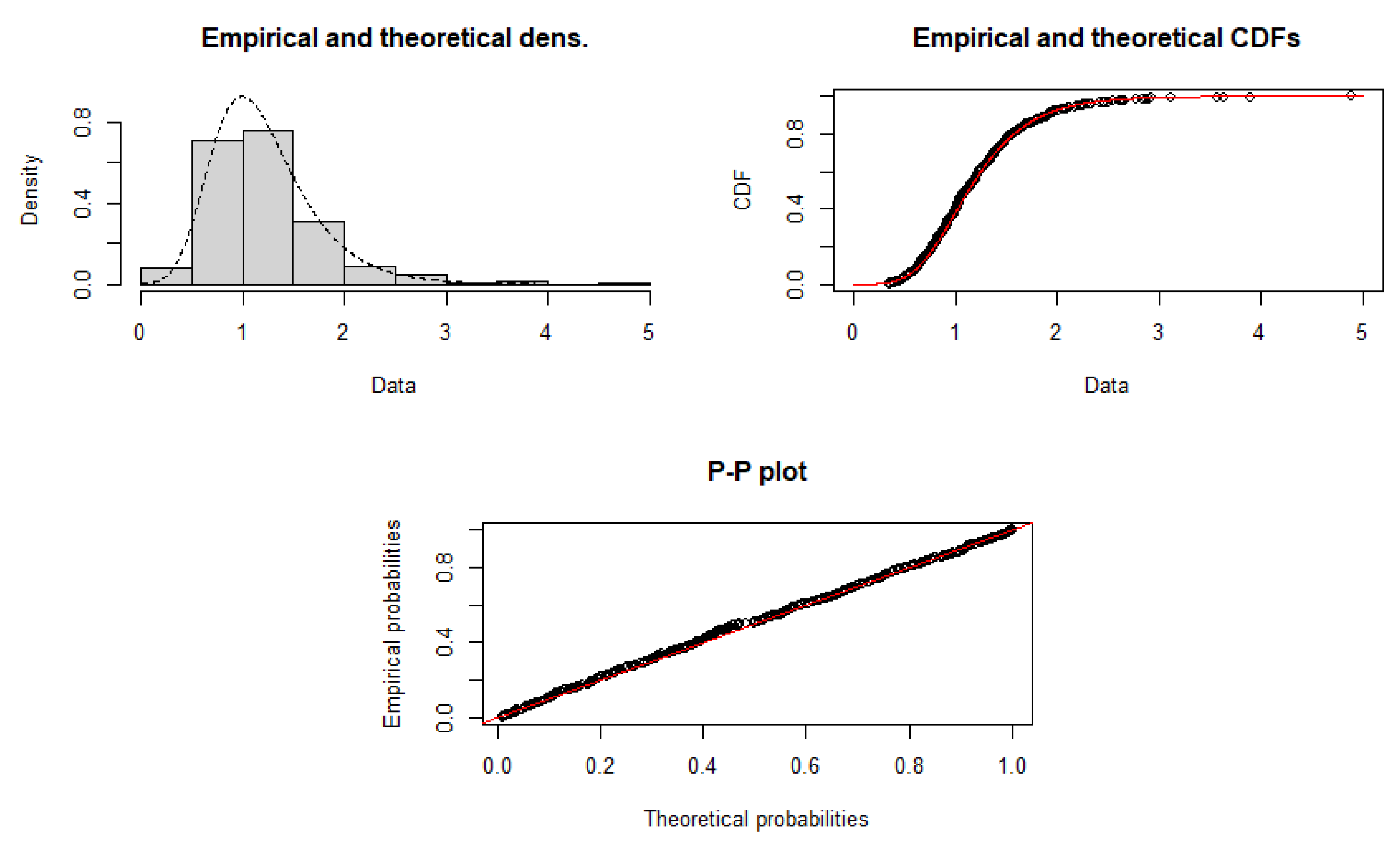
p-values among all models. Thus, it is revealed to be the best model for these data. To compare the empirical distribution of the data with the MAPE distribution, Figure 4 and Figure 5 display: (a) a relative histogram and fitted MAPE distribution, (b) plots of the fitted MAPE survival function and the empirical survival and (c) a probability vs. probability (P-P) plot, respectively. These plots support the results reported in Table 5 and Table 6.

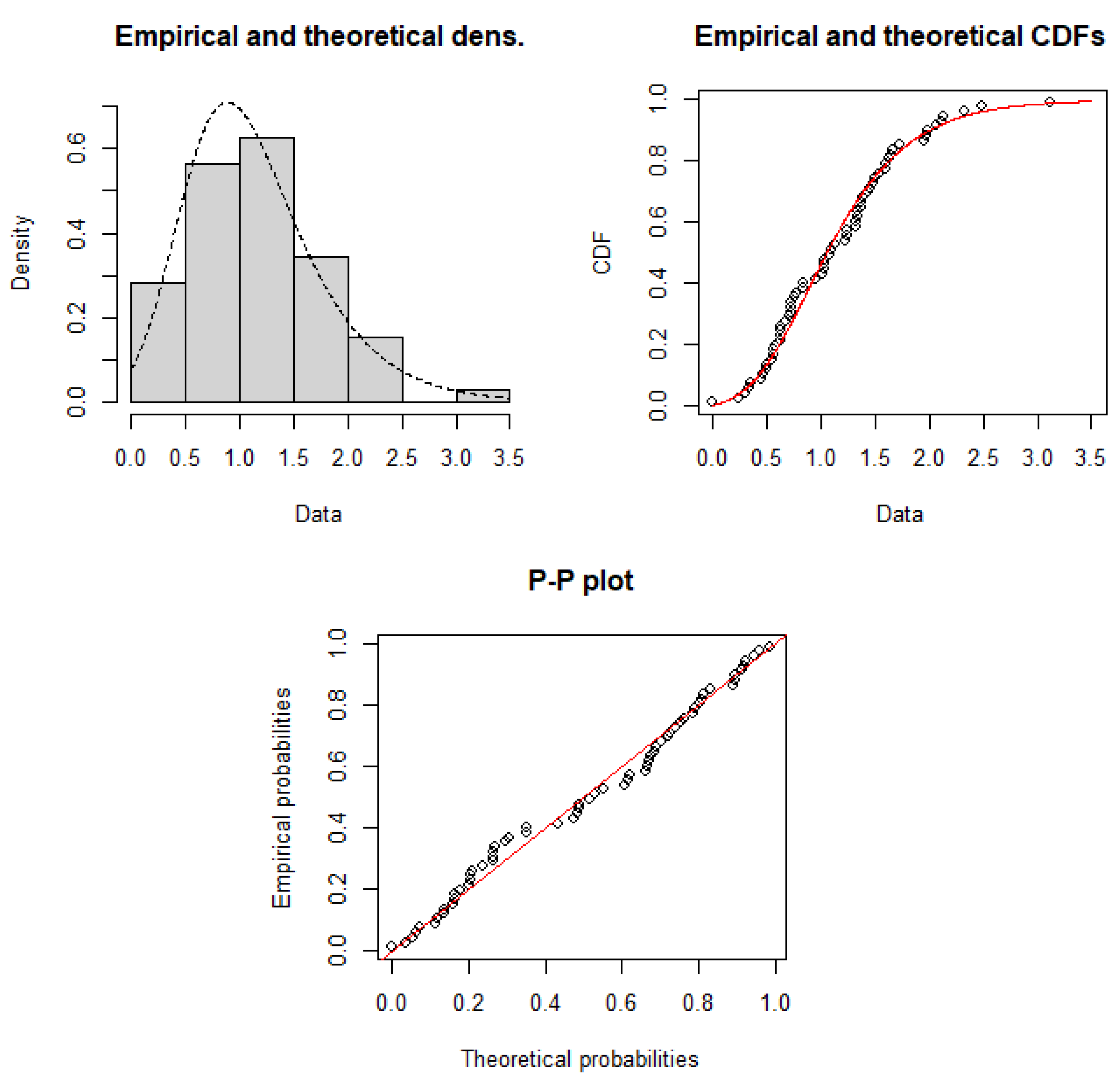
3.2.2. Failure Stress of Carbon Fibers

The dataset refers to the failure stresses (in GPa) of 64 bundles of carbon fibres [33] which were also analyzed in [34] using LET-F family. We transform the recorded failure stresses (x) using the transformation y = x m i n ( x ) . The observations are:
0.000, 0.231, 0.302, 0.327, 0.356, 0.449, 0.460, 0.495, 0.496, 0.544, 0.553, 0.553, 0.573, 0.617, 0.621, 0.624, 0.631, 0.674, 0.713, 0.715, 0.717, 0.723, 0.758, 0.774, 0.837, 0.839, 0.955, 1.016, 1.027, 1.036, 1.036, 1.076, 1.095, 1.129, 1.224, 1.238, 1.244, 1.319, 1.322, 1.334, 1.342, 1.363, 1.371, 1.393, 1.431, 1.445, 1.476, 1.507, 1.534, 1.592, 1.600, 1.636, 1.653, 1.661, 1.727, 1.951, 1.970, 1.985, 2.070, 2.123, 2.126, 2.324, 2.494 and 3.119.
Table 7 provides the MLEs of the parameters of the models and the above statistics. Clearly, the MAPE model fitted the data with the largest p-value among all fitted models and smaller KS Statistics, as well as minimum values of the maximized log-likelihood, AIC, BIC and HQIC. Figure 6 supports the results reported in Table 7.

4. Conclusions

Over the last few decades, many generators have been proposed in different areas of data analysis. We presented a new class of distributions with two extra shape parameters called the modified alpha power (MAP) family, which can be a competitive model to well-known classes such as beta-G in [28] and Kumaraswamy-G in [29], among others. Some properties of the new family can be easily found from a linear representation of its density function. We defined an extended exponential distribution. Some of its mathematical properties and the maximum likelihood estimates are reported. The flexibility of an extended exponential distribution in this family is proved empirically by means of three real datasets. Future research can be conducted for other properties and applications.

Author Contributions

Conceptualization, M.H. and G.M.C.; methodology, M.H.; software, M.H.; validation, H.E.; formal analysis, M.H.; investigation, H.E.; data curation, H.E.; writing—original draft preparation, H.E.; writing—review and editing, G.M.C. and M.H. All authors have read and agreed to the published version of the manuscript.

Funding

This research received no external funding.

Institutional Review Board Statement

Not applicable.

Informed Consent Statement

Not applicable.

Data Availability Statement

Publicly available datasets were analyzed in this study. This data can be found at UCI Machine Learning Repository (accessed 31 October 2021): http://archive.ics.uci.edu/ml.

Conflicts of Interest

The authors declare no conflict of interest.

Abbreviations

The following abbreviations are used in this manuscript:
AICAkaike information criterion
APalpha power
APEalpha power exponential
BICBayesian information criterion
cdfcumulative distribution function
HQICHannan–Quinn information criterion
HRFhazard rate function
KSKolmogorov–Smirnov
MAPmodified alpha power
MAPEmodified alpha power exponential
MLEmaximum likelihood estimate
MOEMarshall–Olkin exponential distribution
P-Pprobability vs. probability
pdfprobability distribution function

Appendix A

By using the power series
β F 2 x = β 1 + e 2 λ x 2 e λ x = β i , j = 0 2 j ln β i + j e λ x ( 2 i + j ) i ! j !
and
α F x = α ( 1 e λ x ) = α k = 0 ln α k e k λ x k ! ,
we obtain
μ r = α β λ α β 1 ln α i , j , k = 0 ψ i , j , k I 1 + 2 ln β i , j , k = 0 ψ i , j , k I 2 ,
where
I 1 = 0 x r e 2 i + j + k + 1 λ x d x = r ! λ r + 1 η i , j , k ,
I 2 = 0 x r e 2 i + j + k + 1 λ x 1 e λ x d x = r ! λ r + 1 η i , j , k r ! λ r + 1 η i , j , k + 1 ,
ψ i , j , k = 2 j ln β i + j ln α k i ! j ! k ! ,
and
η i , j , k = 1 2 i + j + k + 1 r + 1 .
Substituting for I 1 and I 2 , we have
μ r = r ! α β λ r ( α β 1 ) ln α i , j , k = 0 ψ i , j , k η i , j , k + 2 ln β k = 0 ψ i , j , k η i , j , k η i , j , k + 1 .

References

  1. Ahuja, J.C.; Nash, S.W. The Generalized Gompertz-Verhulst Family of Distributions. Sankhyā Indian J. Stat. Ser. A 1967, 29, 1961–2002. [Google Scholar]
  2. Gupta, R.C.; Gupta, R.D. Proportional Reversed Hazard Rate Model and Its Applications. J. Stat. Plan. Inference 2007, 137, 3525–3536. [Google Scholar] [CrossRef]
  3. Lehmann, E.L. The Power of Rank Tests. Ann. Math. Stat. 1953, 24, 23–43. [Google Scholar] [CrossRef]
  4. Azzalini, A. A Class of Distributions Which Includes the Normal Ones. Scand. J. Stat. 1985, 12, 171–178. [Google Scholar]
  5. Marshall, A.W.; Olkin, I. A New Method for Adding a Parameter to a Family of Distributions with Application to the Exponential and Weibull Families. Biometrika 1997, 84, 641–652. [Google Scholar] [CrossRef]
  6. Al-Hussaini, E.K.; Ghitany, M.E. On Certain Countable Mixtures of Absolutely Continuous Distributions. Metron 2005, 63, 39–53. [Google Scholar]
  7. Barakat, H.M. A New Method for Adding Two Parameters to a Family of Distributions with Application to the Normal and Exponential Families. Stat. Methods Appl. 2015, 24, 359–372. [Google Scholar] [CrossRef]
  8. Mahdavi, A.; Kundu, D. A New Method for Generating Distributions with an Application to Exponential Distribution. Commun. Stat.-Theory Methods 2017, 46, 6543–6557. [Google Scholar] [CrossRef]
  9. Nassar, M.; Alzaatreh, A.; Mead, M.; Abo-Kasem, O. Alpha Power Weibull Distribution: Properties and Applications. Commun. Stat.-Theory Methods 2017, 46, 10236–10252. [Google Scholar] [CrossRef]
  10. Ramadan, D.A.; Magdy, W. On the Alpha-Power Inverse Weibull Distribution. Int. J. Comput. Appl. 2018, 181, 6–12. [Google Scholar] [CrossRef]
  11. Dey, S.; Ghosh, I.; Kumar, D. Alpha-Power Transformed Lindley Distribution: Properties and Associated Inference with Application to Earthquake Data. Ann. Data Sci. 2019, 6, 623–650. [Google Scholar] [CrossRef]
  12. Ihtisham, S.; Khalil, A.; Manzoor, S.; Khan, S.A.; Ali, A. Alpha-Power Pareto Distribution: Its Properties and Applications. PLoS ONE 2019, 14, e0218027. [Google Scholar] [CrossRef] [PubMed]
  13. Ahmed, M.A. On the Alpha Power Kumaraswamy Distribution: Properties, Simulation and Application. Rev. Colomb. Estad. 2020, 43, 285–313. [Google Scholar] [CrossRef]
  14. Eghwerido, J.T.; Nzei, L.C.; Agu, F.I. The Alpha Power Gompertz Distribution: Characterization, Properties, and Applications. Sankhya A 2021, 83, 449–475. [Google Scholar] [CrossRef]
  15. Hassan, A.S.; Mohamd, R.E.; Elgarhy, M.; Fayomi, A. Alpha Power Transformed Extended Exponential Distribution: Properties and Applications. J. Nonlinear Sci. Appl. 2018, 12, 62–67. [Google Scholar] [CrossRef] [Green Version]
  16. Ahmad, Z.; Ilyas, M.; Hamedani, G.G. The Extended Alpha Power Transformed Family of Distributions: Properties and Applications. J. Data Sci. 2021, 17, 726–741. [Google Scholar] [CrossRef]
  17. Bantan, R.; Elsehetry, M.; Hassan, A.S.; Elgarhy, M.; Sharma, D.; Chesneau, C.; Jamal, F. A Two-Parameter Model: Properties and Estimation under Ranked Sampling. Mathematics 2021, 9, 1214. [Google Scholar] [CrossRef]
  18. Patil, G.P. Weighted Distributions. In Wiley StatsRef: Statistics Reference Online; Wiley: Hoboken, NJ, USA, 2014. [Google Scholar]
  19. Tahir, M.H.; Nadarajah, S. Parameter induction in continuous univariate distributions: Well-established G families. An. Acad. Bras. Ciênc 2015, 87, 539–568. [Google Scholar] [CrossRef]
  20. Piessens, R.; de Doncker-Kapenga, E.; Überhuber, C.W.; Kahaner, D.K. Guidelines for the Use of QUADPACK. In Springer Series in Computational Mathematics; Springer: Berlin/Heidelberg, Germany, 1983. [Google Scholar]
  21. AL-Hussaini, E.K.; Hussein, M. Estimation under a Finite Mixture of Exponentiated Exponential Components Model and Balanced Square Error Loss. Open J. Stat. 2012, 2, 1. [Google Scholar] [CrossRef] [Green Version]
  22. Flury, B.D. Acceptance—Rejection Sampling Made Easy. SIAM Rev. 1990, 32, 474–476. [Google Scholar] [CrossRef]
  23. Kennedy, J.; Eberhart, R.C. Particle swarm optimization. In Proceedings of the IEEE International Conference on Neural Networks, Perth, Australia, 27 November–1 December 1995; pp. 1942–1948. [Google Scholar]
  24. R Core Team. R: A Language and Environment for Statistical Computing; R Foundation for Statistical Computing: Vienna, Austria, 2020. [Google Scholar]
  25. Steinbrecher, G. Taylor Expansion for Inverse Error Function Around Origin; Working Paper; University of Craiova: Craiova, Romania, 2002. [Google Scholar]
  26. Nadarajah, S.; Rocha, R. Newdistns: An R Package for New Families of Distributions. J. Stat. Softw. 2016, 69, 1–32. [Google Scholar] [CrossRef] [Green Version]
  27. Jones, M.C.; Pewsey, A. Sinh-arcsinh distributions. Biometrika 2009, 96, 761–780. [Google Scholar] [CrossRef] [Green Version]
  28. Eugene, N.; Lee, C.; Famoye, F. Beta-Normal Distribution and Its Applications. Commun. Stat.-Theory Methods 2002, 31, 497–512. [Google Scholar] [CrossRef]
  29. Cordeiro, G.M.; de Castro, M. A new family of generalized distributions. J. Stat. Comput. Simul. 2011, 81, 883–898. [Google Scholar] [CrossRef]
  30. Delignette-Muller, M.L.; Dutang, C. Fitdistrplus: An R Package for Fitting Distributions. J. Stat. Softw. 2015, 64, 1–34. [Google Scholar] [CrossRef] [Green Version]
  31. Street, W.N.; Wolberg, W.H.; Mangasarian, O.L. Nuclear Feature Extraction for Breast Tumor Diagnosis. Proc. Biomed. Image Process. Biomed. Vis. 1993, 1905, 861–870. [Google Scholar]
  32. Wolberg, W.H.; Street, W.N.; Olvi, L. Mangasarian UCI Machine Learning Repository. Available online: http://archive.ics.uci.edu/ml (accessed on 12 September 2021).
  33. Cheng, R.C.; Traylor, L. Characterization of material strength properties using probabilistic mixture models. WIT Trans. Model. Simul. 1970, 31, 553–560. [Google Scholar]
  34. Aslam, M.; Ley, C.; Hussain, Z.; Shah, S.F.; Asghar, Z. A new generator for proposing flexible lifetime distributions and its properties. PLoS ONE 2020, 15, e0231908. [Google Scholar] [CrossRef]
Figure 1. The effects of α and β on the cdfs of the exponential (a,b), Weibull (c,d) and normal (e,f) distributions.
Symmetry 14 00276 g001
Figure 2. The effects of α and β on the pdfs of the exponential (a,b), Weibull (c,d) and normal (e,f) distributions.
Symmetry 14 00276 g002
Figure 3. The effects of α and β on the hrfs of the exponential (a,b) and Weibull (c,d) distributions.
Symmetry 14 00276 g003
Figure 4. Empirical density, empirical cdf and P-P plot of the fitted MAPE distribution to V8.
Symmetry 14 00276 g004
Figure 5. Empirical density, empirical cdf and P-P plot of the fitted MAPE distribution to V14.
Symmetry 14 00276 g005
Figure 6. Empirical density, empirical cdf and P-P plot of the fitted MAPE distribution to failure stress data.
Symmetry 14 00276 g006
Table 1. Statistics for the MAPE distribution for some parameter values.
λ α β μ 1 μ 2 Var ( X ) SkewnessKurtosisMode Q 1 Median Q 3
0.11.1110.2395207.219102.3721.964758.7909502.998587.1725414.221
0.2239.17665123.62839.41721.267395.639065.817144.578637.9977712.4161
0.531.53.1144215.48745.787761.420556.159691.435231.328262.590544.30670
1452.125606.198671.680511.141735.291791.557451.194971.913732.81104
2220.827051.057220.373211.364775.962560.443420.375690.700741.13450
Table 2. Simulation findings.
α ^ β ^ λ ^
n AverageABMSEAverageABMSEAverageABMSE
502.65190.34810.53951.94050.05950.01771.64550.35450.0427
α = 3 1002.69130.30870.22581.95210.04790.01511.88230.11770.0311
β = 2 1503.15200.15200.09261.95670.04330.01441.89390.10610.0217
λ = 2 2003.04720.04720.09121.95820.04180.01331.89520.10480.0205
2503.04080.04080.08921.96670.03330.01041.89730.10270.0195
503.20850.20850.42491.23410.76590.59960.27720.22280.0549
α = 3 1002.80720.19280.24842.34680.34680.52180.32310.17690.0360
β = 2 1502.82040.17960.20412.14260.14260.43210.32960.17040.0329
λ = 0.5 2002.87670.12330.12671.89230.10770.40700.40590.09410.0122
2503.01340.01340.07941.92690.07310.39130.40810.09190.0092
502.04670.95330.98761.96240.96240.98830.79840.20160.0675
α = 3 1002.10310.89690.92651.95030.95030.94171.14210.14210.0362
β = 1 1503.46610.46610.26151.27800.27800.10181.10700.10700.0312
λ = 1 2003.16020.16020.13231.20600.20600.06131.05740.05740.0101
2503.09990.09990.11521.10930.10930.01761.03600.03600.0088
503.09150.59150.94282.24710.25290.57660.54670.15330.0260
α = 2.5 1002.81790.31790.45822.26790.23210.53390.55700.14300.0255
β = 0.5 1502.78160.28160.44372.32690.17310.38220.58020.11980.0176
λ = 0.7 2002.32230.17770.21182.39270.10730.23780.58350.11650.0146
2502.44090.05910.03402.53910.03910.03840.68590.01410.0143
501.95131.54872.40172.05660.95660.91810.82390.07610.0180
α = 3.5 1003.21200.28800.46561.25400.15400.16610.93970.03970.0174
β = 1.1 1503.27510.22490.14721.19740.09740.02430.86940.03060.0144
λ = 0.9 2003.44610.05390.06171.08030.01970.00610.92170.02170.0046
2503.53300.03300.03241.09650.00350.00360.88250.01750.0032
502.02780.17220.04631.94970.25030.07371.85850.14150.0437
α = 2.2 1002.02920.17080.04031.95880.24120.06821.89340.10660.0217
β = 2.2 1502.04190.15810.03881.96470.23530.06771.89340.10660.0217
λ = 2 2002.04450.15550.03581.97350.22650.05851.89600.10400.0202
2502.05390.14610.03561.97520.22480.05771.89680.10320.0197
Table 3. Results for the simulated MAPE data.
α ^ β ^ λ ^ Minus Log-LikelihoodAICBICHQICKS StatisticKS p-Value
MAPE1.61611.87500.4688216.4997438.9995446.8150442.16250.04000.999998
Beta-E1.47706.07540.0685218.9210443.8421451.6576447.00510.05370.935500
Kw-E1.359916.92710.0355217.7373441.4745449.2901444.63760.04890.970400
MOE3.49430.5118-218.9981441.9962447.2065443.30490.04060.996526
Table 4. Results for the simulated MAPN data.
Minus Log-LikelihoodAICBICHQICKS StatisticKS p-Value
MAPN α ^ = 8.9431 β ^ = 14.9992118.7269241.4538246.6642243.56260.050.9996
Normal μ ^ = 1.3407 σ ^ = 0.8069120.4394244.8789250.0892246.98760.090.8127
SAS ϵ ^ = −0.8774 δ ^ = 1.1704149.7595303.5189308.7293305.62760.33 3.73 × 10 5
Table 5. MLEs and goodness of fit statistics for V8.
Distribution λ ^ α ^ β ^ Minus Log-LikelihoodAICBICHQICKS Statisticp-Value
Exponential9.58396--−716.9918−1431.99−1427.6−1430.30.279442.2 × 10 16
Weibull0.118332.1092-−914.7481−1825.50−1816.8−1822.10.066780.158
APE0.46448 5.8 × 10 10 -−706.5671−1409.13−1400.4−1405.70.284712.2 × 10 16
MOE31.285920.2769-−902.5504−1801.10−1801.1−1797.70.074750.0035
MAPE26.0899297.03633.9260-937.1483−1868.30−1855.3−1863.20.050970.4508
Table 6. MLEs and goodness of fit statistics for V14.
Distribution λ ^ α ^ β ^ Minus Log-LikelihoodAICBICHQICKS Statisticp-Value
Exponential0.8218--680.67671363.3531367.6971365.0480.316342.2 × 10 16
Weibull1.37502.3027-433.8886871.7772880.465875.16720.0738140.09007
APE2.12631609.99-401.5559807.1118815.800810.50180.0544820.3671
MOE3.266742.5702-423.8381851.6763860.364855.06630.0591950.0371
MAPE2.5742136.600953.2925387.8032781.6064794.638786.69130.0333920.9089
Table 7. MLEs and goodness of fit statistics for the failure stress data.
α ^ β ^ λ ^ Minus Log-LikelihoodAICBICHQICKS StatisticKS p-Value
MAPE7.49686.76982.012856.6248119.2495125.7262121.80100.07810.9898
Beta-E39.72494.15640.810057.2210120.4420126.9186122.99350.08760.7093
Kw-E67.67311.87101.363857.0680120.1361126.6127122.68760.08610.7298
Publisher’s Note: MDPI stays neutral with regard to jurisdictional claims in published maps and institutional affiliations.

