Abstract
The real-time control of optimal power flow (OPF) in electric networks represents, in the last period, a challenge for the Distribution Network Operators (DNOs) and Transmission System Operators (TSOs) under the conditions of large-scale integration of renewable energy sources. The paper focused on the voltage management in the electric networks with wind farms connected, proposing a fast Successive Quadratic Programming (SQP)-based centralized control (CC) methodology of the on-load tap changers (OLTC) corresponding to the transformers from the electric substations, which can be included in the Optimal Power Flow (OPF) module of the Supervisory Control and Data Acquisition (SCADA) Master System. The SQP-CC aims to ensure an optimal voltage level inside a variation range, as narrow as possible, which leads to minimize power losses in the electric networks. Treating the OPF problem as an SQP problem and accelerating convergence using the conjugate reduced gradient method led to very few iterations and a fast computational time, recommending the implementation of the methodology for real-time work. The effectiveness of the SQP-CC was demonstrated in a test network having two voltage levels (220 and 110 kV) with two wind farms integrated, considering two scenarios, without and with wind farms connected. The optimal tap positions of the transformers led to very close voltage variations between the buses of the network, quantified through an average voltage drop between the initial and final buses by 0.004 pu compared with 0.031 pu recorded in the scenario with both wind farms injecting power into the network and without coordinated control of the OLTCs. The energy-saving was over 30% in both scenarios, 33.5% (without wind farms) and 41.27% (both wind farms injecting power in the network). These results highlighted the positive effects of the proposed SQP-CC methodology on the real-time optimal operation of the electric networks integrating wind farms.
1. Introduction
Using renewable energy as clean energy globally represents one of the main objectives of global energy policy that, in the context of sustainable development, aims to decrease fossil fuel consumption, reduce greenhouse gas emissions, and discover new viable technologies for energy production.
Following the European Union (EU)’s accession to the Paris Agreement [1] and the publication of the Energy Union Strategy, the EU has taken on a significant role in combating climate change through its five leading dimensions: energy security, decarbonization, energy efficiency, the internal energy market and research, innovation and competitiveness [2]. Renewable energy sources (wind energy, solar energy, hydropower, ocean energy, geothermal energy, biomass, and biofuels) are alternatives to fossil fuels that help to reduce greenhouse gas emissions, diversify energy supply, and reduce dependence on the volatile and uncertain markets for fossil fuels, especially oil and gas. EU legislation regarding the promotion of renewable sources has evolved significantly over the last 15 years. To meet this commitment, the EU has set the following energy and climate targets for 2030 [1,2]:
- reducing greenhouse gas emissions by at least 40% compared to 1990;
- the consumption of renewable energy to be 32%;
- improving energy efficiency by 32.5%;
- interconnecting the electricity market at a level of 15%.
To guarantee the achievement of these objectives, each member state has a National Energy and Climate Plan (NECP) for the period 2021–2030. The NECP projects set the objectives and national contributions to achieving EU climate change goals. The targets in the NECPs associated with each member state are presented in Figure 1 [3].
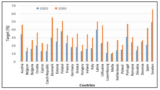
Figure 1.
Comparison between the targets of the UE member states from 2020 and 2030 included in the NECPs [3].
The differences between the two targets assumed by each country are significant, 1.5% (Malta) and 25% (Denmark), the UE average value is 12.2%. Austria, Cyprus, Greece, and Poland have indicated in the figure the minimum values of the target, but they fixed themselves and maximum values, which could be achieved depending on different technical, economic, and policy factors.
Important funding options to combat the effects of climate change will be available for each country in the coming years. These will be focused mainly on increasing the number of renewable energy sources and improving the energy efficiency to reduce greenhouse gas emissions. For example, within the EU budget for the 2021–2027 period, Romania can access over 6 billion EUR through European funds for sustainable development and fair transition and more than 30 billion EUR through the recovery and resilience facility [4]. Another significant source of funding is the Emissions Trading Scheme (EU ETS), of which Romania can obtain revenues from auctions estimated at over 15 billion EUR between 2020 and 2030. An increase of renewable sources in Romania requires investments of at least EUR 22 billion by 2030 according to NECP [5] and, to achieve a fair transition, a necessary budget of around EUR 0.7 billion is expected [6]. Additional investments are needed to reach a carbon-neutral energy system by 2050.
Considering the constraints related to renewable sources associated with their fluctuating nature, it is clear that the power system cannot widely integrate these technologies without the need to invest in the electric distribution and transmission networks and, also, in the storage systems. The distribution of wind potential allows the capitalization of high economic performance for a few geographical regions where there is a concentration of wind capacities, causing an overload of the transmission and distribution networks. The emergence of renewable energy technologies led to efficient solutions regarding the new production capacities integrated close to the resource and not to the consumption zone. In other words, this means that the networks must be flexible, providing an optimal integration. In the first stage, these solutions should consider areas with high potential, and the investments in the networks to be done in the second stage [7].
Thus, a renewable energy resource map can provide detailed information on the real potential of each area. After that, the Decision-Maker (DM) must evaluate if it is necessary to make investments in networks to evacuate the energy injected by these sources. Once the connection costs are optimized, the renewables no longer need subsidies. However, the market rules should adapt to the new conditions and efficient management of the networks. These must be digitized, ensuring the flexibility of the networks [7,8].
Due to these targets, the number of wind farms has increased in recent years, such that the Distribution Network Operators (DNOs) and Transmission System Operators (TSOs) need to carry out analyses for evaluating their impact on the network operation. These analyses aim to identify the optimal power flow (OPF) considering the power injections of wind farms. Figure 2 displays the impact of wind farms integrated into the electric networks, depending on the time horizon and width of the area considered in the analyses [9,10].
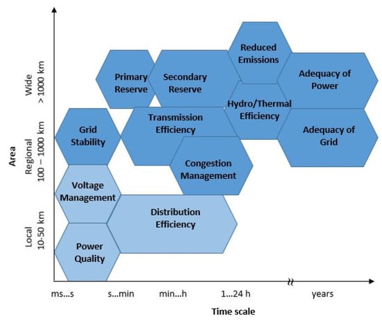
Figure 2.
The impacts of wind farms integrated into the electric networks, divided into different time scales and width of the area relevant for the analyses.
The time scales utilized in the impact studies of the wind farms on the electrical networks lead to a variety of the proposed models. These impact studies evaluated the following technical problems depending on the width of the area: reserve/regulating power (time/minute to half an hour), efficiency/unit commitment (time/hours to days) associated with the wind power forecasting, adequacy of power (having years as the time horizon), adequacy of the transmission networks (time/hours to years), grid stability (time/seconds to minutes), voltage management (time/seconds to minutes), and power quality (time/milliseconds to minutes).
The paper focuses on voltage management, particularly voltage control in the electric networks with wind farms connected, proposing an original centralized control methodology (integrated into the Optimal Power Flow (OPF) module of the SCADA master system from the Central Dispatch) of the on-load tap changers (OLTC) corresponding to the transformers from the electric substations. SCADA is an acronym associated with Supervisory Control and Data Acquisition. Regarding the SCADA master system from the Central Dispatch of the DNOs or TSOs, it performs centralized monitoring and control for the electric networks over long-distance communications networks, including monitoring alarms and processing status data [11]. The main components refer to a central computer, operator interfaces, mass data storage, control software, and integrated communication networks. At the local level of the electric substations, there are peripherals suitable for real-time supervisory and control. In the control room of each substation, the system contains at least a Remote Terminal Unit (RTU), Station Master, having the functions of a data concentrator, real-time data server, and communication server. The SCADA system of the wind farms allows complete remote control and supervision of the entire wind farm and the individual wind turbines [12]. This works like a brain, connecting the individual turbines, the electric substation, and meteorological stations to a central data concentrator, CDC (master computer), which, together with a high communication network, enables the DM to supervise the behavior of all the wind turbines and, also, the wind farm [13]. The sensors for wind speed, wind direction, shaft rotation speed, and numerous other factors take over and communicate data to the CDC [14]. It will record in the database all the activity (with various sampling steps, 5 to 60 min, depending on the programming) and allows the operator to decide what corrective action (if it is necessary) is required to maximize the injected power [15]. Under these conditions, the changes in wind generation are managed within the SCADA system. Towards the central master SCADA system of the DNO or TSO, the injected power, daily energy, availability, and error signals are sent at equal time intervals (equal to the sampling step) [13,15], serving as the basis for the real-time OPF calculations based on the proposed coordinated control methodology.
The assumptions considered by the authors to integrate the proposed methodology in the OPF module referred to the use of the data uploaded from the SCADA systems implemented in the electric substations and the wind farms. These data from the two SCADA systems are transmitted through a wide-area communication network with high-speed data transmission in real-time to the SCADA master system from the Central Dispatch. At this level, only data associated with the load (active and reactive powers) of each substation and the power injection by each wind farm, uploaded in real-time from the SCADA systems, will represent the input data for the OPF module that manages the OLTC of the transformer by simultaneous commands based on the proposed methodology. Regarding the changes in the wind generation, these are managed within the SCADA system implemented at the wind farm level, as presented above, and only the data sent to the SCADA master system are used by the methodology, see Figure 3. The methodology has, as the starting point, the ability of the TSOs and DNOs to hold the control capability of the transformers due to the advanced technologies based on the automatic voltage control (AVC). It can be integrated considering both operation modes (real-time and off-line). The real-time implementation requests the technical features relating to a wide-area communication network with high-speed data transmission [16], an OPF module with a fast processing speed [17], and the OLTC of the transformer to perform quick changing of the taps [18,19].
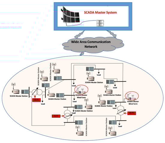
Figure 3.
The architecture of the SCADA system from the electric networks integrating wind farms.
1.1. Related Literature
Different optimization methods for the steady-state of the electrical networks (called, also, Optimal Power Flow—OPF) for integrating the renewable energy sources have been proposed.
Some studies considered the mathematical models to determine the optimal solution using classical optimization methods [20,21,22,23]. A techno-economic analysis of the influence of grid regulation, including the aspects regarding the bilateral power agreements between the power producers, the Norwegian power market, and system conditions, is presented in [20]. The authors investigated the optimal utilization of the grid capacity considering a high penetration level of wind energy in a power system with more hydropower plants. The optimal operation has been obtained considering the minimization of wind curtailment and hydro reservoir spillage using linear programming. Leon et al. used the constrained quadratic programming in [21] to solve the contingency-constrained OPF in the electric networks considering only photovoltaic generation. Hmida et al. improved the convergence of the quadratic programming using an imperialist competitive algorithm in [22]. Various IEEE test systems have been used to demonstrate the accuracy of the proposed approach. Zhifang et al. [23] proposed the linear approximation of power flow equations to reduce the number of iterations in the OPF process. The authors used the IEEE and Polish systems to test and validate the accuracy of the proposed OPF algorithm. Moreover, the meta-heuristic optimization techniques have been used by researchers to solve the OPF problem in the electric networks integrating wind farms. Alham et al. addressed in [24] the dynamic economic dispatch based on demand-side management using a genetic algorithm in an electric network with six wind farms. A weak point of this approach is the lack of technical constraints in the mathematical model.
Khamees et al., in [25], considered stochastic modeling with the objective of obtaining an optimal schedule of the wind farms and thermal power plants. The economic quantification is performed finally through the total operation cost. An algorithm from the metaheuristic optimization category (the Aquila optimizer) determined the optimal solution in the cases of the IEEE-30, IEEE-57, and IEEE-118 buses test systems. Shi et al. analyzed, in [26], a multi-objective optimal dispatch model considering simultaneous minimization of both operational cost and power loss. The solution has been obtained based on the quantum particle swarm optimization (PSO) for the IEEE-30 bus test system. An improved PSO algorithm-based approach proposed, in [27], by Duy and Loc tried to solve the optimal operation problem of a hybrid power system with solar and wind energy sources. The approach has been tested in the IEEE-30 bus test system. Balaban et al. analyzed [28] the operation of an area of the Romanian power system, characterized by a high density of wind farms, which included the voltage levels, overloading of power system elements, and the transient stability conditions of classic and wind power plants. The optimal power flow was solved by Mishra et al. [29] in the presence of the wind farms with an optimization technique of a modified cuckoo search in the cases of IEEE 30 and IEEE 57-bus test systems. The weaknesses of this approach refer to the lack of load variations and changes in the market.
The Ant Lion Optimizer has been applied by Kouadri et al. [30] to minimize the total generation cost of the thermal power plants and wind farms in the electric networks with high-voltage DC converters. The authors used the IEEE 30-bus system to test the proposed approach.
The most efficient classical approaches based on the gradient methods are presented in [31,32,33]. Inoue et al. proposed [31] the gradient descent algorithm in the OPF design to solve two problems from a power system: minimize the fuel cost and improve the dynamic performance. The efficiency of the approach has been verified in the 68-bus test system integrating a solar farm. Gan used [32] a variant of the gradient algorithm that works online with the OPF problem from the radial electric networks. The algorithm has been tested in various networks having a computational time between 0.27 and 2.35 s. An approach based on the reduced gradient method combined with the augmented Lagrangian method with barriers has been applied by Carvalho in [33]. The results obtained in the case of the IEEE 30-bus system highlighted a reduced number of iterations (six iterations).
Table 1 presents a synthesis of some representative approaches proposed in the literature after 2015, highlighting the treated topic, the contributions, and the proposed optimization method.

Table 1.
Synthesis of the approaches proposed in the literature.
The comparison based on the number of iterations and computational time highlighted better performances of classical algorithms from the mathematical programming. Thus, if the IEEE-30 bus system is taken as the reference, meta-heuristic algorithms led to a high number of iterations (in the order of hundreds) and a computational time (in the order of minutes): (Cuckoo search—5.75 min [29], particle swarm optimization—5.71 min [29], and Aquila optimizer—11.6 min [25]) compared with the classical mathematical programming (quadratic programming—0.5 s [21] and reduced gradient algorithm—0.27 s [32]). Because the meta-heuristic algorithms have a high computational time, in the order of minutes, their implementation in the OPF module from the SCADA master system to real-time work is not feasible. In these conditions, the classical algorithms can solve, in real-time, the OPF problem in the electric networks integrating the wind farms.
1.2. Main Contributions
Various approaches based on the classical or meta-heuristic methods have been developed in the literature to solve the OPF problem in the electric networks integrating renewable sources. Most of them have not been tested on the real electric networks but in IEEE or adapted networks imposing certain buses in which renewable sources are located and only for an hourly steady-state.
However, a coordinated control methodology that manages the OLTC of the transformers, integrated into the OPF module from the SCADA master system from the Central Dispatch of the DNOs or TSOs, has not been clearly defined in the literature. Thus, the authors proposed the integration framework of an original real-time coordinated control methodology of the OLTCs in a SCADA master system to ensure an optimal voltage level in the electric networks with positive consequences on reducing the power losses.
Compared with the previous approaches, the methodology represents a practical application that ensures the flexibility of the voltage control in the electric networks with and without integrated renewable sources, such as wind farms, by the correlation between the tap positions of the transformers. The main contributions refer to the following:
- Developing a data structure integrated into a real-time query procedure that uploads information from the SCADA master system and saves them in two databases (Topology Database and Profiles Database) accessed by the OPF module. This structure enables high-speed data processing.
- Treating the OPF problem as a successive quadratic programming (SQP) problem and accelerating convergence using the conjugate reduced gradient method. The small number of iterations and the fast computational time represent the strong points and recommend it for real-time work.
- Performing deep research, considering a real network, representing a zone of the Romanian transmission and distribution system, where two scenarios have been analyzed (without and with wind farms connected) to quantify the benefits on the operation of the network with the wind power sources integrated overlapping the coordinated control of the OLTCs. The considered scenarios (together with the three cases analyzed within the second scenario) cover all situations associated with the steady-state of the electrical networks.
The methodology can lead to significant technical and economic benefits in the operation of the electric networks, with and without the renewable sources connected, considering mainly the wind farms, if the requirements regarding the integration of a wide-area communication network with high-speed data transmission, an OPF module with a fast processing speed, and the OLTC of the transformer that performs fast-changing of the taps are met.
1.3. Paper Organization
The paper is organized in the following sections: Section 2 details the components from the structure of the proposed methodology; Section 3 offers a complex analysis performed in a real electric network having two voltage levels (220 and 110 kV) with two wind farms integrated, considering two scenarios, without and with wind farms connected; and Section 4 consists of the conclusions, also accentuating future work.
2. Materials and Methods
The proposed methodology provides the coordinated control of OLTC for all power transformers to achieve an optimal steady-state of the networks, which leads to the minimization of the energy losses. It leads to the best solutions associated with the tap positions of the transformers, taking into account the power injections of the wind farms.
Figure 4 displays the flowchart assigned to the proposed methodology. All necessary data in the control process are available in two databases inside the SCADA Master System, the Topology Database and the Load/Generation Profiles Database.
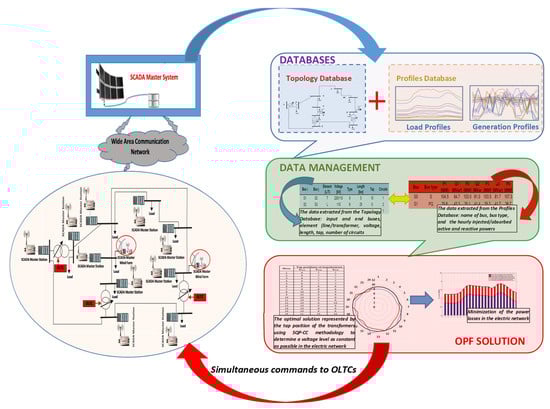
Figure 4.
The flowchart of the proposed coordinated control methodology.
From the databases, the information regarding the technical and location characteristics of the main elements (lines, transformers, classic power plants, and wind farms) from the supervised electric network, and the active/reactive power profiles at the level of the electric substations and wind farms, are uploaded as matrices and vectors. The SQP-based OPF identifies the optimal tap positions of all of the transformers that lead to as constant as possible voltage levels at each bus from the electric network, such that the power losses have the lowest value. Finally, the communication module transmits simultaneously to all OLTCs the new tap positions. The below sections will describe each stage in detail.
2.1. Stage 1. Input Data Management
The methodology is based on a data structure integrated into a real-time query procedure that uploads information from the SCADA master system and saves them in two databases (Topology Database and Profiles Database) accessed by the OPF module. The databases contain the topology recognized through the technical and area characteristics of the main components (buses, conductors, and power transformers) and the power profiles transmitted from the electric substations and those injected by the classical power plants and wind farms. This structure enables high-speed data processing.
2.1.1. Topology Database
The fast recognition of the topology for each electric network from the supervisory and control area of the DNO or TSO represents a strong point for the real-time use of the proposed methodology. All information on the electric substations, the classical power plants, and the wind farms connected to the network through an identification number assigned to the analyzed area by the DM will upload from the Topology Database. A procedure [34] based on a structure containing two vectors, VA and VC, associated with each voltage level, which speeds up the recognition process, is implemented to perform this task. Vector VA records each area of the electric network. Vector VE contains the elements (electric line/power transformer) from each area. The connection between the two voltage levels is done through the elements assigned to the transformers from vector VE associated with the lower voltage level. In the following, the recognized procedure is exemplified using the electric network with two voltage levels (110, blue color, and 220 kV, red color) from Figure 5.
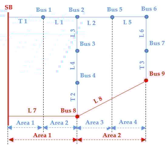
Figure 5.
Exemplification of the recognition procedure in the case of an electric network with two voltage levels (110, blue color, and 220 kV, red color) with 10 buses (including slack bus).
The 110 kV level, having seven buses, is divided into four areas, and the 220 kV level, with three buses, including the slack bus (SB), into two areas. The structure of the two vectors associated with the 110 and 220 kV levels is presented in Table 2.
Table 2.
The structure of the two vectors associated with the two levels.
Thus, the identification of each element, representing the link between each pair of buses, is automatically performed. Moreover, the technical characteristics associated with the transformers with OLTC represent indispensable input data for the methodology.
All this information recorded in the database is uploaded in matrix structures used in the next stage by the control algorithm. Table 3 presents, as an example, such a matrix structure.
Table 3.
A sequence of the matrix structure assigned to the topology data.
The fields have the following signification:
- Bus i, Bus j—represent the two terminals (i—input and j—output) of an element (line or power transformer) associated with the main components (electric substations, the classical power plants, and the wind farms) identified through the numbers in the topology;
- Element—is associated with the power transformer (T) or the line (L) between Bus i and Bus j;
- Voltage—indicated the voltage level, in (kV), for the operation of the Element between Bus i and Bus j;
- Type—is the identification number of the element in the Lines Database or Transformers Database containing the technical specific parameters: rated voltage, resistance, reactance, conductance, susceptance, and the number of tap positions (in the case of the transformers);
- Length—is the length, in (km), when the Element between Bus i and Bus j represents a line. If the Element is a power transformer, then Length = 0;
- Tap—is the operating tap position if the Element between Bus i and Bus j represents a power transformer. If the Element is a line, then Tap = 0;
- Circuits—represent the number of the circuits (in the case of the lines) or units (in the case of the power transformers) between Bus i and Bus j.
2.1.2. Load/Generation Profiles Database
The second objective of the input data management process focuses on determining the connection with the database of the SCADA master system that contains the information regarding the power profiles transmitted through the electric substations and those injected by the classical power plants and wind farms. Table 4 includes, as an illustration, a matrix structure uploaded from the Load/Generation Profiles Database covering the following records:
Table 4.
A sequence of the matrix uploaded from the Load/Generation Profiles Databases.
- Bus—the identification number of the bus from the topology of the electric network;
- Bus Type—allows the identification of the buses depending on the classification in PQ, PV, and slack-bus (S). The PQ (or load) bus has known the real active (P) and reactive power (Q). The PV (or generator) bus supposes the known real power P and the voltage magnitude V. The slack (or reference) bus (S) ensures the balance of the powers (active and reactive) in the system.
- P1, Q1, P2, Q2, … are the transmitted or injected active and reactive powers recorded at hour h = 1, 2, …, TH, usually TH = 24, depending on the bus type (load or generator).
The data may change from one specific period to another, but this can be mitigated by a sampling step with a value as small as possible in the SCADA system. The methodology works in real-time with input data collected from the SCADA system at different periods in the function by the sampling step (1, 5, 10, 15, 30, or 60 min). Using the same sampling step with the lowest possible value for all RTUs represents a solution adopted at the level of the SCADA system, which includes the frequent changes in the wind generation. An optimal value can be identified, but it must be identical to the value used for each RTU. The issue should be solved in the design and implementation phases of the SCADA system, but also the modernization phase. Regardless of the set value of the sampling step, once the data from the electric substations and wind farms have been registered in the SCADA database, they are uploaded immediately by the OPF module (that integrates the proposed methodology), and the commands to the OLTCs are transmitted instantly based on the solution obtained through the fast optimization process presented in the following. All tasks of this process are performed within a few seconds depending on processing speed, data transmission speed, and the changing speed of the taps. The real-time implementation assumes they work only with real data, without forecasted data.
2.2. Stage 2. Successive Quadratic Programming-Based OPF
2.2.1. OPF Problem Formulation
An optimization problem is based on a mathematical model, which aims to minimize or maximize an objective function subject to technical, economic, or environmental constraints. In the operation and planning of electric networks, one or more objectives must be pursued, which in many cases are in opposition: the minimization of the investments, impact on the environment, and power losses, and maximization of the reliability, continuity in the supply of electricity to consumers, or power quality. The optimization-based strategies adopted by the TSOs and DNOs envisage efficient solutions that satisfy the technical and economic objectives regarding the demand for electricity at an acceptable level regarding reliability and sustainability [35,36].
Thus, the DM must build the mathematical model consisting of an equation set based on the following main components: objective function, constraints (equality and inequality), and variables (optimization, status). The input data refer to the required active and reactive powers at each bus, the system topology (assumed not to change during the optimization process), and the optimization variables (the tap position of the power transformers, the amplitude and angle of the voltage at the controlled buses) [37,38].
The OPF problem aims to determine the optimal tap positions of the power transformers at each hour that will lead to the change of voltage values at the buses, with an effect on minimizing the power loss:
subject to the constraints regarding:
- Active and reactive power balances
- Voltage magnitude
- Active and reactive power generation at the conventional generator buses
- Active power generation at buses associated with a wind farm
- Transformer tap
- Line loadingwhere:
- E—the total number of the elements (lines and transformers) in the networks;
- s—slack bus;
- Ng—the set of conventional generator buses in the network;
- Ge—the real part of element e between the i-th bus and j-th bus from the nodal admittance matrix;
- Vi,h—the voltage magnitude at the i-th bus and hour h;
- Vj,h—the voltage magnitude at the j-th bus and hour h;
- Gij—the real part of element ij from the nodal admittance matrix;
- Bij—the imaginary part of element ij from the nodal admittance matrix;
- PGi,h, QGi,h—the active and reactive powers generated at the i-th bus and hour h;
- PLi,h, QLi,h—the active and reactive powers required at the i-th bus and hour h;
- tij,h—the tap position of the transformer connected between the i-th bus and j-th bus and hour h;
- Sij max—the maximum load of the line connected between the i-th bus and j-th bus;
- PGlmin, PGlmax—the active power limits of the l-th conventional power plant;
- QGlmin, QGlmax—the reactive power limits of the l-th conventional power plant;
- Pwmin, Pwmax—the active power limits of the w-th wind farm;
- Pw—the active power of the w-th wind farm.
Considering this mathematical optimization model and knowing the topology of the network integrating the wind farms, the optimization process aims to obtain the optimal intervals of tap position for each transformer that leads to the minimum power losses of the network subject to all technical constraints.
2.2.2. The Successive Quadratic Programming-Based Optimization Algorithm
The successive quadratic programming (SQP) involves transforming the OPF problem into a nonlinear programming problem characterized by the quadratic objective function and linear equality and inequality constraints [39,40]. Thus, the OPF problem can be written compressed [41]:
where [X] = [x1, x2, …, xn] represent the optimization variables, and n = p + q.
The necessary condition n > p is met for the analyzed OPF problem.
If a feasible starting point [X(0)] = [x1(0), x2(0), …, xn(0)] is considered and developed in the Taylor series of the objective function (keeping the first three terms) and the constraints (using only the first two terms), the following quadratic programming (QP) problem results:
where:
Z([ΔX]) is the objective function of the QP problem, approximately equal to F([X]),
[ΔX]—the vector of the optimization variables associated with the QP problem, the size of n × 1;
[H]—the Hessian of the objective function, the size of n × n;
F(0)—the value of the objective function F calculated at the starting point [X(0)], the size of 1 × n;
—the gradient of the objective function calculated at the starting point [X(0)], the size of n × 1;
[hA(0)]—the vector of the active constraints at the starting point [X(0)], the size of 1 × p;
[hI(0)]—the vector of the inactive constraints at the starting point [X(0)], the size of 1 × q;
[JA]—the Jacobian of the active constraints, the size of p × n;
[JI]—the Jacobian of the inactive constraints, the size of q × n;
The conjugate-reduced gradient method is proposed to solve the problem due to the equality relationships and the choice of the search directions towards the optimal solution. The method is applied to solve the quadratic programming model (13)–(15) based on the argument given by the principle of the state and control variables, such that the load flow equations provide the possibility to eliminate the state variables. It helps in obtaining a reduced problem in the space of the control variables with the load flow equations and eliminating the associated state variables. The method reduces the dimension of the problem by representing a part of the variable, called dependent, through a subset of independent variables. Thus, two sets of variables are distinguished in the algorithm if a non-degeneracy assumption holds, m dependent variables, [ΔY] and (n − m) independent variables [ΔZ]. The GR algorithm develops a linear approximation to the gradient at a given point [ΔX]. The gradients of the objective function and constraints can be simultaneously solved because the gradient of the objective function is calculated considering the gradients of the constraints. Thus, the search can proceed in a feasible direction, and the dimension of the search region is reduced. This algorithm is general for any nonlinear problem with equality and inequality constraints, all functions being continuous and differentiable. Therefore, it is suitable for realistically sized optimal load flow problems and was chosen for model implementation.
Thus, the optimization variables [∆X] are divided into control variables (independent) [∆Z] and state variables (dependent) [∆Y]:
The discrete control variable regarding the tap-changer positions is treated as continuous variables. Then they are rounded off to their nearest discrete values [42].
Considering expression (18), the QP problem can be rewritten:
The matrices with indices Z and Y are associated with the partition of the matrices from the expressions (13)–(15), considering the expression (18).
The reduced gradient with respect to independent variables [∆Z] can be calculated with the expression:
Thus, the conjugate search direction in iteration k can be determined using the expression:
where:
The optimal value of step size, , should be determined to avoid repeated searches. An admissible value of the step size, , should be identified such that the constraints are not violated. The reasoning is applied by solving the system of equations for each inactive constraint to obtain the admissible step size relative to the constraint j,
and the admissible step size in iteration k,
The expression for the optimal step size is obtained if the reduced gradient of the objective function, Φ, is written in the point:
A quadratic expression of the objective function can be reached according to step α(k):
For this second-degree function, the optimal step in iteration k is obtained with the expression:
In this case, the reduced gradient of the quadratic objective function Φ must be calculated for a random displacement by one step α′, from iteration k to iteration k + 1, to determine the optimal step size. The determination of the step size is performed as follows:
- if αj(k) ≤ 0, then the inactive constraint j, j = 1, …, q, is exceeded at the starting point and is transformed into an active constraint. Further, the number of the independent variable will decrease with 1;
- if < , then α(k) = ;
- if > then α(k) = .
3. Case Study
A real 10-bus network, representing a zone of a real transmission and distribution system, has been used to verify the effectiveness of the proposed methodology. Figure 6 presents the topology of the system.
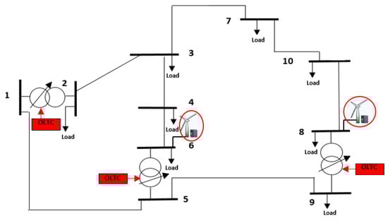
Figure 6.
The topology of the 10-bus test network.
The system has two voltage levels, ultra-high voltage (220 kV) and high voltage (110 kV). Buses 2, 3, 6, 7, 8, and 10 belong to the high voltage level (110 kV), and buses 1, 5, and 9 have an ultra-high voltage level (220 kV). On the other hand, buses 2, 3, 4, 5, 7, and 10 belong to the category of load buses, Buses 6 and 8 are generation buses, and Bus 1 represents the slack-bus. Two wind farms with an installed capacity of 50 MW are connected to Buses 6 and 8 through electric lines with short lengths. The three power transformers (T(1,2), T(5,6), and T(8,9)) have the on-load tap changer (OLTC) so that the possibility to implement the proposed coordinated control methodology is accomplished. The power transformers have the following initial tap positions, tap 15 for T(1,2), tap 10 for T(5,6), and tap 8 for T(8,9), which ensure a high voltage level at the 110 kV buses (between 1.05 and 1.1 pu.). The Supplementary File Network Data contains the technical characteristics of the electric lines and power transformers.
The analysis has been performed considering one day as the study period. The active and reactive power profiles requested by the loads and injected by the two wind farms in the analyzed day have been uploaded from the database of the SCADA master system. The Supplementary File Power Profiles contains the profiles associated with each load bus and Wind Farm.
The obtained results have been compared with a base scenario (S0) where both wind farms are OFF to quantify the benefits on the operation of the network with the wind power sources integrated, overlapping the coordinated control of the OLTCs.
The results for the 220 kV buses are not presented in the case study because the voltage variation is very close during the analyzed period, and the coordinated control OLTCs operate at the level of the 110 kV buses.
Figure 7 presents the hourly values of the objective function (1) obtained in the base scenario S0, without (solid line) and with (square dots and blue bars) coordinated control of the OLTCs in the analyzed network, the power savings are also shown (red bars). The power flow was calculated using the Newton–Raphson method.
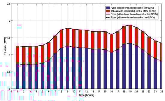
Figure 7.
The hourly values of the objective function (without and with coordinated control of the OLTCs) and the energy-savings, base scenario S0.
Table 5 presents the numerical values of the objective function (1) obtained in the base scenario S0, without (F*Loss,h) and with (F**Loss,h) coordinated control of the OLTCs in the analyzed network, the power saving (ΔFLoss) in absolute and percent units and tap positions resulting from the optimization process.
Table 5.
The results obtained without and with coordinated control of the OLTCs, scenario S0.
The hourly power savings have been calculated with the formula:
where: ΔFLoss,h (MW) is the power saving calculated in MW at hour h; ΔFLoss,h (%) is the power saving calculated in percent at hour h; represents the power losses calculated without a coordinated control of the OLTCs at the hour h; represents the power losses calculated with coordinated control of the OLTCs at the hour h.
The energy-savings have values between 28.34% (recorded at hour 19) and 42.74% (recorded at hour 2), with a mean of 34.13%. The energy-saving in the analyzed period was 12.62 MWh, representing 33.47% of the total energy losses (37.7 MWh) calculated without a coordinated control of the OLTCs.
The energy-saving, ES, in the analyzed period has been calculated with the formula:
Three time intervals resulted in the optimization process of the tap positions, namely: (1–7,8–21), and (22–24). Thus, transformer T(1,2) has the tap changer mainly at position 8 in the first time interval (6 out of 7 h), at position 10 in the second time interval (13 out of 14 h), and at position 9 in the third time interval. The last transformers, T(5,6) and T(8,9), have the same positions of the tap changer most of the time, namely: position 7 in the first interval (7 out of 8 h), position 9 in the second interval (12 out of 14 h), and position 8 in the third interval, see Figure 8. The number of turns for the tap changers of transformers T(1,2) and T(5,6) is 6 and for transformer T(8,9) is 8 in the analyzed period to keep the voltage at the level of each bus within an optimal range corresponding to minimum power losses in the network.
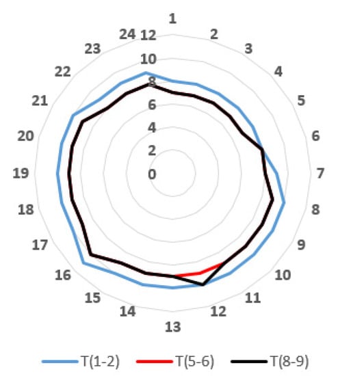
Figure 8.
The radar display of the tap positions resulted from the optimization process.
Figure 9 shows the voltage variation at the 110 kV buses in the base scenario S0, without and with coordinated control of the OLTCs. Table A1 from Appendix A presents the hourly values of the voltage at each bus, without and with coordinated control of the OLTCs.
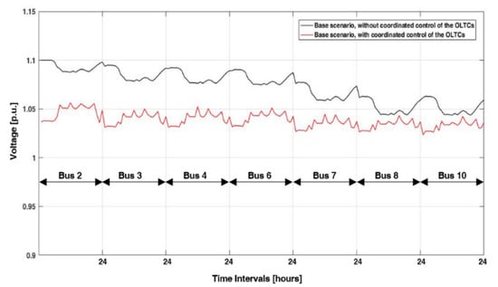
Figure 9.
The variation of the voltage at the 110 kV buses in the analyzed period (24 h), base scenario S0.
A statistical analysis based on a boxplot has been considered to highlight details on the voltage variations in the network. The boxplot includes the most significant statistical features of the voltage, providing a better understanding and comparison for each bus and whole network [43].
The boxplot graphically represents five values of distribution regarding the minimum value, Q0, the first quartile, Q1 (or lower quartile), the median, Q2, the third quartile, Q3 (or upper quartile), and the maximum value, Q4 [44], see Figure 10a. The median voltage at the buses (drawn with a red line inside each box), without coordinated control of the OLTCs, has a significant multi-step decrease identifying four groups: Group 1 (Buses 2), with Q2 = 1.091; Group 2 (Buses 3, 4, and 6) with Q2 between 1.078 and 1.082; Group 3 (Bus 7) with Q2 = 1.063, and Group 4 (Buses 8 and 10) with Q2 = 1.048. The interquartile ranges are reasonably similar for all buses, as seen by the lengths of the boxes represented with the blue color in the figure (lower and upper sides of the box, named quartiles Q1 and Q3). The voltage distribution is positioned towards the upper side of the box for all buses, observable through longer whiskers and larger areas over the median, quartile Q2 (red line from inside the box), see Figure 10a. Regarding the coordinated control of the OLTCs, the median voltage (Q2) at buses is closer, with a reduced difference of about 0.017 between Group 1 (Bus 2, Q2 = 1.051) and Group 4 (Buses 8 and 10, Q2 = 1.034). The interquartile ranges are similar for all buses, as seen by the lengths of the boxes, except Bus 2, which is smaller, see Figure 10b. The voltage distribution is positioned towards the lower side of the box for all buses, observable through longer whiskers and larger areas under the median, quartile Q2. Furthermore, neither bus presents any suspiciously far-out values (outliers) of the voltage that might require a deeper analysis.
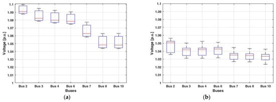
Figure 10.
The boxplot of the voltage at the level of the 110 kV buses, scenario S0: (a) without coordinated control of the OLTCs; (b) with coordinated control of the OLTCs.
Table 6 shows the statistical details with the calculated values of the quartiles. These statistical indicators confirm reaching the objective, regarded as constant as possible voltage level in the electric network, in an optimal variation range, such that the power losses have the lowest values if the proposed coordinated control methodology is applied.
Table 6.
The statistical parameters associated with the voltage at the buses, scenario S0.
In the following, the scenario with the integration of the wind farms in the network (named S1) has been analyzed. Three cases have been considered to investigate the optimal operation of the network.
- Case 1: Wind Farm 1 (connected at the bus 6) is ON, and Wind Farm 2 (connected at the bus 8) is OFF;
- Case 2: Wind Farm 1 (connected at the bus 6) is OFF, and Wind Farm 2 (connected at the bus 8) is ON;
- Case 3: Both wind farms are ON.
The obtained results are compared with the base scenario S0, when both wind farms were OFF, to quantify the benefits on the operation of the network with the wind power sources integrated, overlapping the coordinated control of the OLTCs. The details of the analysis for each case are presented in the following.
Figure 11 presents the hourly values of the objective function (1), without (solid line) and with (square dots and blue bars) coordinated control of the OLTCs in the analyzed network, and the power savings (red bars) in the three analyzed cases. The power flow was calculated using the Newton–Raphson method.

Figure 11.
The hourly values of the objective function (without and with coordinated control of the OLTCs) and the energy-savings, in the three cases of scenario S1: (a) Case 1; (b) Case 2; (c) Case 3.
Table 7 presents the numerical values of the objective function (1), without (F*Loss) and with (F**Loss) coordinated control of the OLTCs in the analyzed network, the power savings (ΔFLoss) in absolute and percent units, and tap positions resulting from the optimization process in the three analyzed cases. The hourly power saving corresponding to each case has been calculated via Formula (31). The energy-savings in the three cases exceed 30%, having the minimum values recorded at hour 19 (31.33%, Case 1, 31.54%, Case 2, and 35.34%, Case 3) and the maximum values recorded at hour 2 (45.79%, Case 1, 46,67%, Case 2, and 50%, Case 3). The means in the three cases are 37.51%, 37.92%, and 41.58%, respectively. The total energy-savings in the analyzed period are 36.82%, 37.42%, and 41.27% of the total energy losses (30.88, 30.30, and 24.52 MWh, respectively) recorded when the coordinated control of the OLTCs is not used.
Table 7.
The results obtained without and with coordinated control of the OLTCs, scenario S1.
Figure 12 presents the tap positions of each transformer depending on the analyzed case. Thus, the transformers have the changers at different taps in the three time intervals ((1–7,8–21), and (22–24)) and analyzed cases. Transformer T(1,2) has the tap changer at positions (8–10) in the first time interval, (9–12) in the second time interval, and (8,9) in the third time interval. Transformer T(5,6) has the tap changer at positions (6–8) in the first interval, (8–10) in the second time interval, and (7,8) in the third time interval. The transformer T(8,9) has the tap changer at the same positions, (7–9) in the first and third intervals, and (7–10) in the second time interval.
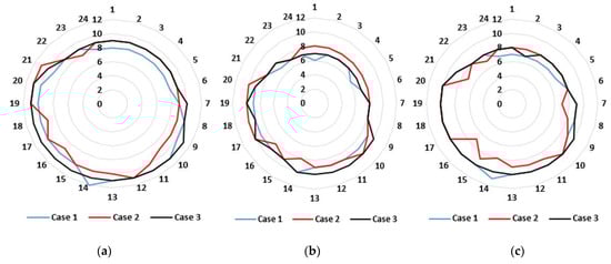
Figure 12.
The radar display of the tap positions resulted from the optimization process associated with scenario S1: (a) transformer T(1,2); (b) transformer T(5,6); (c) transformer T(8,9).
However, the number of turns for the tap changers is different for the three transformers in the analyzed cases to keep the voltage at the level of each bus within an optimal range corresponding to minimum power losses in the network, see Figure 13.
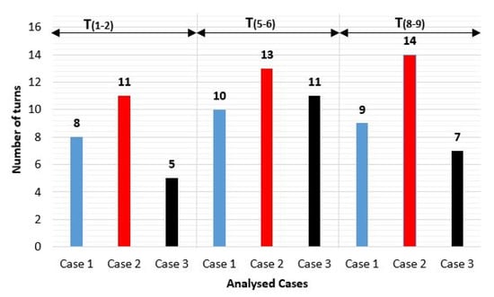
Figure 13.
The number of turns for the tap changers of the three transformers in the three analyzed cases of scenario S1.
A high number of turns is recorded in Case 2 (14 turns recorded for the transformer T(8,9)) followed by Case 1 (10 turns recorded for transformer T(5,6)) and Case 3 (11 turns recorded for transformer T(5,6)). The number is higher in Cases 1 and 2 for all transformers than in scenario S0, where six turns are performed by transformers T(1,2) and T(5,6) and eight for transformer T(8,9). Fewer turns are recorded in Case 3 for transformers T(1,2) and T(8,9) (five and seven, respectively) and almost double-figure turns for transformer T(5,6) to ensure a voltage level was in a narrow range.
Figure 14 shows the voltage variation at the 110 kV buses, without and with coordinated control of the OLTCs. Table A2, Table A3 and Table A4 from Appendix A present the hourly values of the voltage at each bus, without and with coordinated control of the OLTCs, in the three analyzed cases. The voltage at the buses has a variation between 1.1 (Bus 2) and 1.05 (Bus 10, Case 1). The highest values are recorded in the time intervals (1–7) and (22–24). The variation is reduced at 0.03 p.u., being very close at each bus, if the coordinated control of OLTCs is used. The exploratory analysis based on the voltage boxplots confirmed this statement.
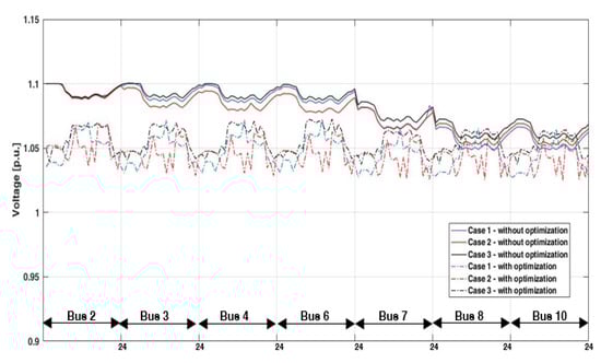
Figure 14.
The variation of the voltage at the 110 kV buses in the analyzed period (24 h) in the three analyzed cases of scenario S1.
Figure 15 shows that the median voltage at the buses (drawn with a red line inside each box), when the coordinated control of the OLTCs is not used, and it has a multi-step decrease slightly attenuated for the four groups in the three analyzed cases compared to in scenario S0: Group 1 (Buses 2) between Q2 = 1.091 and 1.092, Group 2 (Buses 3, 4, and 6) with Q2 between 1.081 and 1.092, Group 3 (Bus 7) with Q2 between 1.068 and 1.074, and Group 4 (Buses 8 and 10) with Q2 between 1.053 and 1.061.
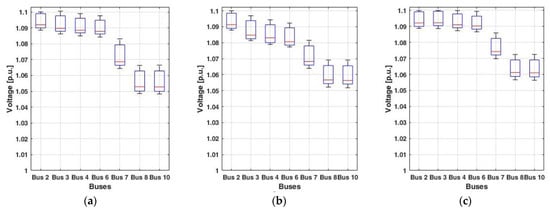
Figure 15.
The boxplots of the voltage at the level of the 110 kV buses, scenario S1—without coordinated control of the OLTCs: (a) Case 1; (b) Case 2; (c) Case 3.
This decrease is attenuated between groups from Case 1 to Case 3 (see Table 8, Table 9 and Table 10). At the same time, the median voltage from Groups 3 and 4 in Case 3 increases to 1.074 and 1.061, respectively. The interquartile ranges are reasonably similar in all cases, as seen by the lengths of the boxes (lower and upper sides of the box). The voltage distribution at all buses is positively skewed in all cases, being observable, the whisker and half-box are longer on the lower side of the median than on the upper side. Buses 2 and 6 present a few outliers of the voltage but, these values are very close to the quintile Q4, without being considered a problem.
Table 8.
The statistical parameters associated with the voltage at the buses, scenario S1, Case 1.
Table 9.
The statistical parameters associated with the voltage at the buses, scenario S1, Case 2.
Table 10.
The statistical parameters associated with the voltage at the buses, scenario S1, Case 3.
The obtained data are different when the coordinated control of the OLTCs is used, as can be seen in Figure 16.
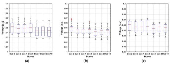
Figure 16.
The boxplots of the voltage at the level of the 110 kV buses, scenario S1—with coordinated control of the OLTCs: (a) Case 1; (b) Case 2; (c) Case 3.
The median voltage at the buses is close, with reduced differences of about 0.01. The interquartile ranges have similar sizes for all buses in the first two cases and are slightly different in Case 3 for the four groups. The distributions in Cases 1 and 3 are approximately symmetric because both half-boxes are almost the same length. Regarding Case 2, the voltage distribution at all buses is negatively skewed, being observable, the whisker and half-box are longer on the lower side of the median than on the upper side, see Table 8, Table 9 and Table 10.
The simulations run on a computer with an Intel Core i7 processor, 3.4 GHz, and 8 GB RAM, and the source code has been written in Matlab.
The authors highlighted, in Paragraph 1.1, higher performances of classical algorithms from the mathematical programming compared to the meta-heuristic algorithms. Thus, one of the most efficient classical methods, the reduced gradient method (RG-CC), [32,33], was chosen to compare the results and demonstrate the efficiency of the proposed method considering the average computational time (CTav) and the value of the objective function, FLoss, in the three cases, see Table 11.
where cth,c refers to the computing time in which the solution of the OPF problem was obtained for hour h, h = 1, …, TH, and the case c, c = 1, …, Ncases.
Table 11.
Comparison between the computational times.
It can be observed that the time computational, CTav, is 31% faster than in the RG-CC, which demonstrates that the SQP-CC can be successfully implemented in real-time to change the tap positions. The second indicator highlights the accuracy of the SQP-CC methodology. In all three analyzed cases, FLoss associated with the SQP-CC is smaller than in the RG-CC, by 1.32%, 3.07%, and 2.64%, respectively.
4. Conclusions
The paper addressed the OPF problem in the electric networks integrating wind farms. The main objective aimed to determine an as constant as possible voltage level at each bus, if possible, in a variation interval as narrow as possible, such that the power losses have the lowest value. An SQP-CC methodology of the OLTCs was proposed, such that the optimal voltage level at the buses led to the minimum active power losses. Their practical implementation has, as the starting point, the ability of the TSOs to hold the control capability of the transformers with OLTC due to the advanced technologies based on the automatic voltage control (AVC). It can work in both operation modes (real-time and off-line). The methodology works in real-time with input data collected from the SCADA system at different periods by sampling steps (1, 5, 10, 15, 30, or 60 min). Using the same sampling steps, having the lowest possible value for all RTUs, represents a solution adopted at the level of the SCADA system, which includes the frequent changes in the wind generation.
The effectiveness of the proposed SQP-CC methodology was tested on a 10-bus network, representing a zone of a real transmission and distribution system, with two wind farms connected. Two scenarios were analyzed, without and with wind farms connected, to quantify the benefits on the operation of the network with the wind power sources integrated overlapping the coordinated control of the OLTCs. Three specific cases were considered in the second scenario: Case 1: Wind Farm 1 is ON, Wind Farm 2 is OFF; Case 2: Wind Farm 1 is OFF, Wind Farm 2 is ON; Case 3: both wind farms are ON. The energy-saving, calculated by formula (32), was 33.5% in the scenario without wind farms connected and applying the SQP-CC methodology. Higher values were obtained in the three cases of the second scenario, 36.8% (Case 1), 37.42% (Case 2), and 41.27% (Case 3). The optimal tap positions of the transformers led to the very close voltage variations between the 110 kV buses of the network compared to not using the SQP-CC methodology. The average voltage drop between Bus 2 and Bus 10 in the three cases was by 0.008, 0.009, and 0.004 p.u., respectively, compared to 0.038, 0.034, and 0.031 p.u., without the SQP-CC methodology.
From the point of view of DNOs and TSOs, the considered scenarios, without and with wind farms connected (together with the three cases analyzed within the second scenario), cover all of the situations associated with the steady-state of the electrical networks. Of course, the results will be different when new wind farms are connected, but the benefits on the operation of the network with the wind power sources integrated overlapping the coordinated control of the OLTCs will always be positive.
The performance associated with the average time computing obtained in the analyzed cases was better compared with the RG-CC (0.24 versus 0.35 s). All results emphasized the effectiveness of the proposed control methodology.
The implementation of the proposed methodology can be limited by the following technical features: the OPF module integrated into the software has a fast processing speed, the wide-area communication network has a high-speed data transmission, and the OLTC of the transformer performs quick changing of the taps.
The authors now work with an improved variant of the OPF model, which considers a new constraint regarding minimum turns of the tap to avoid the overuse of the contact wear of the OLTC. Moreover, the influence of the changes in the wind generation, which can occur within the time interval associated with the sampling step, and the missing data due to a technical failure at the communication network of the SCADA system, represent another future work to evaluate the impact on the obtained solutions. These aspects will be tested using an extension of the test network, from the considered zone of the transmission and distribution system containing more buses, and will be analyzed to verify the effectiveness of the SQP-CC methodology based on the improved OPF model.
Supplementary Materials
The following supporting information can be downloaded at https://www.mdpi.com/article/10.3390/app12031129/s1. File Network Data. xlsx; File Power Profiles. xlsx.
Author Contributions
Conceptualization, G.G.; methodology, G.G., B.-C.N. and O.I.; software, G.G.; validation, B.L., B.-C.N., F.S. and O.I.; formal analysis, B.-C.N., O.I., B.L. and F.S.; investigation, G.G., B.-C.N., F.S., B.L. and O.I.; writing—original draft preparation, G.G., B.-C.N., F.S. and O.I.; writing—review and editing, G.G., O.I. and B.-C.N.; and supervision, G.G. All authors have read and agreed to the published version of the manuscript.
Funding
This research received no external funding.
Institutional Review Board Statement
Not applicable.
Informed Consent Statement
Not applicable.
Conflicts of Interest
The authors declare no conflict of interest.
Nomenclature and Indices
| OPF | Optimal power flow |
| DNO | Distribution Network Operator |
| TSO | Transmission System Operator |
| SQP | Successive quadratic programming |
| RG | Reduced Gradient |
| CC | Centralized control |
| SCADA | Supervisory Control and Data Acquisition |
| EU | European Union |
| NECP | National Energy and Climate Plan |
| DM | Decision-Maker |
| OLTC | On-load tap changers |
| RTU | Remote terminal unit |
| CDC | Central data concentrator |
| AVC | Automatic voltage control |
| IEEE | Institute of Electrical and Electronics Engineers |
| DC | Direct Current |
| VA | structure vector recording records areas of the electric network |
| VE | structure vector containing elements (electric line/power transformer from each area recorded in the vector VA |
| SB | slack bus |
| Nw | the set of wind generator buses in the network |
| N | the set of all buses in the network |
| E | the total number of the elements (lines and transformers) in the networks |
| s | index for the slack bus |
| Ng | the set of conventional generator buses in the network |
| Ge | the real part of element e between the i-th bus and j-th bus from the nodal admittance matrix |
| TH | the analyzed time period |
| Vi,h | the voltage magnitude at the i-th bus and hour h, in (kV) |
| Vj,h | the voltage magnitude at the j-th bus and hour h, in (kV) |
| Gij | the real part of element ij from nodal admittance matrix |
| Bij | the imaginary part of element ij from nodal admittance matrix |
| PGi,h, QGi,h | the active and reactive powers generated at the i-th bus and hour h, in (MW) and (MVAr) |
| PLi,h, QLi,h | the active and reactive powers required at the i-th bus and hour h, in (MW) and (MVAr) |
| tij,h | the tap position of the transformer connected between the i-th bus and j-th bus and hour h |
| Sij max | the maximum load of the line connected between the i-th bus and j-th bus, in (MVA) |
| PGlmin, PGlmax | the active power limits of the l-th conventional power plant, in (MW) |
| QGlmin, QGlmax | the reactive power limits of the l-th conventional power plant, in (MVAr) |
| Pwmin, Pwmax | the active power limits of the w-th wind farm, in (MW) |
| Pw | the active power of the w-th wind farm, in (MW) |
| [X] | the optimization vector |
| F([X]) | objective function |
| hAi([X]) | the equality restriction i, i = 1, …, p |
| p | the number of the active equality restrictions |
| hIj([X]) | the inactive inequality restriction j, j = 1, …, q |
| q | the number of the equality restrictions |
| [X(0)] | a feasible starting point of the optimization process |
| Z([ΔX]) | the objective function of the QP problem |
| [ΔX] | the vector of the optimization variables associated with the QP problem |
| [H] | the Hessian of the objective function |
| F(0) | the value of the objective function F calculated at the starting point [X(0)] |
| the gradient of the objective function calculated at the starting point [X(0)] | |
| [hA(0)] | the vector of the active constraints at the starting point [X(0)] |
| [hI(0)] | the vector of the inactive constraints at the starting point [X(0)] |
| [JA] | the Jacobian of the active constraints |
| [JI] | the Jacobian of the inactive constraints |
| [∆Z] | the control (independent) variables |
| [∆Y] | the state (dependent) variables |
| αopt(k) | the optimal value of step size |
| αadm(k) | the admissible value of the step size |
| ΔFLoss,h(MW) | the power saving calculated in MW at hour h |
| ΔFLoss,h (%) | the power saving calculated in percent at hour h |
| F*Loss,h | the power losses calculated without a coordinated control of the OLTCs at the hour h, in (MW) |
| F**Loss,h | the power losses calculated with coordinated control of the OLTCs at the hour h, in (MW) |
| ES(MWh) | the energy-saving calculated in MWh |
| ES(%) | the energy-saving calculated in percent |
| Q0–Q4 | the quartiles |
| CTav | the average computational time |
| cth,c | the computing time in which the solution of the OPF problem was obtained for hour h, h = 1, …, TH, and the case c, c = 1, …, Ncases. |
| Ncases | the number of analyzed cases |
Appendix A
Table A1.
The hourly values of the voltage at each bus, scenario S0.
Table A1.
The hourly values of the voltage at each bus, scenario S0.
| Hour | without Coordinated Control of the OLTCs | with Coordinated Control of the OLTCs | ||||||||||||
|---|---|---|---|---|---|---|---|---|---|---|---|---|---|---|
| Bus2 | Bus3 | Bus4 | Bus6 | Bus7 | Bus8 | Bus10 | Bus2 | Bus3 | Bus4 | Bus6 | Bus7 | Bus8 | Bus10 | |
| 1 | 1.100 | 1.094 | 1.091 | 1.089 | 1.076 | 1.062 | 1.062 | 1.037 | 1.031 | 1.031 | 1.032 | 1.027 | 1.027 | 1.023 |
| 2 | 1.100 | 1.095 | 1.092 | 1.090 | 1.077 | 1.063 | 1.063 | 1.038 | 1.032 | 1.032 | 1.033 | 1.028 | 1.028 | 1.027 |
| 3 | 1.100 | 1.095 | 1.092 | 1.090 | 1.077 | 1.063 | 1.063 | 1.038 | 1.032 | 1.032 | 1.033 | 1.028 | 1.028 | 1.027 |
| 4 | 1.100 | 1.095 | 1.092 | 1.090 | 1.077 | 1.063 | 1.063 | 1.038 | 1.032 | 1.032 | 1.033 | 1.028 | 1.028 | 1.027 |
| 5 | 1.100 | 1.094 | 1.092 | 1.090 | 1.076 | 1.062 | 1.062 | 1.037 | 1.031 | 1.031 | 1.032 | 1.027 | 1.027 | 1.026 |
| 6 | 1.098 | 1.092 | 1.089 | 1.088 | 1.074 | 1.059 | 1.059 | 1.038 | 1.037 | 1.037 | 1.039 | 1.033 | 1.034 | 1.033 |
| 7 | 1.093 | 1.085 | 1.083 | 1.081 | 1.066 | 1.051 | 1.051 | 1.042 | 1.035 | 1.035 | 1.036 | 1.029 | 1.029 | 1.028 |
| 8 | 1.091 | 1.082 | 1.080 | 1.078 | 1.063 | 1.048 | 1.048 | 1.054 | 1.046 | 1.046 | 1.047 | 1.039 | 1.038 | 1.038 |
| 9 | 1.088 | 1.079 | 1.077 | 1.075 | 1.059 | 1.044 | 1.044 | 1.051 | 1.042 | 1.042 | 1.043 | 1.035 | 1.034 | 1.034 |
| 10 | 1.088 | 1.079 | 1.077 | 1.075 | 1.059 | 1.045 | 1.044 | 1.051 | 1.042 | 1.042 | 1.043 | 1.035 | 1.035 | 1.034 |
| 11 | 1.088 | 1.079 | 1.077 | 1.075 | 1.059 | 1.044 | 1.044 | 1.051 | 1.042 | 1.042 | 1.043 | 1.035 | 1.034 | 1.034 |
| 12 | 1.088 | 1.078 | 1.076 | 1.075 | 1.059 | 1.044 | 1.044 | 1.056 | 1.049 | 1.052 | 1.048 | 1.045 | 1.037 | 1.036 |
| 13 | 1.089 | 1.080 | 1.078 | 1.076 | 1.060 | 1.046 | 1.045 | 1.051 | 1.043 | 1.043 | 1.044 | 1.036 | 1.036 | 1.035 |
| 14 | 1.088 | 1.079 | 1.076 | 1.075 | 1.059 | 1.044 | 1.044 | 1.050 | 1.041 | 1.041 | 1.043 | 1.035 | 1.034 | 1.033 |
| 15 | 1.089 | 1.081 | 1.078 | 1.077 | 1.061 | 1.046 | 1.046 | 1.052 | 1.044 | 1.044 | 1.045 | 1.037 | 1.037 | 1.036 |
| 16 | 1.091 | 1.082 | 1.080 | 1.078 | 1.063 | 1.049 | 1.048 | 1.055 | 1.050 | 1.050 | 1.051 | 1.044 | 1.043 | 1.043 |
| 17 | 1.090 | 1.082 | 1.079 | 1.078 | 1.062 | 1.048 | 1.047 | 1.053 | 1.045 | 1.045 | 1.046 | 1.038 | 1.038 | 1.037 |
| 18 | 1.089 | 1.080 | 1.077 | 1.076 | 1.060 | 1.045 | 1.045 | 1.052 | 1.043 | 1.043 | 1.044 | 1.036 | 1.035 | 1.034 |
| 19 | 1.088 | 1.079 | 1.076 | 1.075 | 1.058 | 1.044 | 1.044 | 1.051 | 1.041 | 1.042 | 1.043 | 1.034 | 1.034 | 1.033 |
| 20 | 1.090 | 1.081 | 1.079 | 1.077 | 1.061 | 1.047 | 1.046 | 1.053 | 1.044 | 1.044 | 1.045 | 1.037 | 1.037 | 1.036 |
| 21 | 1.092 | 1.084 | 1.081 | 1.080 | 1.064 | 1.050 | 1.050 | 1.056 | 1.047 | 1.047 | 1.048 | 1.041 | 1.040 | 1.040 |
| 22 | 1.095 | 1.087 | 1.085 | 1.083 | 1.068 | 1.054 | 1.054 | 1.044 | 1.037 | 1.037 | 1.038 | 1.031 | 1.031 | 1.030 |
| 23 | 1.097 | 1.090 | 1.087 | 1.085 | 1.071 | 1.057 | 1.057 | 1.036 | 1.034 | 1.035 | 1.036 | 1.031 | 1.031 | 1.031 |
| 24 | 1.098 | 1.092 | 1.089 | 1.087 | 1.074 | 1.059 | 1.059 | 1.049 | 1.042 | 1.042 | 1.043 | 1.037 | 1.037 | 1.036 |
Table A2.
The hourly values of the voltage at each bus, Case 1, scenario S1.
Table A2.
The hourly values of the voltage at each bus, Case 1, scenario S1.
| Hour | without Coordinated Control of the OLTCs | with Coordinated Control of the OLTCs | ||||||||||||
|---|---|---|---|---|---|---|---|---|---|---|---|---|---|---|
| Bus2 | Bus3 | Bus4 | Bus6 | Bus7 | Bus8 | Bus10 | Bus2 | Bus3 | Bus4 | Bus6 | Bus7 | Bus8 | Bus10 | |
| 1 | 1.100 | 1.099 | 1.097 | 1.095 | 1.080 | 1.065 | 1.065 | 1.035 | 1.031 | 1.031 | 1.031 | 1.028 | 1.028 | 1.028 |
| 2 | 1.100 | 1.101 | 1.099 | 1.098 | 1.082 | 1.066 | 1.066 | 1.039 | 1.039 | 1.040 | 1.041 | 1.033 | 1.031 | 1.031 |
| 3 | 1.100 | 1.100 | 1.099 | 1.098 | 1.082 | 1.066 | 1.066 | 1.039 | 1.038 | 1.039 | 1.041 | 1.033 | 1.031 | 1.031 |
| 4 | 1.100 | 1.100 | 1.099 | 1.097 | 1.082 | 1.066 | 1.066 | 1.039 | 1.038 | 1.039 | 1.040 | 1.033 | 1.031 | 1.031 |
| 5 | 1.100 | 1.099 | 1.098 | 1.096 | 1.081 | 1.065 | 1.065 | 1.036 | 1.032 | 1.032 | 1.032 | 1.028 | 1.029 | 1.028 |
| 6 | 1.099 | 1.098 | 1.097 | 1.095 | 1.079 | 1.063 | 1.063 | 1.037 | 1.038 | 1.038 | 1.039 | 1.035 | 1.037 | 1.036 |
| 7 | 1.094 | 1.092 | 1.090 | 1.089 | 1.071 | 1.056 | 1.055 | 1.044 | 1.044 | 1.044 | 1.046 | 1.040 | 1.042 | 1.041 |
| 8 | 1.092 | 1.089 | 1.087 | 1.086 | 1.068 | 1.052 | 1.052 | 1.053 | 1.046 | 1.046 | 1.047 | 1.041 | 1.041 | 1.040 |
| 9 | 1.089 | 1.087 | 1.086 | 1.085 | 1.065 | 1.049 | 1.049 | 1.065 | 1.058 | 1.058 | 1.059 | 1.052 | 1.052 | 1.051 |
| 10 | 1.090 | 1.088 | 1.088 | 1.087 | 1.067 | 1.050 | 1.050 | 1.065 | 1.060 | 1.060 | 1.061 | 1.053 | 1.053 | 1.052 |
| 11 | 1.089 | 1.088 | 1.087 | 1.086 | 1.066 | 1.050 | 1.050 | 1.065 | 1.059 | 1.059 | 1.060 | 1.053 | 1.053 | 1.052 |
| 12 | 1.089 | 1.086 | 1.085 | 1.085 | 1.065 | 1.049 | 1.049 | 1.064 | 1.058 | 1.058 | 1.059 | 1.052 | 1.052 | 1.051 |
| 13 | 1.090 | 1.088 | 1.087 | 1.086 | 1.067 | 1.051 | 1.050 | 1.065 | 1.059 | 1.060 | 1.060 | 1.053 | 1.053 | 1.053 |
| 14 | 1.089 | 1.086 | 1.085 | 1.085 | 1.065 | 1.049 | 1.049 | 1.070 | 1.072 | 1.072 | 1.072 | 1.066 | 1.066 | 1.065 |
| 15 | 1.090 | 1.088 | 1.087 | 1.086 | 1.067 | 1.051 | 1.051 | 1.054 | 1.053 | 1.054 | 1.055 | 1.049 | 1.050 | 1.050 |
| 16 | 1.092 | 1.090 | 1.089 | 1.088 | 1.069 | 1.053 | 1.053 | 1.056 | 1.055 | 1.056 | 1.057 | 1.051 | 1.053 | 1.052 |
| 17 | 1.091 | 1.090 | 1.088 | 1.088 | 1.068 | 1.052 | 1.052 | 1.055 | 1.055 | 1.056 | 1.057 | 1.051 | 1.052 | 1.051 |
| 18 | 1.090 | 1.087 | 1.086 | 1.085 | 1.066 | 1.050 | 1.049 | 1.054 | 1.052 | 1.053 | 1.055 | 1.048 | 1.049 | 1.048 |
| 19 | 1.091 | 1.086 | 1.085 | 1.084 | 1.064 | 1.049 | 1.048 | 1.053 | 1.051 | 1.052 | 1.053 | 1.046 | 1.048 | 1.047 |
| 20 | 1.091 | 1.089 | 1.087 | 1.086 | 1.067 | 1.051 | 1.051 | 1.055 | 1.054 | 1.055 | 1.056 | 1.049 | 1.051 | 1.050 |
| 21 | 1.093 | 1.091 | 1.090 | 1.089 | 1.070 | 1.054 | 1.054 | 1.043 | 1.043 | 1.044 | 1.045 | 1.039 | 1.041 | 1.040 |
| 22 | 1.096 | 1.094 | 1.092 | 1.091 | 1.073 | 1.058 | 1.058 | 1.043 | 1.038 | 1.038 | 1.039 | 1.034 | 1.034 | 1.033 |
| 23 | 1.097 | 1.095 | 1.093 | 1.092 | 1.083 | 1.060 | 1.060 | 1.045 | 1.040 | 1.040 | 1.040 | 1.036 | 1.037 | 1.036 |
| 24 | 1.099 | 1.097 | 1.096 | 1.094 | 1.078 | 1.063 | 1.063 | 1.036 | 1.035 | 1.036 | 1.037 | 1.029 | 1.027 | 1.027 |
Table A3.
The hourly values of the voltage at each bus, Case 2, scenario S1.
Table A3.
The hourly values of the voltage at each bus, Case 2, scenario S1.
| Hour | without Coordinated Control of the OLTCs | with Coordinated Control of the OLTCs | ||||||||||||
|---|---|---|---|---|---|---|---|---|---|---|---|---|---|---|
| Bus2 | Bus3 | Bus4 | Bus6 | Bus7 | Bus8 | Bus10 | Bus2 | Bus3 | Bus4 | Bus6 | Bus7 | Bus8 | Bus10 | |
| 1 | 1.100 | 1.095 | 1.093 | 1.091 | 1.080 | 1.067 | 1.067 | 1.051 | 1.046 | 1.046 | 1.046 | 1.044 | 1.045 | 1.044 |
| 2 | 1.100 | 1.097 | 1.094 | 1.092 | 1.082 | 1.069 | 1.069 | 1.052 | 1.048 | 1.048 | 1.048 | 1.046 | 1.047 | 1.047 |
| 3 | 1.100 | 1.097 | 1.094 | 1.092 | 1.081 | 1.069 | 1.069 | 1.052 | 1.047 | 1.047 | 1.048 | 1.045 | 1.047 | 1.046 |
| 4 | 1.100 | 1.097 | 1.094 | 1.092 | 1.081 | 1.069 | 1.069 | 1.052 | 1.047 | 1.047 | 1.048 | 1.045 | 1.047 | 1.045 |
| 5 | 1.100 | 1.096 | 1.093 | 1.091 | 1.080 | 1.068 | 1.068 | 1.051 | 1.047 | 1.047 | 1.047 | 1.044 | 1.046 | 1.045 |
| 6 | 1.099 | 1.094 | 1.092 | 1.090 | 1.078 | 1.066 | 1.066 | 1.049 | 1.045 | 1.044 | 1.045 | 1.042 | 1.044 | 1.043 |
| 7 | 1.093 | 1.087 | 1.085 | 1.083 | 1.071 | 1.059 | 1.059 | 1.042 | 1.035 | 1.036 | 1.037 | 1.029 | 1.028 | 1.027 |
| 8 | 1.092 | 1.085 | 1.082 | 1.081 | 1.067 | 1.055 | 1.055 | 1.040 | 1.034 | 1.034 | 1.035 | 1.030 | 1.032 | 1.031 |
| 9 | 1.089 | 1.082 | 1.079 | 1.078 | 1.065 | 1.053 | 1.053 | 1.051 | 1.045 | 1.045 | 1.046 | 1.041 | 1.043 | 1.042 |
| 10 | 1.089 | 1.083 | 1.080 | 1.079 | 1.066 | 1.055 | 1.055 | 1.066 | 1.060 | 1.060 | 1.060 | 1.056 | 1.059 | 1.058 |
| 11 | 1.089 | 1.082 | 1.080 | 1.078 | 1.066 | 1.054 | 1.054 | 1.051 | 1.045 | 1.045 | 1.046 | 1.042 | 1.044 | 1.044 |
| 12 | 1.088 | 1.081 | 1.079 | 1.077 | 1.065 | 1.053 | 1.053 | 1.050 | 1.044 | 1.044 | 1.045 | 1.041 | 1.043 | 1.042 |
| 13 | 1.089 | 1.083 | 1.080 | 1.079 | 1.066 | 1.055 | 1.054 | 1.052 | 1.046 | 1.046 | 1.047 | 1.043 | 1.045 | 1.044 |
| 14 | 1.088 | 1.081 | 1.079 | 1.078 | 1.065 | 1.053 | 1.053 | 1.036 | 1.030 | 1.030 | 1.032 | 1.027 | 1.030 | 1.029 |
| 15 | 1.090 | 1.083 | 1.081 | 1.079 | 1.067 | 1.055 | 1.054 | 1.053 | 1.046 | 1.046 | 1.047 | 1.043 | 1.045 | 1.044 |
| 16 | 1.091 | 1.085 | 1.085 | 1.081 | 1.069 | 1.057 | 1.057 | 1.039 | 1.032 | 1.033 | 1.034 | 1.026 | 1.026 | 1.025 |
| 17 | 1.091 | 1.085 | 1.082 | 1.080 | 1.068 | 1.056 | 1.056 | 1.069 | 1.062 | 1.062 | 1.062 | 1.058 | 1.060 | 1.059 |
| 18 | 1.089 | 1.082 | 1.080 | 1.078 | 1.065 | 1.053 | 1.053 | 1.067 | 1.060 | 1.059 | 1.060 | 1.055 | 1.057 | 1.056 |
| 19 | 1.089 | 1.081 | 1.079 | 1.077 | 1.064 | 1.052 | 1.052 | 1.066 | 1.058 | 1.058 | 1.059 | 1.054 | 1.056 | 1.055 |
| 20 | 1.090 | 1.084 | 1.081 | 1.080 | 1.067 | 1.055 | 1.055 | 1.068 | 1.061 | 1.061 | 1.062 | 1.057 | 1.059 | 1.058 |
| 21 | 1.093 | 1.087 | 1.084 | 1.082 | 1.070 | 1.058 | 1.058 | 1.041 | 1.034 | 1.035 | 1.036 | 1.028 | 1.027 | 1.026 |
| 22 | 1.095 | 1.089 | 1.087 | 1.085 | 1.073 | 1.061 | 1.061 | 1.045 | 1.039 | 1.039 | 1.040 | 1.036 | 1.039 | 1.038 |
| 23 | 1.097 | 1.092 | 1.089 | 1.087 | 1.075 | 1.063 | 1.063 | 1.033 | 1.029 | 1.029 | 1.029 | 1.026 | 1.028 | 1.027 |
| 24 | 1.098 | 1.094 | 1.091 | 1.089 | 1.078 | 1.065 | 1.065 | 1.049 | 1.044 | 1.044 | 1.044 | 1.041 | 1.043 | 1.042 |
Table A4.
The hourly values of the voltage at each bus, Case 3, scenario S1.
Table A4.
The hourly values of the voltage at each bus, Case 3, scenario S1.
| Hour | without Coordinated Control of the OLTCs | with Coordinated Control of the OLTCs | ||||||||||||
|---|---|---|---|---|---|---|---|---|---|---|---|---|---|---|
| Bus2 | Bus3 | Bus4 | Bus6 | Bus7 | Bus8 | Bus10 | Bus2 | Bus3 | Bus4 | Bus6 | Bus7 | Bus8 | Bus10 | |
| 1 | 1.100 | 1.100 | 1.098 | 1.097 | 1.083 | 1.070 | 1.070 | 1.049 | 1.047 | 1.045 | 1.045 | 1.044 | 1.047 | 1.046 |
| 2 | 1.100 | 1.100 | 1.100 | 1.099 | 1.086 | 1.073 | 1.073 | 1.039 | 1.045 | 1.041 | 1.043 | 1.037 | 1.038 | 1.037 |
| 3 | 1.100 | 1.100 | 1.100 | 1.099 | 1.086 | 1.072 | 1.072 | 1.051 | 1.040 | 1.048 | 1.048 | 1.047 | 1.049 | 1.049 |
| 4 | 1.100 | 1.100 | 1.100 | 1.099 | 1.086 | 1.072 | 1.072 | 1.051 | 1.048 | 1.047 | 1.048 | 1.047 | 1.049 | 1.049 |
| 5 | 1.100 | 1.100 | 1.099 | 1.098 | 1.084 | 1.071 | 1.071 | 1.050 | 1.048 | 1.046 | 1.046 | 1.045 | 1.048 | 1.047 |
| 6 | 1.099 | 1.100 | 1.099 | 1.097 | 1.083 | 1.070 | 1.070 | 1.048 | 1.046 | 1.045 | 1.046 | 1.044 | 1.047 | 1.046 |
| 7 | 1.094 | 1.094 | 1.093 | 1.092 | 1.076 | 1.063 | 1.063 | 1.056 | 1.045 | 1.052 | 1.052 | 1.050 | 1.052 | 1.052 |
| 8 | 1.092 | 1.091 | 1.089 | 1.088 | 1.072 | 1.059 | 1.058 | 1.054 | 1.052 | 1.048 | 1.049 | 1.045 | 1.048 | 1.047 |
| 9 | 1.090 | 1.090 | 1.088 | 1.088 | 1.071 | 1.058 | 1.058 | 1.067 | 1.048 | 1.068 | 1.070 | 1.061 | 1.062 | 1.061 |
| 10 | 1.090 | 1.091 | 1.091 | 1.090 | 1.073 | 1.060 | 1.060 | 1.068 | 1.067 | 1.070 | 1.072 | 1.064 | 1.064 | 1.063 |
| 11 | 1.090 | 1.091 | 1.090 | 1.089 | 1.073 | 1.060 | 1.059 | 1.067 | 1.069 | 1.069 | 1.071 | 1.063 | 1.063 | 1.062 |
| 12 | 1.089 | 1.089 | 1.088 | 1.087 | 1.071 | 1.058 | 1.057 | 1.066 | 1.068 | 1.068 | 1.069 | 1.061 | 1.061 | 1.061 |
| 13 | 1.090 | 1.091 | 1.090 | 1.089 | 1.073 | 1.059 | 1.059 | 1.068 | 1.066 | 1.069 | 1.071 | 1.063 | 1.063 | 1.062 |
| 14 | 1.089 | 1.089 | 1.088 | 1.087 | 1.071 | 1.057 | 1.057 | 1.066 | 1.068 | 1.067 | 1.069 | 1.061 | 1.061 | 1.060 |
| 15 | 1.091 | 1.090 | 1.089 | 1.088 | 1.072 | 1.059 | 1.059 | 1.066 | 1.066 | 1.062 | 1.062 | 1.059 | 1.062 | 1.061 |
| 16 | 1.092 | 1.092 | 1.091 | 1.090 | 1.075 | 1.062 | 1.061 | 1.068 | 1.062 | 1.064 | 1.064 | 1.061 | 1.064 | 1.064 |
| 17 | 1.092 | 1.092 | 1.091 | 1.090 | 1.074 | 1.061 | 1.061 | 1.070 | 1.064 | 1.071 | 1.073 | 1.065 | 1.065 | 1.064 |
| 18 | 1.090 | 1.090 | 1.088 | 1.088 | 1.071 | 1.058 | 1.058 | 1.066 | 1.070 | 1.061 | 1.062 | 1.058 | 1.061 | 1.060 |
| 19 | 1.090 | 1.089 | 1.087 | 1.087 | 1.070 | 1.057 | 1.056 | 1.067 | 1.061 | 1.067 | 1.069 | 1.060 | 1.060 | 1.060 |
| 20 | 1.091 | 1.091 | 1.090 | 1.089 | 1.073 | 1.059 | 1.059 | 1.067 | 1.066 | 1.062 | 1.063 | 1.059 | 1.062 | 1.061 |
| 21 | 1.094 | 1.094 | 1.092 | 1.091 | 1.075 | 1.062 | 1.062 | 1.055 | 1.062 | 1.051 | 1.052 | 1.049 | 1.052 | 1.051 |
| 22 | 1.096 | 1.096 | 1.094 | 1.093 | 1.078 | 1.065 | 1.065 | 1.046 | 1.051 | 1.047 | 1.049 | 1.042 | 1.043 | 1.042 |
| 23 | 1.098 | 1.097 | 1.095 | 1.094 | 1.079 | 1.066 | 1.066 | 1.046 | 1.046 | 1.042 | 1.042 | 1.040 | 1.043 | 1.042 |
| 24 | 1.099 | 1.099 | 1.097 | 1.096 | 1.082 | 1.068 | 1.068 | 1.047 | 1.042 | 1.044 | 1.044 | 1.043 | 1.045 | 1.045 |
References
- European Commission. Paris Agreement. Available online: https://ec.europa.eu/clima/eu-action/international-action-climate-change/climate-negotiations/paris-agreement_en (accessed on 2 December 2021).
- European Commission. Energy Union. Available online: https://ec.europa.eu/energy/topics/energy-strategy/energy-union_en (accessed on 2 December 2021).
- WindEurope. National Energy & Climate Plans. Available online: https://windeurope.org/2030plans/ (accessed on 2 December 2021).
- SandBag. Capitalizing on the Renewable Potential of Romania. The Road to Carbon Neutrality. Available online: https://sandbag.be/wp-content/uploads/2020/10/Valorificarea-Potentialului-Regenerabil-al-Romaniei-RO.pdf (accessed on 2 December 2021). (In Romanian).
- European Commission. The 2021–2030 Integrated National Energy and Climate Plan. Available online: https://ec.europa.eu/energy/sites/default/files/documents/ro_final_necp_main_en.pdf (accessed on 2 December 2021).
- Energy Policy Group. Study: Accelerated Lignite Exit in Bulgaria, Romania and Greece. Available online: https://www.enpg.ro/study-accelerated-lignite-exit-in-bulgaria-romania-and-greece-eng-ro/ (accessed on 2 December 2021).
- Ministry of Energy of Romania. Environmental Report for the Romanian Energy Strategy 2019–2030, with the Perspective for 2050. Available online: https://2015-2019.kormany.hu/download/5/06/b1000/03_RO%20Energiastrat%20Korny%20ertekeles%20EN.pdf (accessed on 2 December 2021).
- Ernst & Young. Renewable Energies Can Accelerate the Decarbonisation of the Romanian Energy Sector, but Public Initiatives Must Be in Sync with Business Intentions. Available online: https://www.ey.com/ro_ro/news/2021/04/ey-romania-report--renewables-can-accelerate-the-decarbonisation (accessed on 2 December 2021).
- Holttinen, H.; Meibom, P.; Orths, A.; Hulle, F.V.; Ensslin, C.; Hofmann, L.; McCann, J.; Pierik, J.; Tande, J.O.; Estanqueiro, A.; et al. Design and Operation of Power Systems with Large Amounts of Wind Power, First Results of IEA Collaboration. In Proceedings of the 6th International Workshop on Large-Scale Integration of Wind Power and Transmission Networks for Offshore Wind Farms, Delft, The Netherlands, 26–28 October 2006; pp. 241–250. [Google Scholar]
- Mutlu, Ö.S. Evaluating the Impacts of Wind Farms on Power System Operation. J. Nav. Sci. Eng. 2010, 6, 166–185. [Google Scholar]
- Arghira, N.; Hossu, D.; Făgărăşan, I.; Iliescu, S.S.; Costianu, D.R. Modern SCADA Philosophy in Power System Operation—A Survey. Univ. Politeh. Buchar. Sci. Bull. Ser. C Electr. Eng. 2011, 73, 153–166. [Google Scholar]
- DEIF A/S, Wind Turbine Control. SCADA Systems. Available online: https://www.deif.com/wind-power/applications/scada-systems (accessed on 11 January 2021).
- Wind Energy—The Facts, SCADA and Instruments. Available online: https://www.wind-energy-the-facts.org/scada-and-instruments.html (accessed on 2 December 2021).
- Toren, H. Remote Wind Energy SCADA Control System. 2011. Available online: https://www.controlglobal.com/articles/2011/windenergyscada1103/ (accessed on 11 January 2021).
- Miceli, F. Windfarm SCADA System Characteristics. Available online: https://www.windfarmbop.com/windfarm-scada-system-characteristics/ (accessed on 11 January 2021).
- Chountasis, S. Communication Challenges for Electric Power Transmission Systems. Int. J. Eng. Technol. 2021, 21, 1–15. [Google Scholar] [CrossRef]
- Cardwell, L.; Shebanow, A. The Efficacy and Challenges of SCADA and Smart Grid Integration. J. Cyber Secur. Inf. Syst. Inf. Anal. Cent. 2013, 1. Available online: https://csiac.org/articles/the-efficacy-and-challenges-of-scada-and-smart-grid-integration/ (accessed on 2 December 2021).
- Echavarria, R.; Claudio, A.; Cotorogea, M. Analysis, Design, and Implementation of a Fast On-Load Tap Changing Regulator, IEEE Trans. Power Electron. 2007, 22, 527–534. [Google Scholar] [CrossRef]
- Tu, J.; Mi, Y. Research on Transformer Fast OLTC System. J. Phys. Conf. Ser. 2019, 1187, 022002. [Google Scholar] [CrossRef]
- Stave, V.S.; Dynge, M.F.; Farahmand, H.; Korpas, M.; Cali, U. Optimal Utilization of Grid Capacity for Connection of New Renewable Power Plants in Norway. In Proceedings of the 2021 International Conference on Smart Energy Systems and Technologies (SEST), Vaasa, Finland, 6–8 September 2021; pp. 1–6. [Google Scholar]
- Leon, L.M.; Bretas, A.S.; Rivera, S. Quadratically Constrained Quadratic Programming Formulation of Contingency Constrained Optimal Power Flow with Photovoltaic Generation. Energies 2020, 13, 3310. [Google Scholar] [CrossRef]
- Hmida, J.B.; Chambers, T.; Lee, J. Solving Constrained Optimal Power Flow with Renewables Using Hybrid Modified Imperialist Competitive Algorithm and Sequential Quadratic Programming. Electr. Power Syst. Res. 2019, 177, 105989. [Google Scholar] [CrossRef]
- Yang, Z.; Zhong, H.; Xia, Q.; Bose, A.; Kang, C. Optimal Power Flow Based on Successive Linear Approximation of Power Flow Equations. IET Gener. Transm. Distrib. 2016, 10, 3654–3662. [Google Scholar] [CrossRef]
- Alham, M.H.; Elshahed, M.; Khalil, D.; Essam, I.; Abo, E.D.; Zahab, E. Optimal Operation of Power System Incorporating Wind Energy with Demand Side Management. Ain Shams Eng. J. 2017, 8, 1–7. [Google Scholar] [CrossRef] [Green Version]
- Khamees, A.K.; Abdelaziz, A.Y.; Eskaros, M.R.; El-Shahat, A.; Attia, M.A. Optimal Power Flow Solution of Wind-Integrated Power System Using Novel Metaheuristic Method. Energies 2021, 14, 6117. [Google Scholar] [CrossRef]
- Shi, X.; Bao, G.; Ding, K.; Lu, L. Multi-Objective Optimal Dispatch Considering Wind Power and Interactive Load for Power System. Energy Power Eng. 2018, 10, 83602. [Google Scholar] [CrossRef] [Green Version]
- Huynh, D.C.; Ho, L.D. Improved PSO Algorithm based Optimal Operation in Power Systems Integrating Solar and Wind Energy Sources. Int. J. Energy Inf. Commun. 2016, 7, 9–20. [Google Scholar] [CrossRef]
- Balaban, G.; Lazaroiu, G.C.; Dumbrava, V.; Sima, C.A. Analysing Renewable Energy Source Impacts on Power System National Network Code. Inventions 2017, 2, 23. [Google Scholar] [CrossRef] [Green Version]
- Mishra, C.; Singh, S.P.; Rokadia, J. Optimal Power Flow in the Presence of Wind Power Using Modified Cuckoo Search. IET Gen. Trans. Distr. 2015, 9, 615–626. [Google Scholar] [CrossRef]
- Kouadri, R.; Slimani, L.; Bouktir, T.; Musirin, I. Optimal Power Flow Solution for Wind Integrated Power in presence of VSC-HVDC Using Ant Lion Optimization. Indones. J. Electr. Eng. Comput. Sci. 2018, 12, 625–633. [Google Scholar] [CrossRef]
- Inoue, M.; Sadamoto, T.; Arahata, M.; Chakrabortty, A. Optimal Power Flow Design for Enhancing Dynamic Performance: Potentials of Reactive Power. IEEE Trans. Smart Grid 2021, 12, 599–611. [Google Scholar] [CrossRef]
- Gan, L.; Low, S.H. An Online Gradient Algorithm for Optimal Power Flow on Radial Networks. IEEE J. Sel. Areas Commun. 2016, 34, 625–638. [Google Scholar] [CrossRef]
- Carvalho, E.P.; Dos Santos, A., Jr.; Ma, T.F. Reduced Gradient Method Combined with Augmented Lagrangian and Barrier for the Optimal Power Flow Problem. Appl. Math. Comput. 2008, 200, 529–536. [Google Scholar] [CrossRef]
- Grigoras, G.; Neagu, B.-C. Smart Meter Data-Based Three-Stage Algorithm to Calculate Power and Energy Losses in Low Voltage Distribution Networks. Energies 2019, 12, 3008. [Google Scholar] [CrossRef] [Green Version]
- Ebeed, M.; Kamel, S.; Jurado, F. Optimal Power Flow Using Recent Optimization Techniques. In Classical and Recent Aspects of Power System Optimization; Zobaa, A., Abdel Aleem, S., Abdelaziz, A., Eds.; Elsevier: Amsterdam, The Netherlands; Academic Press: Cambridge, MA, USA, 2018; pp. 157–183. [Google Scholar]
- Herbadji, O.; Slimani, L.; Bouktir, T. Optimal Power Flow with Four Conflicting Objective Functions Using Multiobjective Ant Lion Algorithm: A Case Study of the Algerian Electrical Network. Iran. J. Electr. Electron. Eng. 2019, 15, 94–113. [Google Scholar] [CrossRef]
- Baran, A.R.; Piazza Fernandes, T.; Borba, R.A. Voltage Regulation Planning for Distribution Networks Using Multi-Scenario Three-Phase Optimal Power Flow. Energies 2020, 13, 159. [Google Scholar] [CrossRef] [Green Version]
- Tao, S.; Xu, Q.; Feijóo, A.; Hou, P.; Zheng, G. Bi-Hierarchy Optimization of a Wind Farm Considering Environmental Impact. IEEE Trans. Sustain. Energy 2020, 11, 2515–2524. [Google Scholar] [CrossRef]
- Grudinin, N. Reactive Power Optimization Using Successive Quadratic Programming Method. IEEE Trans. Power Syst. 1998, 13, 1219–1225. [Google Scholar] [CrossRef]
- Hazi, G. Considerations On the Use of Static-Probabilistic Characteristics in Optimal Power Flow from Power Systems. Ph.D. Thesis, Technical University of Iasi, Iasi, Romania, 1996. [Google Scholar]
- Qiu, S.; Chen, Z. An Adaptively Regularized Sequential Quadratic Programming Method for Equality Constrained Optimization. Am. Inst. Math. Sci. 2020, 16, 2703–2721. [Google Scholar] [CrossRef]
- Frank, S.; Rebennack, S. An introduction to optimal power flow: Theory, formulation, and examples. IISE Trans. 2016, 48, 1172–1197. [Google Scholar] [CrossRef]
- Thirumalai, C.; Kanimozhi, R.; Vaishnavi, B. Data Analysis Using Box Plot on Electricity Consumption. In Proceedings of the International Conference of Electronics, Communication and Aerospace Technology (ICECA), Coimbatore, India, 20–22 April 2017; pp. 598–600. [Google Scholar]
- Mathworks, Visualize Summary Statistics with Box Plot—MATLAB Boxplot. Available online: https://www.mathworks.com/help/stats/boxplot.html (accessed on 2 December 2021).
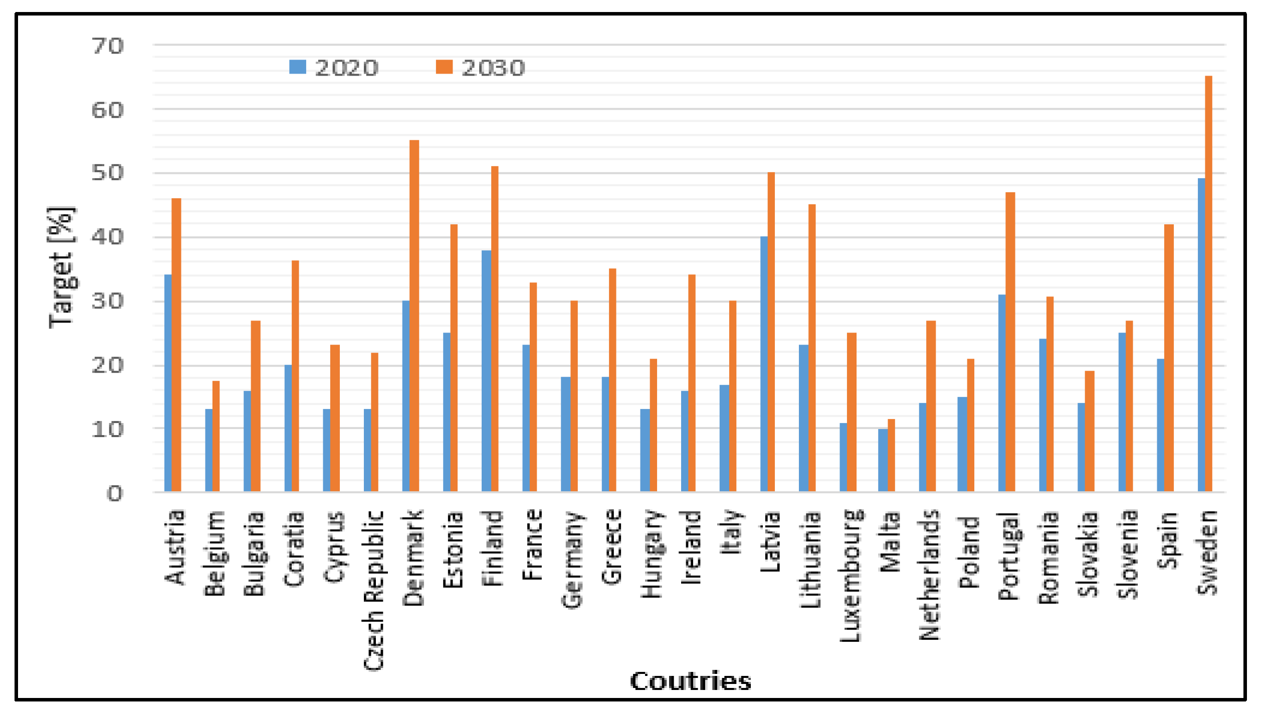
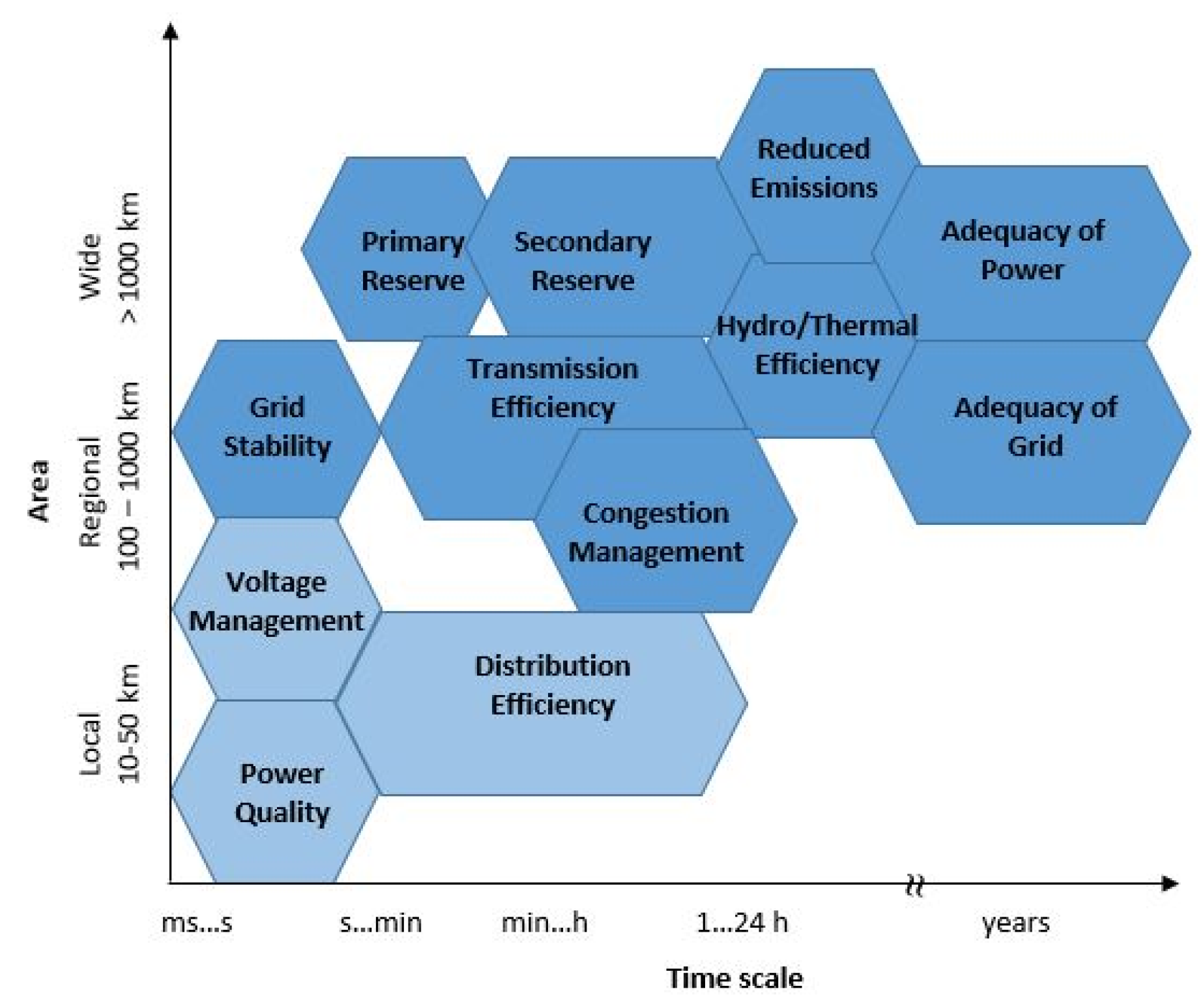
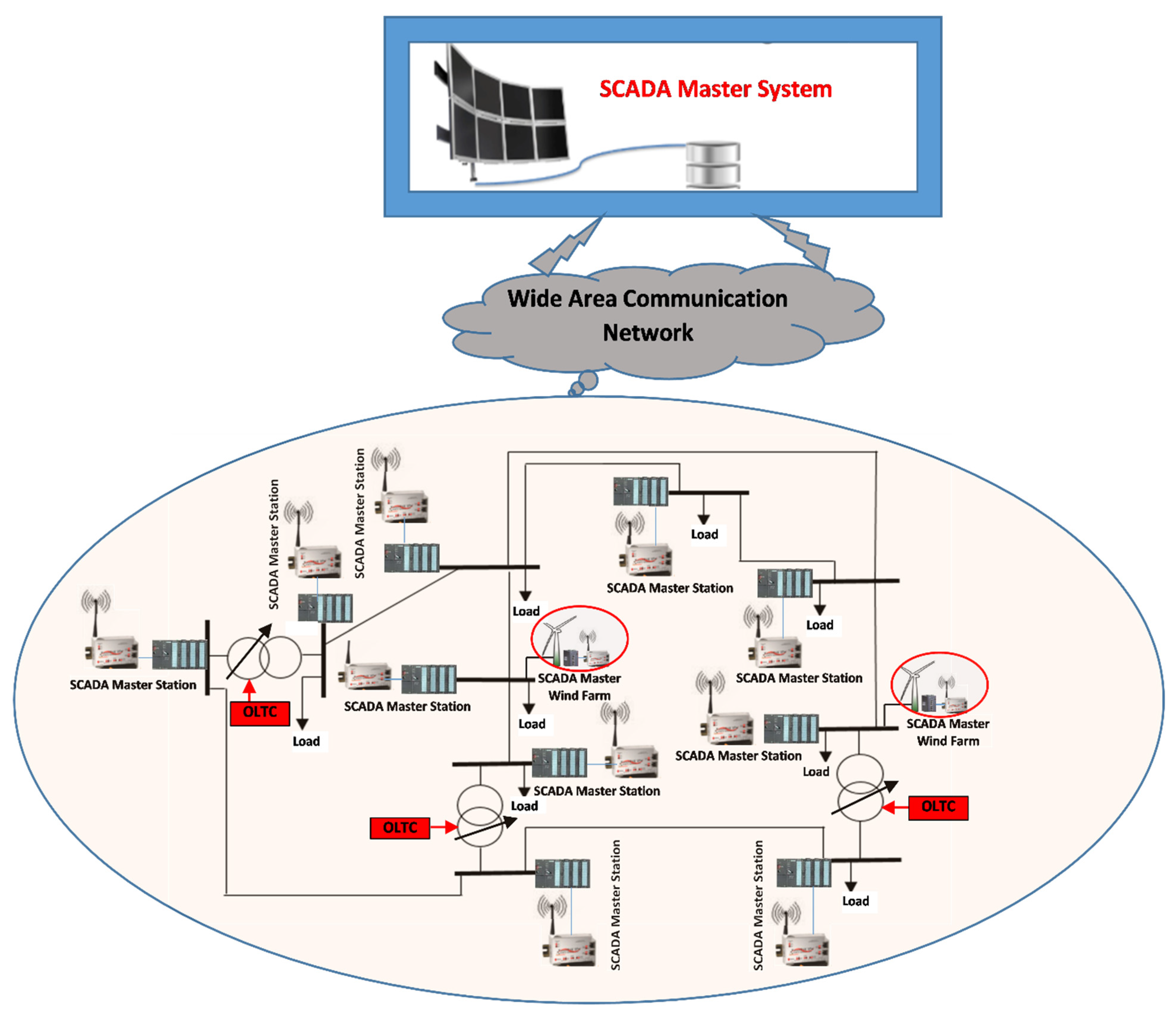
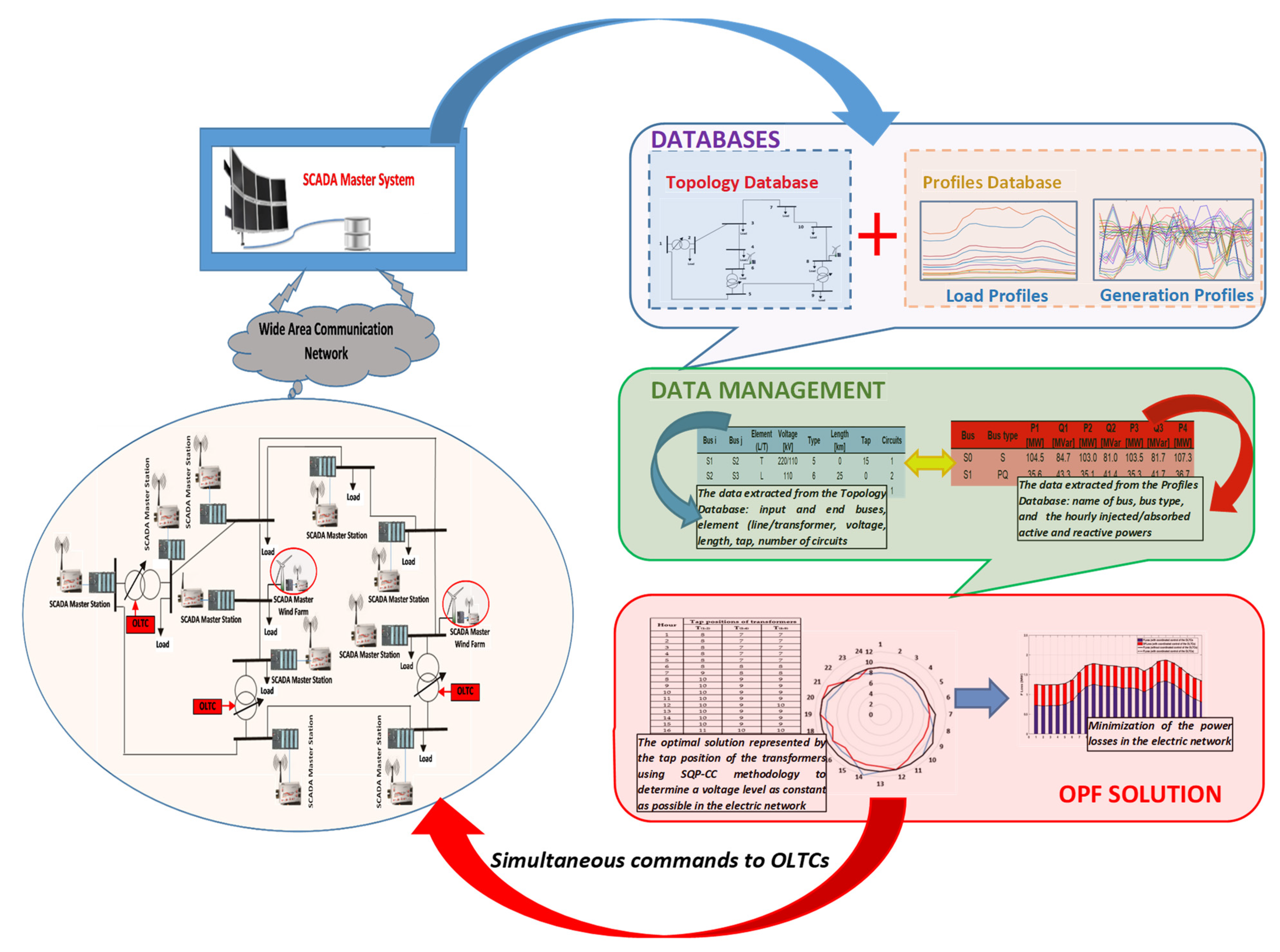
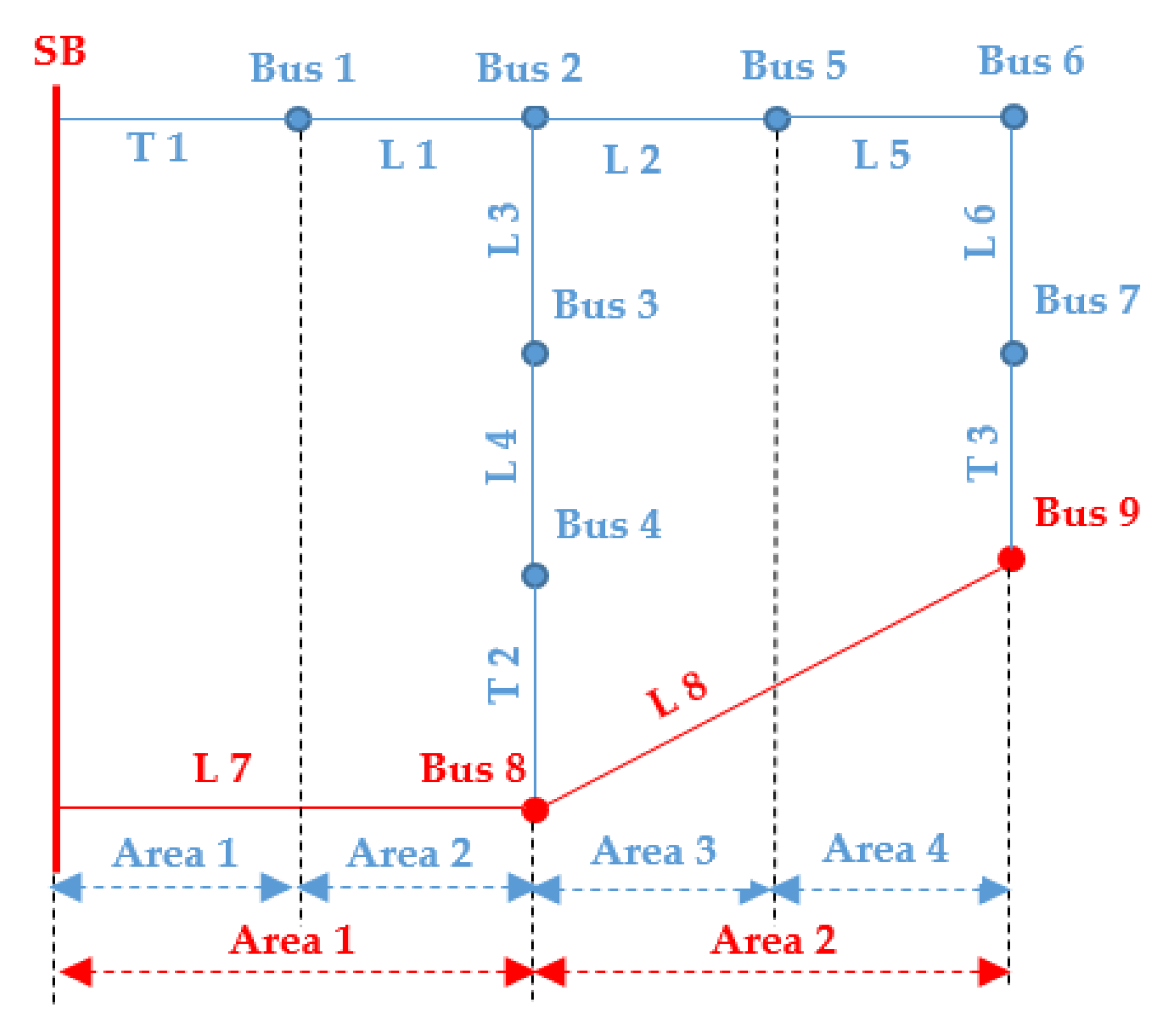


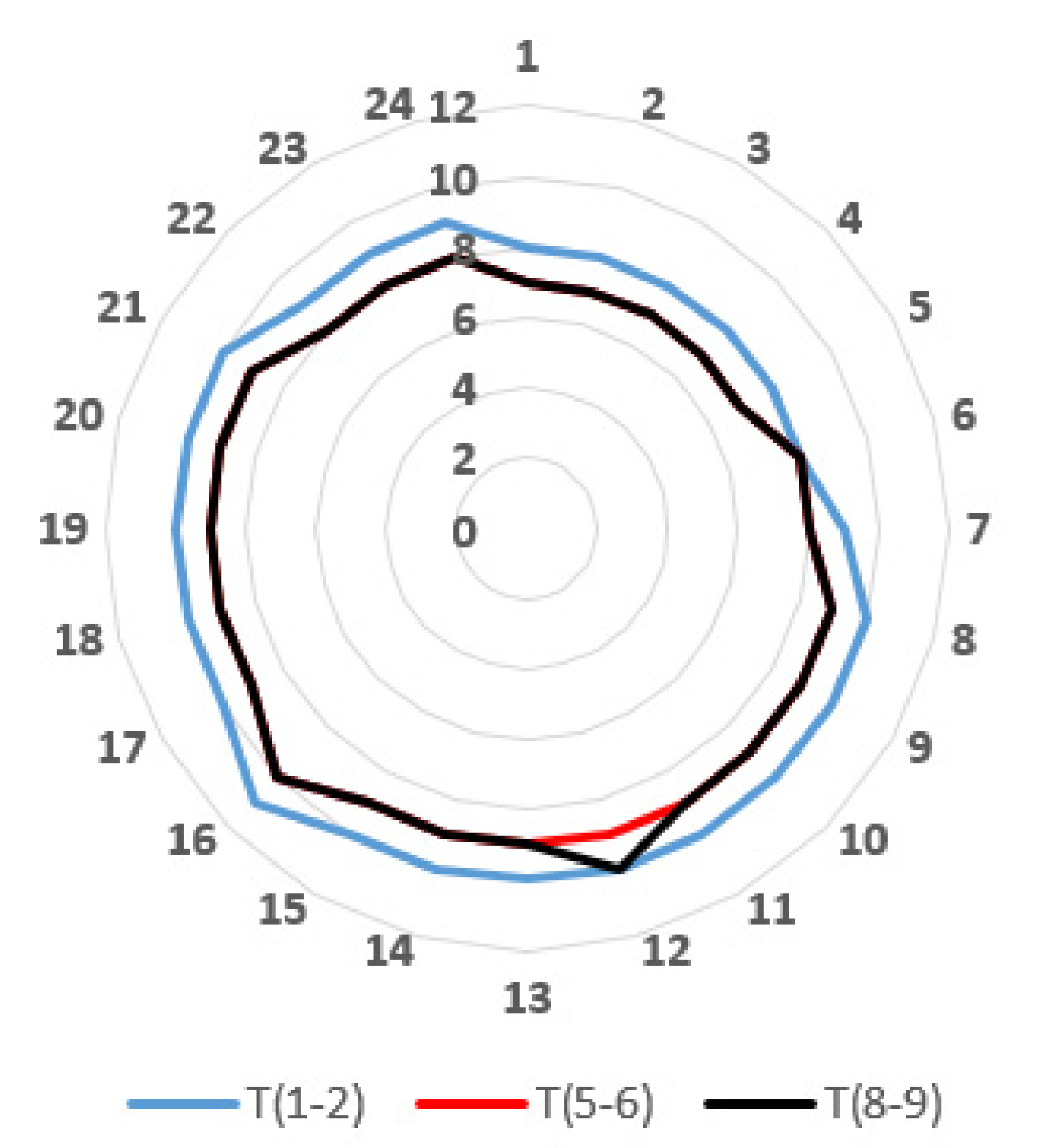
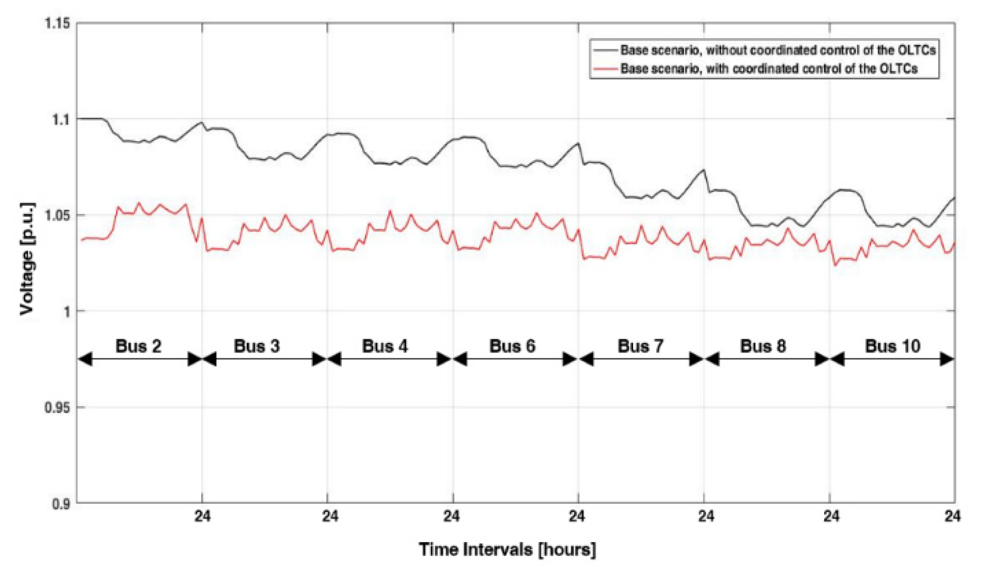
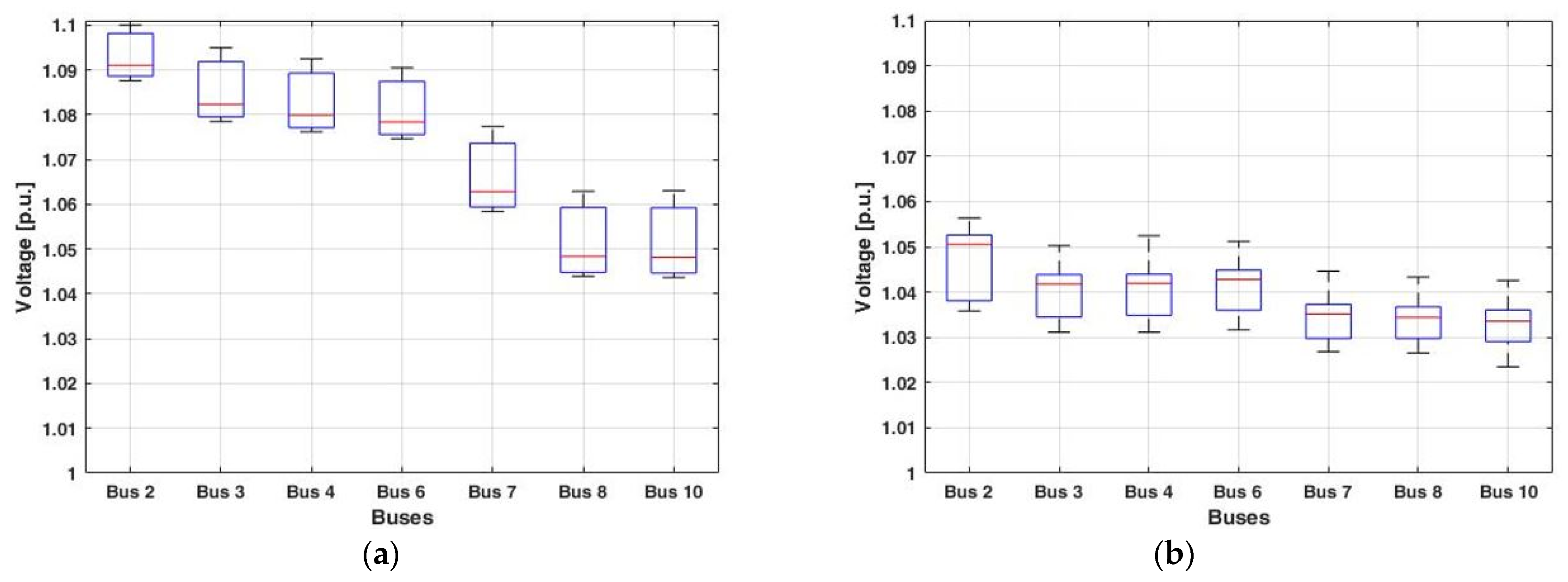
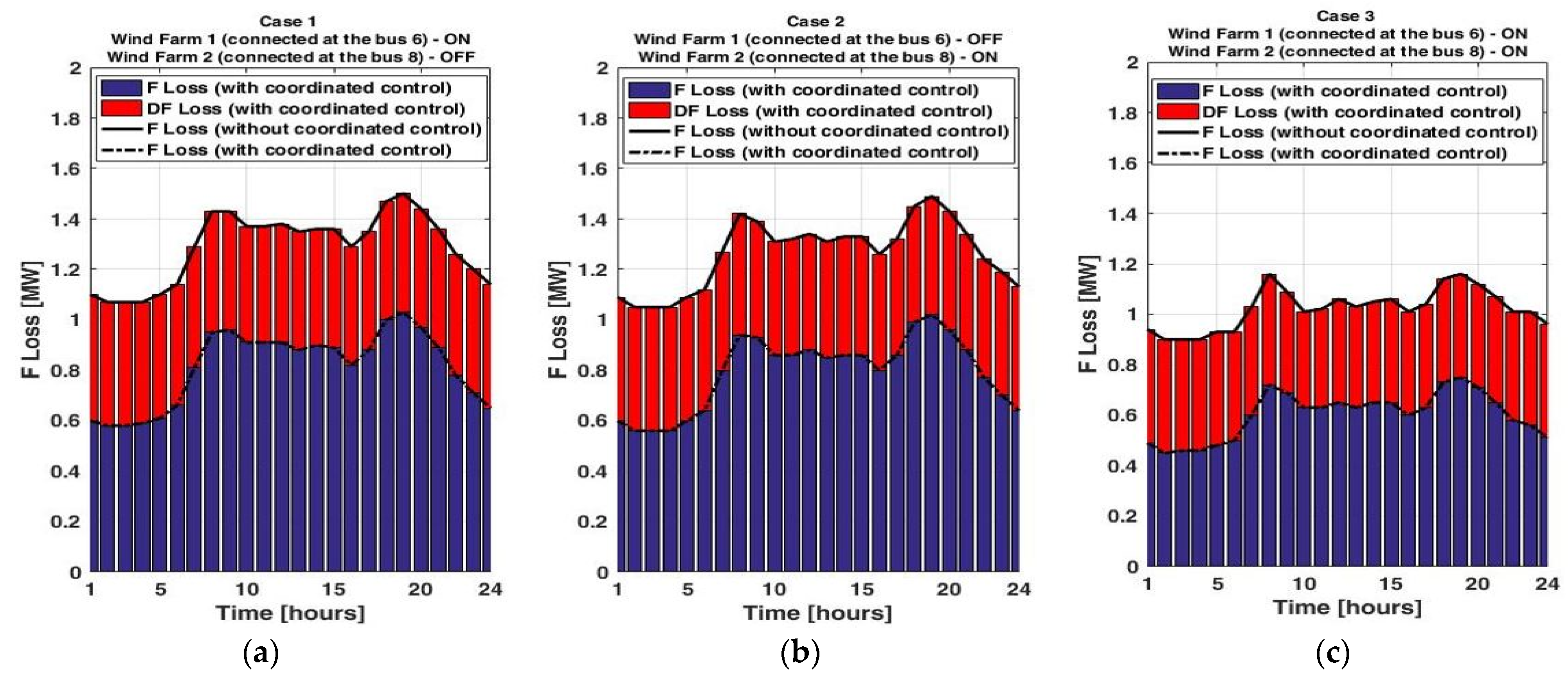

Publisher’s Note: MDPI stays neutral with regard to jurisdictional claims in published maps and institutional affiliations. |
© 2022 by the authors. Licensee MDPI, Basel, Switzerland. This article is an open access article distributed under the terms and conditions of the Creative Commons Attribution (CC BY) license (https://creativecommons.org/licenses/by/4.0/).