Abstract
This study aims to calibrate and validate the EPA Storm Water Management Model from field measurements of rainfall and runoff, in order to simulate the rainfall-runoff process in an urban watershed of Tehran metropolis, Iran. During and after three significant storm events, the flow rates, total suspended solids (TSS), total phosphorus (TP), and total Kjeldahl nitrogen (TKN) concentrations were measured at the outlet of the catchment, and were used in the model calibration and validation process. The performance of the SWMM model was evaluated based on the statistical criteria, as well as graphical techniques. In this study, a local sensitivity analysis was carried out to identify the key model parameters, show that “the percentage of impervious surface in each subwatershed had the most effect on the model output”. Based on the analysis of the results, SWMM model calibration and validation can be judged as satisfactory, and the goodness-of-fit indices for simulating runoff quality and quantity are placed in acceptable ranges. The adjustment obtained for the variations in the measured and simulated flow rates, pollutograph concentrations, total pollutant load, peak concentration, and the event mean concentration (EMC) confirms the considerable predictive capability of the SWMM model when it is well calibrated by using field measurements.
1. Introduction
Urbanization contributes to the development level of a country [1]. Rapid urbanization and the increase in impervious surface areas in urban regions could increase runoff volume by two to six times that of normal runoff [2,3]. Continued urbanization and development also increase the potential for floods, and can cause intensive water quality degradation by increasing associated pollutants, such as suspended solids, fine particles, heavy metals, nutrients, and organic chemicals [4,5,6,7,8], which can all seriously impact public health and threaten environmental quality [9]. Stormwater runoff quantity and quality management for urban regions is a complex task, which has become an increasingly important environmental issue for urban communities [10]. The management of stormwater runoff requires the monitoring and analysis of constituents entering the system, and subsequent implementation of preventive measures [11]. Although effective, extensive monitoring campaigns are not always feasible, due to resource availability and the associated uncertainties. In such a situation, stormwater modelling is a useful tool, which uses limited data resources and can simulate time intervals beyond the monitoring period [12]. Models applicable to managing stormwater quality and quantity appeared in the early 1970s [13,14]. Based on the reviews conducted on the stormwater models by Elliott and Trowsdale [15], and Jayasooriya and Ng [16], the EPA-SWMM model has been effective in stormwater quality and quantity simulation. The SWMM model is a water quality and quantity model widely used in predicting flows and pollutant concentrations, with the capacity for both single-event and continuous simulation [17]. However, the accessibility of suitable data is limited, especially for urban areas, and, as a consequence, parameterization of the model is hindered; therefore, model calibration and validation are in need [18]. Adequate and successful application of a hydrological model can only be reached through efficiently calibrating the model parameters [19]. Normally, model calibration and validation are required prior to regular application of the model to similar site conditions [20].
Application and validation of the SWMM model have been carried out in different parts of urban watersheds around the world [21,22,23,24,25,26,27,28,29,30,31,32,33,34,35,36]. Many studies have shown that the SWMM model has reasonable accuracy when the model outcomes are calibrated and validated [16,17,34,37,38,39,40].
The objectives of this study include conducting a sensitivity analysis on the input parameters of the SWMM model, and calibration and validation of the SWMM model for an urban watershed located in District 22 of Tehran, in order to model the quality and quantity of stormwater runoff. The application of the SWMM model in the study watershed will be helpful in assessing the performance of drainage systems, finding solutions to deal with flood issues, and designing monitoring strategies to manage stormwater in urban watersheds.
The accessibility of the SWMM model input parameters, especially the input parameter values of different pollutant types in different types of land uses for runoff quality modelling, is limited. Due to research gaps, in the present paper, we propose a set of model input parameters that are useful for applying SWMM in similar urban watersheds worldwide.
2. Materials and Methods
2.1. Study Area Description
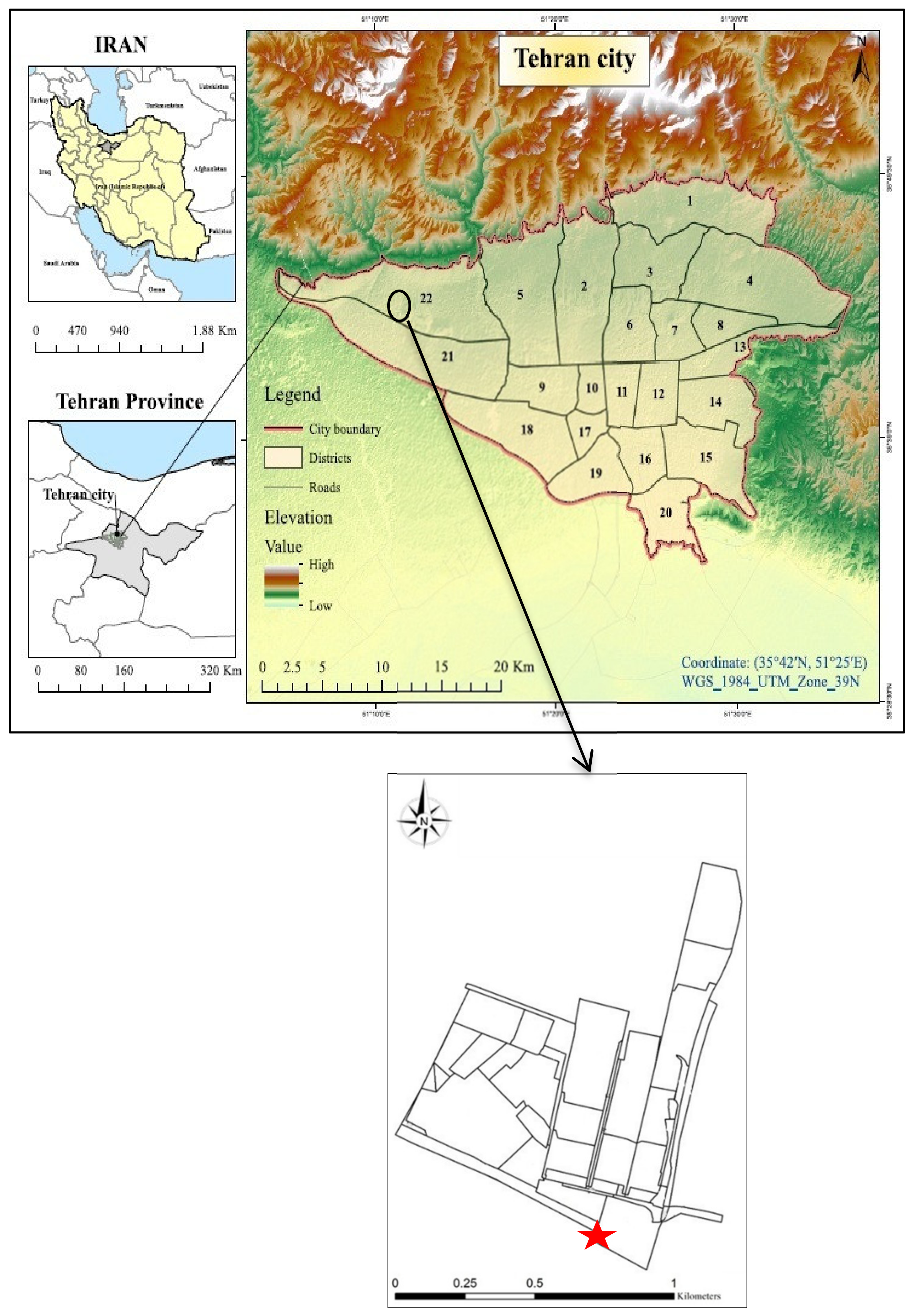
Tehran, as the capital of Iran, is one of the most populous metropolises in the world. District 22 of Tehran municipality is one of 22 urban districts of Tehran with geographical coordinates of 35°32′16″–35°57′19″ north latitude and 51°5′10″–51°20′40″ east longitude, and with an area of 24,000 ha. The study watershed is located in the southern part of District 22 of Tehran (Figure 1). The total watershed area is about 95 ha, mainly comprising residential, commercial and undeveloped areas. The mean annual precipitation in the study area is 238.9 mm, and the main part of rainfall occurs during fall and spring seasons. The elevation change throughout the landscape is gentle, ranging from 1284 m in the north to 1226 m in the south, which gives a mean slope of approximately 8%. All of the subwatersheds had separate sewage drainage systems, and the stormwater runoff flowed past conduits to the final outfall.

Figure 1.
Location of District 22 of Tehran, the study watershed and its sub-watersheds (star marks the outlet location of the study watershed).
2.2. Description of Storm Events and the Corresponding Runoff Monitoring
The aim of this study was to calibrate and validate the SWMM model by using measurements of runoff and pollutant concentration. The runoff discharge and quality were monitored for the three recorded storm events at the end of the drainage network of the study watershed (on 22 May 2018, 1 June 2018, and 14 November 2018). Flow rates were measured by the cross-section method and water samples were collected at 10 min time intervals at the watershed outlet cross-section for analyzing water quality. In this analysis, three pollutants of total suspended solids (TSS), total phosphorus (TP), and total Kjeldahl nitrogen (TKN) were employed for calibration and validation of the SWMM model. A total of 59 samples were taken during and after three storm events occurred during the study period. The samples were stored in 1 L bottles at the site and transported to the laboratory at Tehran University. Chemical analyses were performed by standard methods (TSS, TP and TKN concentrations were measured using gravimetric method, yellow colorimetric method, and Kjeldahl method, respectively). In addition, 10 min storm data collected from Mehrabad synoptic weather station, which is located near the study area, were used in this study. The main characteristics of the storm events are summarized in Table 1.

Table 1.
Main characteristics of the studied storm events.
2.3. SWMM Model Description
The SWMM model is a dynamic event-based rainfall-runoff model for long-term simulation of runoff quantity and quality, particularly in urban watersheds, and the first version of the model was introduced by the U.S. EPA in 1971 [41] and has been very popular in urban water resource management since then. A broad range of studies have been undertaken on SWMM-based simulation of runoff quantity and quality dynamics, including hydrologic assessment for pre- and post-development conditions [27], pollutant wash-off water quality analyses [28,34,35], combined sewer overflow modelling and assessment [42], flood forecasting [43], and modelling and assessment of stormwater treatment facilities [44,45]. The model has computational blocks to perform rainfall-runoff modelling. Runoff block generates runoff from rainfall using the non-linear reservoir method, which assumes subcatchment as a non-linear reservoir. Overland flow from each subcatchment is computed by applying the law of conservation of mass [46]. Transport and EXTRAN blocks route the runoff flows through storm water drains using kinematic and dynamic wave routing, respectively. Infiltration can be estimated using the Soil Conservation Service curve number (SCS-CN), Horton, modified Horton, and Green and Ampt methods. For each model run, all computational blocks can work simultaneously or individually [39]. In the present study, the kinematic wave routing method with 1 s time steps and the SCS-CN method were used for flow routing and infiltration, respectively. SWMM is enabled to simulate pollutant delivery by using buildup and wash-off equations. Perfectly parameterizing the equations for different land uses is of importance for utilizing the full potential of SWMM. Three buildup equations (power, exponential, and saturation) and three wash-off equations (exponential, rating curve, and event mean concentration) are provided in SWMM [41]. In this study, power and exponential equations were used to simulate buildup and wash-off of the pollutants, respectively. The equations are as follows [47]:
where Buildup is pollutant build-up (mass per unit of curb length), and and are maximum possible build-up (mass per unit of curb length) and build-up rate constant, respectively. t denotes time and represents time exponent.
where the wash-off term is the wash-off load (mass per hour), the runoff term is runoff rate per unit area (inches/hour or mm/hour), and Buildup is the pollutant buildup in units of total mass. is the wash-off coefficient, and is the wash-off exponent.
2.4. Model Parameterization
EPA SWMM model was set up based on the topographical and drainage network data and parameters derived based on the properties of the subcatchments [48]. In this study, the initial input parameter values were estimated through a combination of field data, existing datasets, literature review, and model default values. The spatial degree of segmentation of a subcatchment, which represents the surface hydrologic characteristics, is very important in SWMM-based modelling of urban runoff [49]. The catchment was segregated based on the hydrologic conditions as a hydrologic similar unit (HSU) or subcatchment, via land use and surface slope condition, considering drainage network. Catchment delineation and subdivision was successfully performed and 42 subcatchments were extracted, which indicates a fairly detailed discretization. A field survey was also carried out to confirm the surface and subsurface drainage patterns to accurately describe the subcatchment physical characteristics. The physical characteristics of the subcatchments, including areas, average surface gradients, overland flow path widths, and grade of impermeability, were calculated accordingly, based on digital elevation model (DEM) data with a resolution of 3 m × 3 m, using ArcMap, field measurements, and available equations, in addition to the existing data, such as land use and soil data, while typical values from the literature review were taken for the Manning’s roughness coefficients of pervious and impervious areas, for depression storage depths of pervious and impervious areas, and for % impervious areas with zero depression storage. Curve number (CN) values were assigned for each drainage area within the catchment. The main significant variables for defining a curve number are the soil hydrologic group and cover type. In order to determine CN values for the impervious areas and the pervious soil, the soil hydrologic groups and cover types for each drainage area were determined from the existing land use and soil maps obtained from municipal offices. The spatial distribution of 188 conduits, and then their geometries and properties (conduits lengths, conduits depths, conduits widths, down and up stream invert levels and invert slopes), were determined based on the drainage network map collected from the municipal offices in digital format and via field measurements, while typical values for the Manning’s roughness coefficient for the conduits were extracted from the literature review. The spatial distribution of 244 junctions and their physical parameters, including junctions’ invert elevations and junctions’ maximum water depths, were prepared based on the 1:2000 CAD format topographic map collected from Iran National Cartographic Center, the existing datasets of drainage network, and field measurements. Subsequently, the parameters of each subcatchment, each channel and each junction were imported into the simulation tool of SWMM, and the connections among subcatchments, junctions, conduits, and outlets were configured according to their spatial positions.
The major limitation of catchment water quality modeling is the proper identification of the land use for each catchment, which controls the transport of pollutants with stormwater runoff [50]. The land use information was extracted from the land use thematic map (2016) collected from the municipal offices and according to field observations applied to SWMM. In SWMM, for each type of pollutant, each land use has a unique set of pollutant parameters, i.e., four parameters for each land use. Initial values for these parameters were employed, according to the literature review. Initial values of model input parameters for runoff quality modelling in 5 different types of land uses related to the study region (including low-density residential, high-density residential, commercial, undeveloped, and roads) were extracted from the literature review, as given in Table 2. In addition, the previous conditions of the catchment area, such as the number of previous dry weather days and street sweeping data, were imported into the model to simulate pollutographs.
Table 2.
Initial values of the quality parameters of TSS, TKN and TP used for runoff quality calibration of the SWMM model.
2.5. SWMM Model Sensitivity Analysis
The assessment of model output through changes in parameter values is performed with a parameter sensitivity analysis. Sensitivity analysis is conducted for a variety of reasons, such as identification of parameters that require additional investigation for fortifying the knowledge base, thereby decreasing output uncertainty; determination of insignificant parameters to be removed from the final model; identification of inputs that contribute most to output variability; determination of parameters that are most highly correlated with the model output [59]. In modelling, the parameter sensitivity analysis indicates the parameter robustness [48]. In this study, the sensitivity of the model inputs or parameters to the SWMM model output was examined to identify key parameters. Sensitivity analyses can be broadly grouped into local and global approaches [60]. In this article, local sensitivity analysis was carried out. Following techniques employed by Jewell et al. [61,62,63,64,65,66,67], input parameters of SWMM model (as listed in Table 3) were justified over a range of ±50% of their original values, while keeping all other parameters constant, and the corresponding difference in runoff peak flows was calculated.
Table 3.
The final values of the main calibrated parameters of the SWMM simulation model.
As a result, the parameters for which small variations in their values lead to significant changes in the model output were selected and ranked by efficiency for further analysis. In other words, the highest sensitive parameters were employed while conducting the SWMM model calibration.
2.6. SWMM Model Calibration and Validation
In order to simulate accurate scenarios of runoff generation and pollutant loading with urban storm water by using the calibrated and validated SWMM model, in this study, two storm events (22 May 2018 and 14 November 2018) were used for the model calibration, and one storm event (1 June 2018) was used for the model validation. According to the measurement data, the optimal values of the sensitive parameters were determined by carefully adjusting the most sensitive parameters of the model in well-defined ranges for ensuring the simulation validity. The parameters of the SWMM model considered for calibrating the runoff quantity, and their variation ranges, and the values chosen for these parameters in this study, are given in Table 3. The model calibration was performed through a trial-and-error iterative process, by adjusting the parameters within the established ranges, as represented in Table 3. The parameters were systematically adjusted one at a time until differences between the modelled and measured values were minimized. In other words, the calibration process for a parameter was completed when the modelled results closely matched the measured values. Calibration of the SWMM model for runoff quality was conducted in terms of four parameters for each type of pollutant in each landuse (Blim, Bexp, WC and Wexp). During the calibration process of SWMM, each parameter was adjusted within a certain range until good agreements were gained between the measured and simulated pollutographs, with respect to total pollutant load, peak concentration, and the event mean concentration (EMC) values.
The main objective of model validation is to confirm whether the set of calibrated parameters enable other storm events to be simulated in the future [48]. The mean values for calibrated parameters (two storm events on 22 May 2018 and 14 November 2018), in order to simulate the runoff quantity and quality, were then used to validate the model, and the hydrograph and pollutographs of the storm event on 1 June 2018, gained from each simulation, were compared with the measured hydrograph and pollutographs (numerically and graphically).
2.7. Goodness-of-Fit Test
The model performance during the calibration and validation stages was evaluated graphically and also statistically using goodness-of-fit indices as suggested in the literatures [24,62,63,64,65]. Five statistical criteria considered for evaluating the model performance include the Nash–Sutcliffe efficiency coefficient (NSC), coefficient of determination (R2), RMSE-observations standard deviation ratio (RSR), percent bias (PBIAS), and relative error (RE). Details of these criteria are as follows:
Interpretation of the goodness-of-fit parameters for the model calibration and validation stages was conducted according to Moriasi et al. [65]. Table 4 gives the qualitative performance rating system employed to evaluate the performance of the SWMM model.
Table 4.
Model performance rating system [65].
3. Results and Discussion
3.1. Sensitivity Analysis Results
In order to identify the sensitive parameters affecting the model output (runoff peak flow), a sensitivity analysis of the nine various parameters (as given in Table 3) was performed in this study. For this purpose, the initial values of the input parameters were varied within ±50% ranges and the percentage rate of changes in the model output were considered. In total, the SWMM model was run 90 times. As illustrated in the modelling results, the percent of impervious area (%Imp.) and the average surface slope of the subcatchment were the highest and the lowest sensitive parameters in the determination of the peak flow rate, respectively, which indicates that the percentage of imperviousness regulates the peak flow rate in the hydrograph and the average surface slope of the subcatchment has weak connections to the model predictions. As the percent of impervious area and the average surface slope were varied within −50% to +50% ranges, the percentage rate of changes in peak flow were from −22.43% to 21.50% and −0.084% to 0.017%, respectively. Temprano et al. [34], Tan et al. [33], Chow et al. [24], and Maharjan et al. [17] found a similar influence for %Imp. The ranking of the parameters’ influence on the mentioned output was the percent of impervious area (%Imp.), SCS runoff curve number, depth of depression storage on the impervious area (Dstore-Imperv.), width of the overland flow path, Manning’s coefficient for overland flow over the impervious portion of the subcatchment (N-Imperv.), percent of impervious area with no depression storage (%Zero-Imperv.), and the average surface slope, respectively. As we changed these subcatchment parameters (%Imp., CN, Dstore-Imperv., width, N-Imperv., %Zero-Imperv. and %slope) within −50% to +50% ranges, the percentage rate of changes in peak flow were from −22.43% to 21.50%, 0% to 7.85%, 0.17% to −0.78%, −0.31% to 0.023%, 0.023% to −0.11%, −0.06% to 0.04%, and −0.084% to 0.017%, respectively. According to the results, as the depth of depression storage on the impervious area (Dstore-Imperv.) and Manning’s coefficient for overland flow over the impervious portion of the subcatchment (N-Imperv.) increased, the peak flow decreased, which is similar to the findings by Chow et al. [24]. In addition, as the average slope, flow width, percentage of impervious area, and percent of impervious area with no depression storage of the subcatchment and SCS curve number increased, the peak runoff also increased. The results of the sensitivity analysis in this research confirm that in the area, the runoff peak value simulated by SWMM was the most sensitive to change in the properties related to the imperviousness, in particular, the percent of impervious area, depth of depression storage on the impervious area, Manning’s roughness coefficient over the impervious portion, and percent of impervious area with no depression storage, respectively. According to the results, the Manning’s roughness coefficient for overland flow over the pervious portion of the subcatchment (N-Perv.) and the depth of depression storage for the pervious area (Dstore-Perv.) have no effect on the peak runoff estimation modelled by SWMM; Moafi Rabori et al. [66] found similar results.
3.2. Model Calibration Results
3.2.1. Runoff Quantity
For the purpose of catchment modelling system calibration, the relevant SWMM model parameters were adjusted (according to their sensivity degree, systematically), and the model was evaluated for the modelling capabilities through four indicators using Equations (3)−(6). In Table 4, the average values (between the following two calibration rainfall events: 22 May 2018 and 14 November 2018) of the main calibrated parameters for runoff quantity are reported.
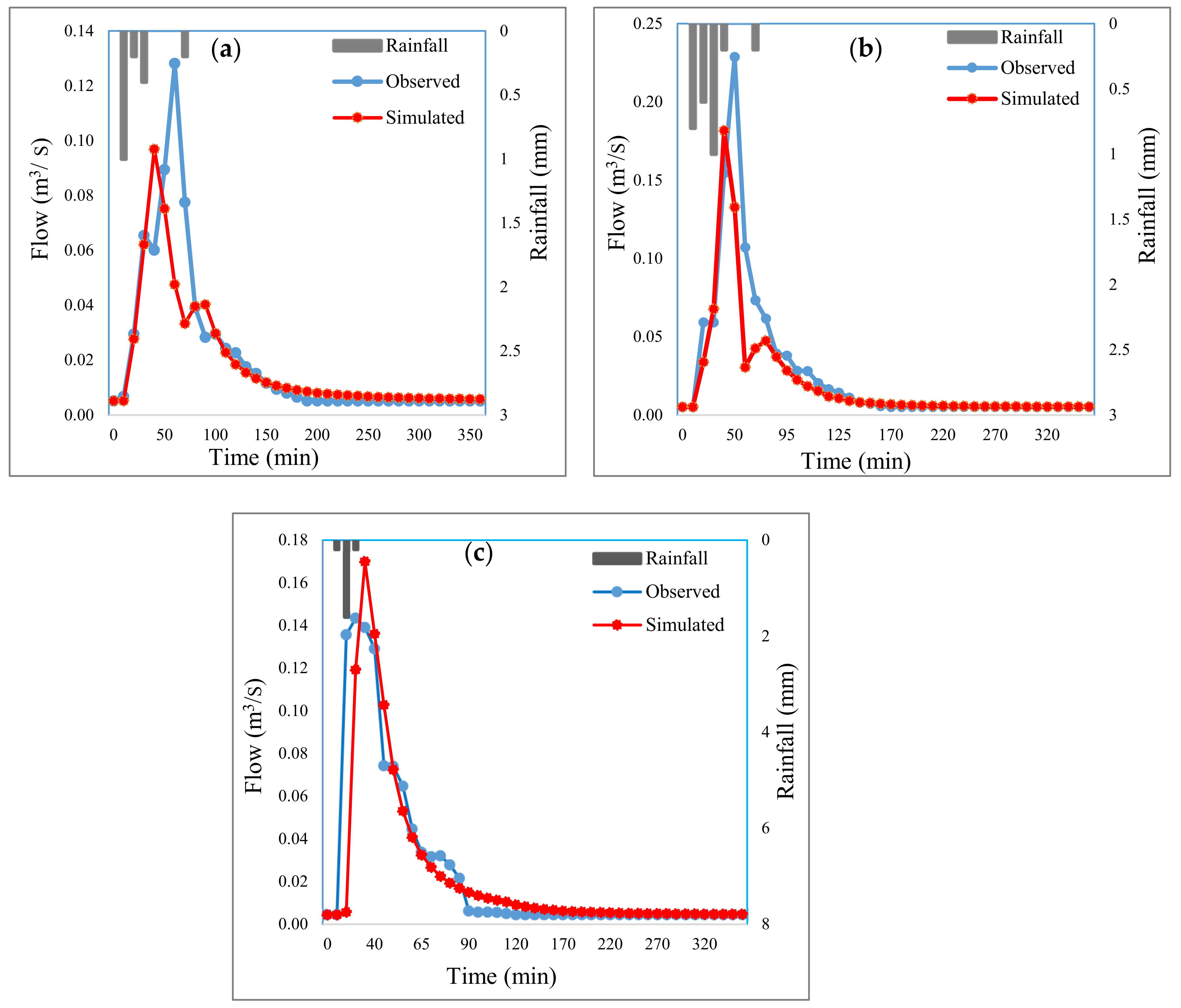
During calibration, the simulated runoff rates showed an overall good relationship with the measured values for two events (22 May 2018 and 14 November 2018 rainfall events) at the outlet in the catchment. Figure 2a,b show a comparison of the modelled and monitored discharge values for the two rainfall events investigated. Generally, as we can observe in Figure 2a,b, a visual comparison between the calibration hydrographs demonstrated acceptable fit between the observed and simulated data, although some differences in timing and/or magnitude were observed.

Figure 2.
Comparison between observed flow hydrograph (blue line) and simulated flow hydrograph (red line) for the first two events employed for model calibration, (a) 22 May 2018 and (b) 14 November 2018, and the third event employed for model validation, (c) 1 June 2018.
The total simulation accuracies of all the tested events were also assessed by statistical parameters. The goodness-of-fit test results for the calibration step are summarized in Table 5. For the event on 22 May 2018, the value of NSC was 0.65, i.e., greater than 0.50, R2 was 0.65, i.e., greater than 0.6, RSR was 0.59, i.e., less than 0.70, and PBIAS (%) was 9.61%, i.e., less than +15%; for the event on 14 November 2018, the value of NSC was 0.78, i.e., greater than 0.65, R2 was 0.81, i.e., greater than 0.8, RSR was 0.47, i.e., less than 0.55, and PBIAS (%) was 22.05%, i.e., less than +25%; according to Moriasi et al. [65], indicating the model performance was deemed acceptable for flow discharge simulation of the two calibrated events at four important indicators, and the model is considered well calibrated for estimating the runoff quantity at the catchment scale. Baek et al. [67] and Niyonkuru et al. [48] found similar results, and in their works, the values of the testing parameters from the quantity calibration were reasonable and in acceptable ranges.
Table 5.
Summary results of goodness-of-fit test for assessing the reliability of SWMM model calibration and validation phases for runoff quantity simulation.
3.2.2. Runoff Quality
After testing the goodness of fit in the quality calibration step, with the rainfall events on 22 May 2018 and 14 November 2018, for the TSS, TP and TKN pollutants, the best-fit values for the input build-up and wash-off parameters were obtained. Table 6 presents the average resulting calibrated values for the input parameters of quality modelling in each land use and for all the pollutants monitored.
Table 6.
Optimal build-up and wash-off input parameters of the water quality module in the SWMM model.
Based on this calibration process, according to the values of the NSC, R2, RSR and PBIAS (%) indicators obtained using Equations (3)−(6) for the calibrated events on 22 May 2018 and 14 November 2018, the accuracy of the adjustment of the TSS, TP and TKN measured and simulated pollutographs, at the exit of the catchment area during the two rainfalls analysed, was considered acceptable [65], as Table 7 points out.
Table 7.
Summary results of goodness-of-fit test for assessing the reliability of SWMM model calibration and validation phases for runoff quality simulation.
For the quality calibration, the NSC, R2, RSR and PBIAS (%) values ranged from 0.60 to 0.72, 0.68 to 0.82, 0.53 to 0.63, and −6.99 to 16.71, respectively.
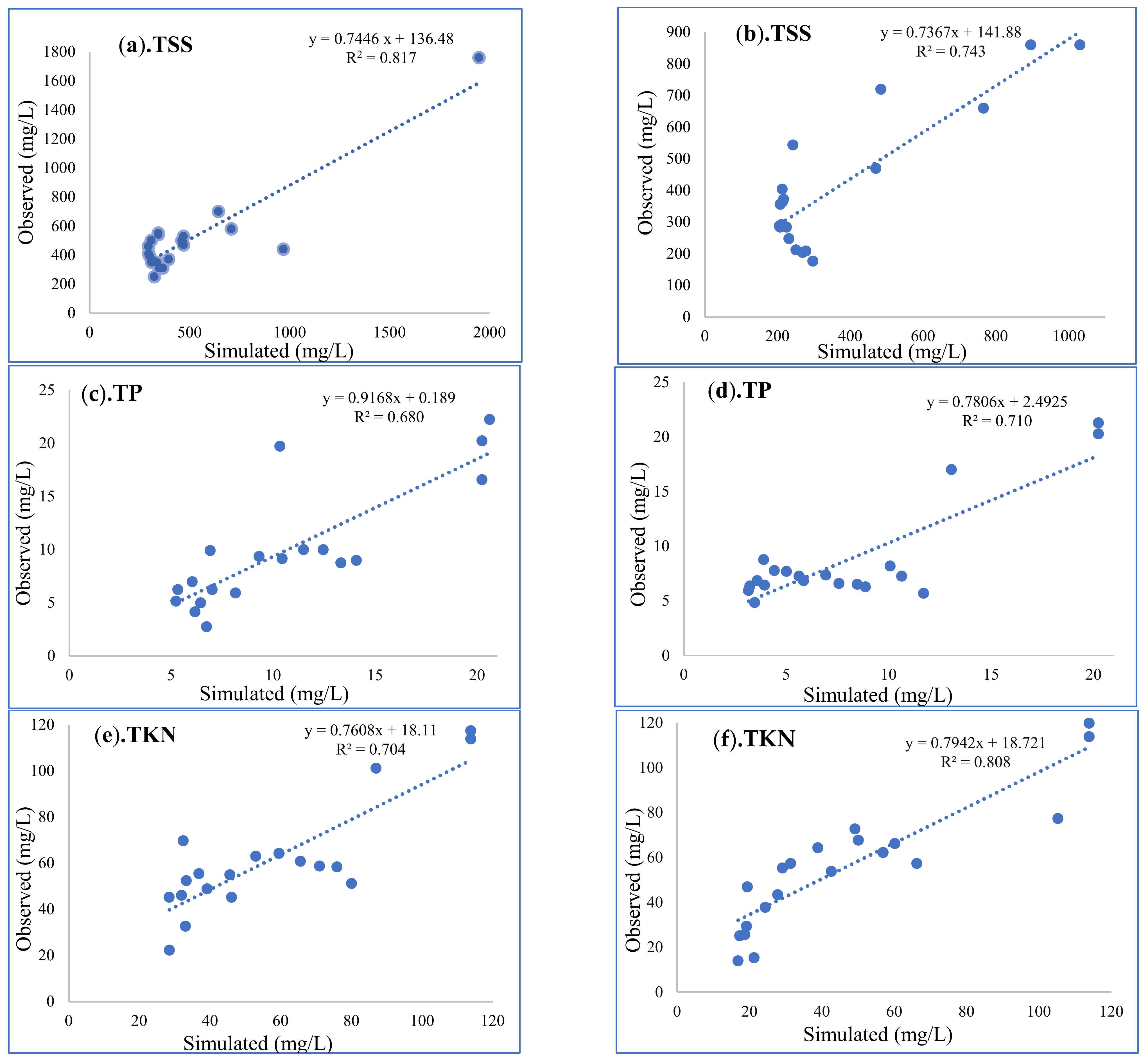
The goodness of fit was also assessed by plotting the simulated versus observed values of pollutant concentrations, as shown in Figure 3a–f. In this figure, a linear regression line of the form yp =·yo (where yp implies a predicted value and yo implies an observed value) was fitted through the data, and its slope was compared with the 1:1 slope (perfect match). The value of the slope is a measure of the over- (slope greater than 1.0) or under-prediction (slope less than 1.0) of the model compared with the observed data. In addition, the square of the correlation coeffcient (R2) of the regression line is presented in the figure. The lower the value of R2 (below 1), the worse the data correlates with the regression equation. Therefore, the best verification requires that the values of both and R2 be as close to 1.0 as possible [35]. All the slopes () of the calibrated events in the TSS, TP and TKN simulations were close to 1.0 (less than 1.0) and ranged from 0.74 to 0.92; this means that the modelled pollutant concentrations corresponded well with the measured pollutant concentrations, and were generally slightly under-predicted. These deviations can be attributed to the errors in the measured values. The R2 values obtained in the correlations for the event on 22 May 2018 were 0.82, 0.68 and 0.70 for the TSS, TP and TKN modelling, respectively (all greater than 0.6); the R2 values for the event on 14 November 2018 were 0.74, 0.71 and 0.81 for the TSS, TP and TKN simulations, respectively (all greater than 0.7), which can be regarded as acceptable performance.

Figure 3.
Correlation between measured and simulated concentrations of the pollutants for the following calibration rainfall events: (a,c,e) 22 May 2018; (b,d,f) 14 November 2018.
As Table 8 presents, the application results were compared and analyzed in terms of the loadings of TSS, TP and TKN, the peak concentrations of TSS, TP and TKN, and the event mean concentrations (EMCs) of TSS, TP and TKN. Except for the loadings of TKN in both the calibrated events, the loadings of TP, and the EMC of TKN in the event on 14 November 2018, the other results showed that the RE% values of the simulated pollutographs were nearly in the range of ±30% of the observed pollutographs, in a range from −19.86% to 27.17%, indicating that the measures of the simulated curves were an acceptable fit for the observed curves. However, the negative RE% values given in Table 8 show that the SWMM model underestimated the parameters. The stormwater model capability in the calibration phase, for application of the model in the quality simulation of urban areas, has also been investigated by Rezaei et al. [70], who reported that the calibration result was quite satisfactory.
Table 8.
Summary results for assessing the accuracy of the water quality module for simulating EMC, load and peak concentrations of the pollutants for each rainfall event.
3.3. Model Validation Results
The values of the optimized parameters obtained from the calibration of the SWMM model to the two rainfall events were used to simulate the quantity and quality of runoff for the third independent rainfall event, without further adjustment. Based on both graphical and statistical measures, the SWMM model performance was evaluated, indicating a good agreement between the simulated and measured runoff.
The comparison of the simulated and observed runoff hydrographs for the SWMM model validation on 1 June 2018 demonstrated good fitness between the observed and simulated runoff discharge time series, as shown in Figure 2c.
Table 5 represents the efficiency indices employed to assess the validation results of the SWMM model. The results showed that for the hydraulic validation, the values of NSC, R2, RSR and PBIAS (%) were 0.72, 0.73, 0.53 and 6.21, respectively, which were within the acceptable ranges [65], indicating a good relationship between the simulated and observed runoff discharge time series.
As demonstrated in Table 7, for the runoff quality validation, among the concentrations of TSS, TP and TKN measured at the outlet of the study urban catchment, with respect to the model estimates, good fitness was obtained between the simulated and measured values. The SWMM model for runoff quality simulation was acceptable, based on four performance indicators, NSC, R2, RSR and PBIAS (%) [65]. During the runoff quality validation, the NSC values were greater than 0.50, the R2 values were greater than 0.6, the RSR values were less than 0.7, and the PBIAS (%) values were less than +25%. It can be concluded that satisfying results were achieved for runoff quality simulation.
For the SWMM model validation phase, evaluation was also performed by comparing the observed and simulated values of the event-based pollutant loads, peak concentrations, and EMCs for the TSS, TP and TKN pollutants, using their relative error (RE), as given in Table 8. The simulated total loads, peak concentrations, and EMCs only indicated a difference of ±30% of the measured values, ranging from −16.76% to 28.15%, with the exception of the load and EMC of TKN. Thus, the SWMM model enables the processes describing water quality to be mimicked satisfactorily. The main reason for having RE% values beyond the ±30% range, given in Table 8, could be the methods used for the loads and EMCs calculation, and another reason could be the errors in the measured values, which could make a difference between the simulated and observed values.
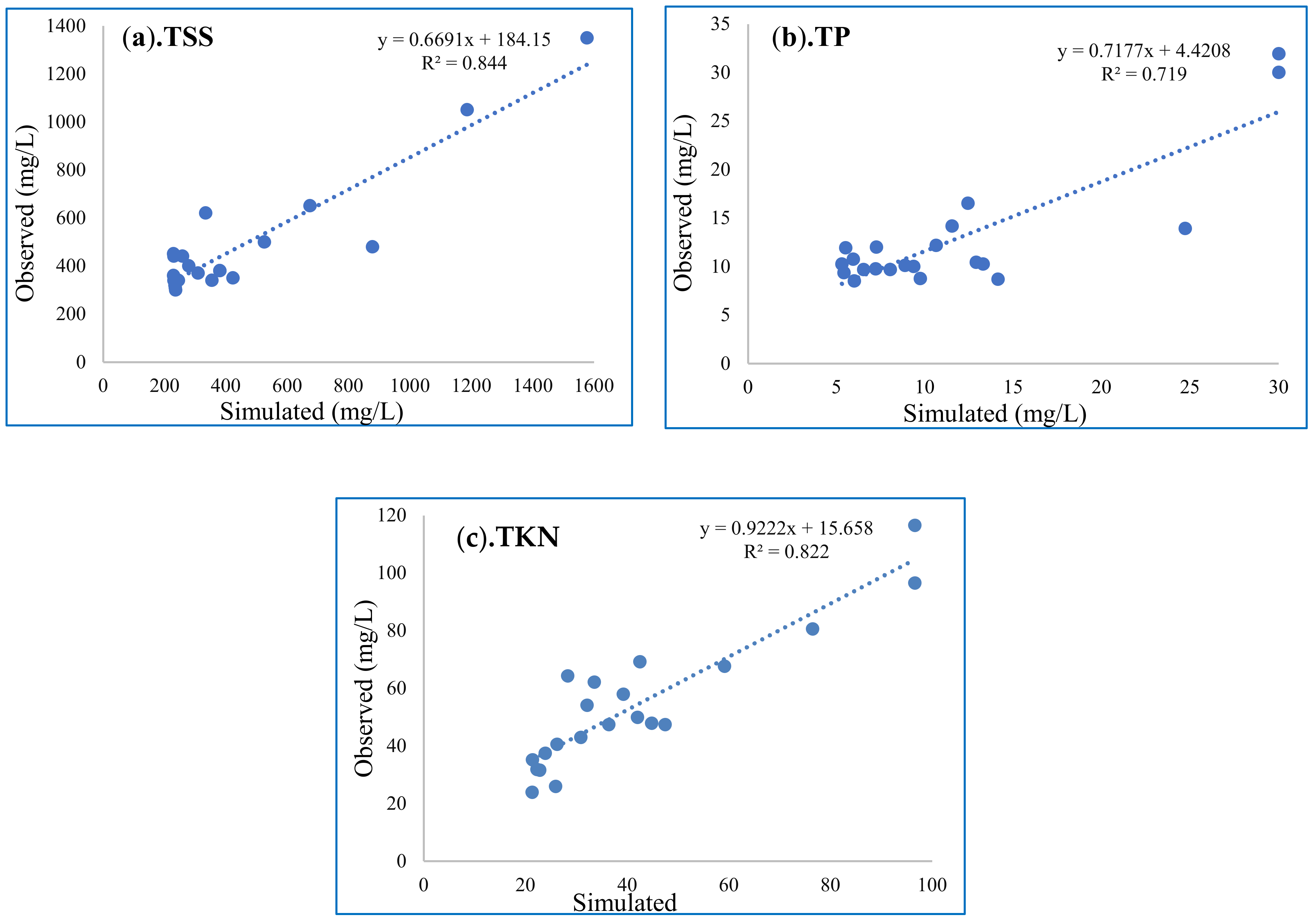
As shown in Figure 4a–c, a regression analysis between the simulated and observed values was used again to assess the SWMM model performance for the validation phase. The correlations between the measured and simulated values of TSS, TP and TKN were determined by the statistical measure of R2, and also the slopes of the best-fit lines on plots of the measured and simulated values. For the event on 1 June 2018, in particular, the R2 values were equal to 0.84, 0.72 and 0.82 for TSS, TP and TKN, respectively. These values are all greater than 0.7; therefore, they have been suggested as acceptable for the model results. The slope values of the regression equations extracted for the validation rainfall event for the TSS, TP and TKN pollutants were 0.67, 0.72 and 0.92, respectively. Despite the slope values being less than one during the validation rainfall event on 1 June 2018, the runoff quality from the study urban catchment was under-predicted. Even though this was the case, the simulated values were well interpolated from the measured values of concentrations of the pollutants (as the slopes coefficients are all close to 1.0).
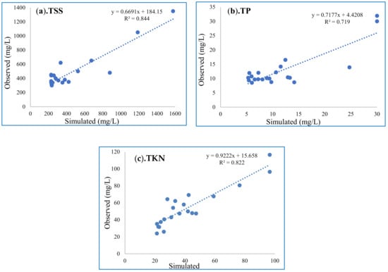
Figure 4.
Correlation between measured and simulated concentrations of the pollutants for the following validation rainfall event: (a–c) 1 June 2018.
Overall, the calibration and verification results indicated that the model structure and parameters matched the runoff-producing pattern, and that the calibrated model was suitable for simulating the rainfall-runoff process in the study urban catchment. In addition, it has been verified that it is likely to obtain a good adjustment, in terms of the variations in flow rates and the pollutants by adequate modification of the parameters that the program gives. The literatures by Ketabchy [71], Alamdari [22] and Hai [25] also showed that the calibrated SWMM model structure and input parameters fitted the observed runoff-producing pattern, and indicated that the SWMM model could sufficiently predict stormwater runoff in comparison with the real response of the urban catchment.
4. Conclusions
In the present study, the EPA SWMM model version 5.1 was successfully applied to simulate the quantity and quality of runoff in an urban catchment located in Tehran metropolis, Iran. The comparison between the flow rates and the pollutant concentrations, simulated by the SWMM model and measured at the urban catchment’s outlet for the three observed storm events, provided unexpected results after model calibration and validation.
Local estimates of the build-up and wash-off parameters that were determined based on calibration at the study urban catchment were able to improve the SWMM performance for simulating runoff quality, in particular, the concentrations and loadings of TSS, TP and TKN. The derived parameters from this study can provide baseline values for pollutant parameters of multiple land uses, in order to simulate pollutant generation and delivery in similar urban catchments worldwide.
Nevertheless, the present study still leaves space for improvements. Similar studies should be performed to determine the build-up and wash-off parameters of multiple land uses for other typical urban pollutants
In addition, SWMM model calibration and validation through increasing the numbers of events can reduce the errors, to some extent. Hence, for future studies, the authors recommend checking the different numbers of rainfall events with various properties to confirm the robustness of the SWMM model for simulating urban runoff quantity and quality.
Author Contributions
Conceptualization, F.Z., A.M.N. and A.S.; methodology, F.Z., A.M.N. and A.S.; software, F.Z.; validation, F.Z., A.M.N. and A.S.; formal analysis, F.Z.; investigation, F.Z., A.M.N., A.S. and L.A.S.-F.; resources, F.Z. and A.M.N.; data curation, F.Z.; writing—original draft preparation, F.Z.; writing—review and editing, F.Z., A.M.N., A.S., L.A.S.-F. and N.A.; supervision, A.M.N., A.S. and L.A.S.-F.; project administration, A.M.N. and A.S.; funding acquisition, F.Z. and A.M.N. All authors have read and agreed to the published version of the manuscript.
Funding
This research received no external funding.
Institutional Review Board Statement
Not applicable.
Informed Consent Statement
Not applicable.
Data Availability Statement
Not applicable.
Conflicts of Interest
The authors declare no conflict of interest.
References
- Spence, M.; Annez, P.C.; Buckley, R.M. Urbanization and Growth; World Bank Publications: Washington, DC, USA, 2009. [Google Scholar]
- Guan, M.; Sillanpää, N.; Koivusalo, H. Modelling and assessment of hydrological changes in a developing urban catchment. J. Hydrol. Process. 2015, 29, 2880–2894. [Google Scholar] [CrossRef]
- Sowmya, K.; John, C.; Shrivasthava, N. Urban flood vulnerability zoning of Cochin City, southwest coast of India, using remote sensing and GIS. Nat. Hazards 2015, 75, 1271–1286. [Google Scholar] [CrossRef]
- Barbosa, A.E.; Fernandes, J.N.; David, L.M. Key issues for sustainable urban stormwater management. J. Water Res. 2012, 46, 6787–6798. [Google Scholar] [CrossRef] [PubMed]
- Davis, A.P.; McCuen, R.H. Stormwater Management for Smart Growth; Springer: New York City, NY, USA, 2005. [Google Scholar]
- Kayhanian, M.; Fruchtman, B.D.; Gulliver, J.S.; Montanaro, C.; Ranieri, E.; Wuertz, S. Review of highway runoff characteristics: Comparative analysis and universal implications. J. Water Res. 2012, 46, 6609–6624. [Google Scholar] [CrossRef] [PubMed]
- Lee, K.; Kim, G.; Pak, H.; Jang, S.; Kim, L.; Yoo, C.; Yun, Z.; Yoon, J. Cost-effectiveness analysis of stormwater best management practices (BMPs) in urban watersheds. Desalination Water Treat. 2010, 19, 92–96. [Google Scholar] [CrossRef]
- Zakizadeh, F. Optimal Placement of Low Impact Development Measures for Urban Runoff Management (Case study: The Part of District 22 of Tehran). Ph.D. Dissertation, Department of Arid and Mountainous Regions Reclamation, University of Tehran, Karaj, Iran, 2020; p. 156 p. (In Persian). [Google Scholar]
- Rauch, W.; Ledin, A.; Eriksson, E.; Deletic, A.; Hunt, W.F., III. Stormwater in urban areas. Water Res. 2012, 46, 6588. [Google Scholar] [CrossRef]
- Choi, K.-S.; Ball, J.E. Parameter estimation for urban runoff modelling. Urban Water 2002, 4, 31–41. [Google Scholar] [CrossRef]
- Tsihrintzis, V.A.; Hamid, R. Modeling and management of urban stormwater runoff quality: A review. Water Resour. Manag. EWRA 1997, 11, 137–164. [Google Scholar]
- Vezzaro, L.; Mikkelsen, P.S. Application of global sensitivity analysis and uncertainty quantification in dynamic modelling of micropollutants in stormwater runoff. Environ. Model. Softw. 2012, 27, 40–51. [Google Scholar] [CrossRef]
- Bach, P.M.; Rauch, W.; Mikkelsen, P.S.; McCarthy, D.T.; Deletic, A. A critical review of integrated urban water modelling-urban drainage and beyond. Environ. Model. Softw. 2014, 54, 88–107. [Google Scholar] [CrossRef]
- Zoppou, C. Review of urban storm water models. Environ. Model. Softw. 2001, 16, 195–231. [Google Scholar] [CrossRef]
- Elliott, A.H.; Trowsdale, S.A. A review of models for low impact urban stormwater drainage. Environ. Model. Softw. 2007, 22, 394–405. [Google Scholar] [CrossRef]
- Jayasooriya, V.M.; Ng, A.W.M. Tools for modeling of stormwater management and economics of green infrastructure practices: A review. Water Air Soil Pollut. 2014, 225, 1–20. [Google Scholar] [CrossRef] [Green Version]
- Maharjan, B.; Pachel, K.; Loigu, E. Modelling stormwater runoff quality and pollutant loads in a large urban catchment. Proc. Est. Acad. Sci. 2017, 66, 225–242. [Google Scholar] [CrossRef]
- Muleta, M.K.; McMillan, J.; Amenu, G.G.; Burian, S.J. Bayesian approach for uncertainty analysis of an urban storm water model and its application to a heavily urbanized watershed. J. Hydrol. Eng. 2012, 18, 1360–1371. [Google Scholar] [CrossRef]
- Barnhart, B.L.; Sawicz, K.A.; Ficklin, D.L.; Whittaker, G.W. MOESHA: A genetic algorithm for automatic calibration and estimation of parameter uncertainty and sensitivity of hydrologic models. Trans. ASABE 2017, 60, 1259–1269. [Google Scholar] [CrossRef]
- Huber, W.C. Deterministic Modeling of Urban Runoff Quality. In NATO Advanced Research Workshop on Urban Runoff Pollution, Series G: Ecological Sciences; Torno, H.C., Marsalek, J., Desbordes, M., Eds.; Springer: New York City, NY, USA, 1986; Volume 10. [Google Scholar]
- Abustan, I. Modelling of Phosphorous Transport in Urban Stormwater Runoff. Ph.D. Dissertation, School of Civil and Environmental Engineering, The University of New South Wales, Sydney, Australia, 1998. [Google Scholar]
- Alamdari, N. Modeling Climate Change Impacts on the Effectiveness of Stormwater Control Measures in Urban Watersheds. Ph.D. Dissertation, Virginia Polytechnic Institute and State University, Blacksburg, VA, USA, 2018; p. 165 p. [Google Scholar]
- Barco, J.; Wong, K.M.; Stenstrom, M.K. Automatic calibration of the U.S. EPA SWMM model for a large urban catchment. J. Hydraul. Eng. 2008, 134, 466–474. [Google Scholar] [CrossRef]
- Chow, M.F.; Yusop, Z.; Toriman, M.E. Modelling runoff quantity and quality in tropical urban catchments using Storm Water Management Model. Int. J. Environ. Sci. Technol. 2012, 9, 737–748. [Google Scholar] [CrossRef] [Green Version]
- Hai, D.M. Optimal Planning of Low-Impact Development for TSS Control in the Upper Area of the Cau Bay River Basin, Vietnam. Water 2020, 533, 1–15. [Google Scholar]
- Hood, M.; Reihan, A.; Loigu, E. Modeling urban stormwater runoff pollution in Tallinn, Estonia. In Proceedings of the UWM, International Symposium on New Directions in Urban Water Management, Paris, France, 12–14 September 2007. [Google Scholar]
- Jang, S.; Cho, M.; Yoon, J.; Yoon, Y.; Kim, S.; Kim, G.; Kim, L.; Aksoy, H. Using SWMM as a tool for hydrologic impact assessment. Desalination 2007, 212, 344–356. [Google Scholar] [CrossRef]
- Lee, S.C.; Park, I.H.; Lee, J.I.; Kim, H.M.; Ha, S.R. Application of SWMM for evaluating NPS reduction performance of BMPs. Desalination Water Treat. 2010, 19, 173–183. [Google Scholar] [CrossRef]
- Mancipe-Munoz, N.A.; Buchberger, S.G.; Suidan, M.T.; Lu, T. Calibration of rainfall-runoff model in urban watersheds for stormwater management assessment. J. Water Resour. Plan-ASCE 2014, 140, 05014001. [Google Scholar] [CrossRef]
- Nazahiyah, R.; Zulkifli, Y.; Abustan, I. Stormwater quality and pollution load estimation from an urban residential catchment in Skudai, Johor, Malaysia. Water Sci. Technol. 2007, 56, 1–9. [Google Scholar] [CrossRef] [PubMed] [Green Version]
- Park, S.Y.; Lee, K.W.; Park, I.H.; Ha, S.R. Effect of the aggregation level of surface runoff fields and sewer network for a SWMM simulation. Desalination 2008, 226, 328–337. [Google Scholar] [CrossRef]
- Rosa, D.J.; Clausen, J.C.; Dietz, M.E. Calibration and verification of SWMM for low impact development. JAWRA 2015, 51, 746–757. [Google Scholar] [CrossRef]
- Tan, S.B.K.; Chua, L.H.C.; Shuy, E.B.; Lo, E.Y.M.; Lim, L.W. Performances of rainfall runoff models calibrated over single and continuous storm flow events. J. Hydrol. Eng. 2008, 13, 597–607. [Google Scholar] [CrossRef]
- Temprano, J.; Arango, O.; Cagiao, J.; Suarez, J.; Tejero, I. Stormwater Quality Calibration by SWMM: A Case Study in Northern Spain. Water SA 2006, 32, 55–63. [Google Scholar] [CrossRef] [Green Version]
- Tsihrintzis, V.A.; Hamid, R. Runoff quality prediction from small urban catchments using SWMM. Hydrol. Process. 1998, 12, 311–329. [Google Scholar] [CrossRef]
- Warwick, J.J.; Tadepalli, P. Efficacy of SWMM application. J. Water Resour. Plan. Manag. 1991, 117, 352–366. [Google Scholar] [CrossRef] [Green Version]
- Blansett, K.L. Flow, Water Quality, and Swmm Model Analysis for Five Urban Karst Watersheds. Ph.D. Dissertation, Department of Agricultural and Biological Engineering, The Pennsylvania State University, State College, PA, USA, 2011; p. 408 p. [Google Scholar]
- Modugno, M.D.; Gioia, A.; Gorgoglione, A.; Iacobellis, V.; Forgia, G.L.; Piccinni, A.F.; Ranieri, E. Build-Up/Wash-Off Monitoring and Assessment for Sustainable Management of First Flush in an Urban Area. Sustainability 2015, 7, 5050–5070. [Google Scholar] [CrossRef] [Green Version]
- Swathi, V.; Raju, K.S.; Varma, M.R.R.; Veena, S.S. Automatic calibration of SWMM using NSGA-III and the effects of delineation scale on an urban catchment. J. Hydroinformatics 2019, 21, 781–797. [Google Scholar] [CrossRef]
- Yang, W.; Brüggemann, K.; Seguya, K.D.; Ahmed, E.; Kaeseberg, T.; Dai, H.; Hua, P.; Zhang, J.; Krebs, P. Measuring performance of low impact development practices for the surface runoff management. Environ. Sci. Ecotechnology 2020, 1, 1–9. [Google Scholar] [CrossRef]
- Rossman, L.A. Storm Water Management Model User’s Manual, Version 5.0.; National Risk Management Research Laboratory: Cincinnati, OH, USA, 2010. [Google Scholar]
- Zhang, W.; Li, T. The influence of objective function and acceptability threshold on uncertainty assessment of an urban drainage hydraulic model with generalized likelihood uncertainty estimation methodology. Water Resour. Manag. 2015, 29, 2059–2072. [Google Scholar] [CrossRef]
- Han, K.; Kim, Y.; Kim, B.; Famiglietti, J.S.; Sanders, B.F. Calibration of stormwater management model using flood extent data. Proc. ICE Water Manag. 2014, 167, 17–29. [Google Scholar]
- Burszta-Adamiak, E.; Mrowiec, M. Modelling of green roofs’ hydrologic performance using EPA’s SWMM. Water Sci. Technol. 2013, 68, 36–42. [Google Scholar]
- Zhang, G.; Hamlett, J.M.; Reed, P.; Tang, Y. Multiobjective optimization of low impact development designs in an urbanizing watershed. Open J. Optim. 2013, 2, 95–108. [Google Scholar] [CrossRef] [Green Version]
- Rossman, L.; Huber, W. Storm Water Management Model Reference Manual Volume I—Hydrology (Revised); Environmental Protection Agency: Cincinnati, OH, USA, 2016. [Google Scholar]
- Rossman, L.A. Storm Water Management Model User’s Manual, Version 5.1, EPA/600/R-14/413b; National Risk Management Laboratory, Office of Research and Development, U.S. Environmental Protection Agency: King Drive Cincinnati, OH, USA, 2015. [Google Scholar]
- Niyonkuru, P.; Sang, J.K.; Nyadawa, M.O.; Munyaneza, O. Calibration and validation of EPA SWMM for stormwater runoff modelling in Nyabugogo catchment, Rwanda. J. Sustain. Res. Eng. 2018, 4, 152–159. [Google Scholar]
- Park, S.Y. Effect of Spatial Resolution of GIS based Urban Sewer Network and Catchment on Pollutant Load Modeling. Ph.D. Thesis, Chungbuk National University, Cheongju, Korea, 2004. [Google Scholar]
- Kokken, T.; Koivusalo, H.; Karvonen, T.; Lepisto, A. A semi-distributed approach to rainfall-runoff modelling-aggregating responses from hydrologically similar areas. In Proceedings of the International Congress on Modelling and Simulation Proceedings, Modelling and Simulation Society of Australia and New Zealand Inc; University of Waikato: Hamilton, New Zealand, 1999. [Google Scholar]
- Soltani, M. Quality Based Modelling of Inland Channels. Master’s Thesis, Dept. of Civil Eng., Sharif University of Technology, Tehran, Iran, 2009; p. 204 p. (In Persian). [Google Scholar]
- Goonetilleke, A.; Thomas, E.C. Water Quality Impacts of Urbanisation: Evaluation of Current Research; Centre for Built Environment and Engineering Research, Faculty of Built Environment and Engineering, Queensland University of Technology: Brisbane, Australia, 2003; 104p. [Google Scholar]
- Rossman, L.A.; Huber, W.C. Storm Water Management Model Reference Manual, Volume III—Water Quality; National Risk Management Laboratory, Office of Research and Development, U.S. Environmental Protection Agency: King Drive Cincinnati, OH, USA, 2016. [Google Scholar]
- Tu, M.-C.; Smith, P. Modeling Pollutant Buildup and Washoff Parameters for SWMM Based on Land Use in a Semiarid Urban Watershed. Water Air Soil Pollut. 2018, 229, 1–15. [Google Scholar] [CrossRef]
- Sartor, J.D.; Boyd, G.B. Water Pollution Aspects of Street Surface Contaminants; Office of research and monitoring, U.S., Environmental Protection Agency: Washington, DC, USA, 1972; p. 192 p. [Google Scholar]
- Ball, J.E.; Jenks, R.; Aubourg, D. An assessment of the availability of pollutant constituents on road surfaces. Sci. Total Environ. 1998, 209, 243–254. [Google Scholar] [CrossRef]
- Tsunokawa, K.; Hoban, C. Roads and the Environment: A Handbook, the World Bank Technical Paper No. 376; The World Bank: Washington, DC, USA, 1997; 250p. [Google Scholar]
- Shaheen, D.G. Contributions of Urban Roadway Usage to Water Pollution; Environmental Protection Technology Series, Office of Research and Development; U.S. Environmental Protection Agency: Washington, DC, USA, 1975; 352p. [Google Scholar]
- Hamby, D.M. A Review of Techniques for Parameter Sensitivity Analysis of Environmental Models. Environ. Monit. Assess. 1994, 32, 135–154. [Google Scholar] [CrossRef]
- Saltelli, A.; Tarantola, S.; Campolongo, F. Sensitivity analysis as an ingredient of modeling. Stat. Sci. 2000, 15, 377–395. [Google Scholar]
- Jewell, T.K.; Nunno, T.J.; Adrian, D.D. Methodology for Calibrating Stormwater Models. J. Environ. Eng. Div. 1978, 104, 485–501. [Google Scholar] [CrossRef]
- ASCE Task Committee on Definition of Criteria for Evaluation of Watershed Models of the Watershed Management Committee, Irrigation and Drainage Division. Criteria for evaluation of watershed models. J. Irrig. Drain. Eng. 1993, 119, 429–442. [Google Scholar] [CrossRef]
- Koppel, T.; Vassiljev, A.; Puust, R.; Laanearu, J. Modelling of stormwater discharge and quality in urban area. Int. J. Ecol. Sci. Environ. Eng. 2014, 1, 80–90. [Google Scholar]
- Krebs, G.; Kokkonen, T.; Valtanen, M.; Koivusalo, H.; Setälä, H. A high resolution application of a stormwater management model (SWMM) using genetic parameter optimization. Urban Water J. 2013, 10, 394–410. [Google Scholar] [CrossRef]
- Moriasi, D.N.; Arnold, J.G.; Van Liew, M.W.; Bingner, R.L.; Harmel, R.D.; Veith, T.L. Model evaluation guidelines for systematic quantification of accuracy in watershed simulations. Trans. ASABE 2007, 50, 885–900. [Google Scholar] [CrossRef]
- Moafi Rabori, A.; Ghazavi, R.; Ahadnejad Reveshty, M. Sensitivity analysis of SWMM model parameters for urban runoff estimation in semi-arid area. J. Biodivers. Environ. Sci. 2017, 10, 284–294. [Google Scholar]
- Baek, S.-S.; Choi, D.-H.; Jung, J.-W.; Lee, H.-J.; Lee, H.; Yoon, K.-S.; Cho, K.H. Optimizing low impact development (LID) for stormwater runoff treatment in urban area, Korea: Experimental and modeling approach. Water Res. 2015, 86, 122–131. [Google Scholar] [CrossRef]
- Huber, W.C.; Dickinson, R.E. Stormwater Management Model User’s Manual, Version 4. EPA/600/3e88/011a; U.S. Environmental Protection Agency: Athens, GA, USA, 1998. [Google Scholar]
- Kong, F.; Ban, Y.; Yin, H.; James, P.; Dronova, I. Modeling stormwater management at the city district level in response to changes in land use and low impact development. Environ. Model. Softw. 2017, 95, 132–142. [Google Scholar] [CrossRef]
- Rezaei, A.R.; Ismail, Z.; Niksokhan, M.H.; Dayarian, M.A.; Ramli, A.H.; Moniruzzaman Shirazi, S. A Quantity–Quality Model to Assess the Effects of Source Control Stormwater Management on Hydrology and Water Quality at the Catchment Scale. Water 2019, 11, 1415. [Google Scholar] [CrossRef] [Green Version]
- Ketabchy, M. Thermal Evaluation of an Urbanized Watershed Using SWMM and MINUHET: A Case Study of the Stroubles Creek Watershed, Blacksburg, VA. Master’s Thesis, Virginia Polytechnic Institute and State University, Blacksburg, VA, USA, 2017; 117p. [Google Scholar]
Publisher’s Note: MDPI stays neutral with regard to jurisdictional claims in published maps and institutional affiliations. |
© 2022 by the authors. Licensee MDPI, Basel, Switzerland. This article is an open access article distributed under the terms and conditions of the Creative Commons Attribution (CC BY) license (https://creativecommons.org/licenses/by/4.0/).