
A Union of Dynamic Hydrological Modeling and Satellite Remotely-Sensed Data for Spatiotemporal Assessment of Sediment Yields


1
Department of Mechanical and Civil Engineering, Alabama A&M University, Huntsville, AL 35811, USA
2
Department of Civil and Environmental Engineering, University of Alabama in Huntsville, Huntsville, AL 35899, USA
*
Author to whom correspondence should be addressed.
Remote Sens. 2022, 14(2), 400; https://doi.org/10.3390/rs14020400
Submission received: 23 November 2021
/
Revised: 27 December 2021
/
Accepted: 7 January 2022
/
Published: 15 January 2022
(This article belongs to the Section Environmental Remote Sensing)
Abstract
:(1) The existing frameworks for water quality modeling overlook the connection between multiple dynamic factors affecting spatiotemporal sediment yields (SY). This study aimed to implement satellite remotely sensed data and hydrological modeling to dynamically assess the multiple factors within basin-scale hydrologic models for a realistic spatiotemporal prediction of SY in watersheds. (2) A connective algorithm was developed to incorporate dynamic models of the crop and cover management factor (C-factor) and the soil erodibility factor (K-factor) into the Soil and Water Assessment Tool (SWAT) with the aid of the Python programming language and Geographic Information Systems (GIS). The algorithm predicted the annual SY in each hydrologic response unit (HRU) of similar land cover, soil, and slope characteristics in watersheds between 2002 and 2013. (3) The modeled SY closely matched the observed SY using the connective algorithm with the inclusion of the two dynamic factors of K and C (predicted R2 (PR2): 0.60–0.70, R2: 0.70–0.80, Nash Sutcliffe efficiency (NS): 0.65–0.75). The findings of the study highlight the necessity of excellent spatial and temporal data in real-time hydrological modeling of catchments.
1. Introduction
Soil erosion is the process by which land surface is washed away by hydrogeological factors, meteorological agents, and human interference. It leads to long-term changes in the environment and results in reduced water quality, which ultimately affects environmental and human health. Soil erosion decreases soil fertility as well as agricultural productivity by land degradation, increased flooding and landslides, and surface and ground contaminant diffusion by the inflow of sediments to rivers [1,2,3,4,5,6,7]. In the United States, numerous studies have reported that soil erosion is a significant environmental hazard owing to its critical ecologic effects [8,9,10]. Various attempts to estimate soil loss due to erosion involve the development of models such as the Universal Soil Loss Equation (USLE) Model [11,12], Revised Universal Soil Loss Equation (RUSLE) Model [13], Modified Universal Soil Loss Equation (MUSLE) Model [14], USLE-M [15], dUSLE [16], Water and Tillage Erosion Model/Sediment Delivery Model [17,18], and the Agricultural Non-Point Source Pollution Model [19]. With increasing human interventions and potential management, as well as climatic change, there is a growing need to monitor water quality in landscapes with noticeable spatial and temporal transformations, especially on and adjacent to watersheds [20,21,22]. USLE is the well-known and most used empirical model for estimating long-term average annual soil loss globally. Supporting this, [23] showed that around 40% of soil erosion and sediment yield (SY) models adopted input parameters from the USLE model for water quality modeling. USLE estimates long-term annual soil loss and guides proper cropping, management, and conservation strategies [24,25]. However, it cannot be applied to much finer and specific spatiotemporal cases such as year, storm event, and spatial combinations of different land cover, soil types, and slope categories.
Two of the essential parameters in the USLE equation that affect soil loss are the crop and cover management factor (C-factor) and soil erodibility factor (K-factor). The C-factor is an index showing the effects of different land covers, vegetation, and cropping and management practices on the soil erosion rates and potential soil erosion risk [26]. The C-factor in the USLE equation is defined as the ratio of soil loss from land cropped under specified conditions to the corresponding loss from clean-tilled, continuous fallow land [14,15,16]. Generally, the C-factors are estimated for spatial as well as temporal conditions by assigning values to land cover classes mostly using classified remotely sensed images of study areas [27]. Most previous studies generated C-factor calculations using regressions such as accumulation curves, rank-order correlations, and quadrat estimation as well as hydrologic models including SEMMED, SEDD, SWAT+, SWAT-CUP, and Soil and Water Assessment Tool (SWAT) for specific watersheds and more significant geographic regions [28,29,30,31,32]. In addition to this, various studies developed statistical and numerical models connecting C-factor and diverse environmental factors [33,34,35,36,37]. On the other hand, the K-factor is the intrinsic susceptibility of soils to erosion and is quantified by measurements of soil detachment by runoff and rainfall impact. The K-factor is a vital source in evaluating the severity of soil erosion [24]. The traditional approaches commonly used to assess K-factor include experimental and field data, as well as statistical, empirical, and physical models. The most commonly used are the models generated using USLE and RUSLE equations [38]. However, the previous studies have assumed that variation in soil erodibility is static in time and space. In this context, new K-factor estimation techniques are introduced, which model the relationships of the novel hydrogeological factors in impacting the extent and severity of soil erodibility [39,40,41,42,43,44,45,46]. Furthermore, the availability of high-resolution digital elevation models, remotely sensed satellite data, and radar and space technologies have facilitated a dynamic estimation of C-factors and K-factors temporally and spatially to enhance the estimates of water quality [47,48]. The last two decades have evidenced an increase in studies devoted to remote sensing for data and modeling of C-factor and K-factor. All these endeavors resulted in rendering more attention to the dynamic processes of soil erodibility and cover management individually, which were conventionally neglected due to problems concerning their accurate measurements.
Attempts have continued from the early 2000s to the present to use basin-scale hydrologic models such as SWAT and remote sensing technology for modeling and monitoring agricultural water use and water quality factors [49]. Some studies have applied the SWAT model to ascertain the responses of sediments to soil characteristics and their spatial heterogeneity in watersheds around the world [50]. Some of the literature has demonstrated the applicability of SWAT in capturing uncertainties in SY predictions in watersheds in the United States and China [51,52]. Moreover, the SWAT model was extensively used in quantifying the uncertainty of nonpoint source attribution in distributed water quality models [53]. Similar studies have been conducted to validate the efficacy of SWAT in predicting sediment imports and exports for streams, reaches, and groundwater systems [54,55,56,57]. The full application of remotely sensed data in monitoring surface water quality offers enormous advantages over conventional methods at fixed monitoring stations. Remote data and satellite sensors can cover higher and wider spectrums in condensed and easily retrievable formats [58]. On the contrary, remote sensing possesses the disadvantages of not being able to provide the spatial and temporal resolution required to cover some particular processes and requires a strong knowledge of technical procedures needed for sensor alignment and radiometric correction [59,60]. In the past, studies conducted using moderate resolution imaging spectroradiometer instrument on the Terra and Aqua satellites (MODIS) have been capable of estimating suspended sediments. However, corrections for atmospheric effects were recommended [21]. Later, NASA facilitated the availability of the 250 m spatial resolution MODIS Terra surface reflectance and their products, which is atmospherically corrected [61]. Such advancements elevated the uncomplicated use of remotely sensed MODIS products. These data were implemented in various kinds of soil erosion and SY models, which help to quantify the concentrations of suspended sediments in watersheds [62].
Recently, more studies have made use of the concept of remote sensing for data and modeling of C-factors and K-factors because of its easy accessibility, low cost, rapid and reliable data analysis, and lower instrumentation. Furthermore, remote sensing data can be easily integrated with Geographic Information System (GIS) and geoprocessing modules. It helps in the evaluation of land covers and the quantification of soil loss and sediments with spatiotemporal heterogeneity for estimation of water use and management [63,64,65]. Therefore, remotely sensed data, geo-computation and visualization, and geographic environmental modeling work cumulatively to determine the spatiotemporal dynamics of cover management and soil erodibility, and these factors interact in a complex fashion to produce a realistic representation of SY. Nevertheless, remote sensing products have been uncertain in the results in other SY studies owing to specific variables that were directly or indirectly connected to the spatiotemporal variation of SY such as land cover, soil moisture content, and topographical characteristics (slope gradient, slope length). Few studies have evaluated the relations of C-factor, K-factor, and SY to land use change [25], urban land covers [41], dense forestation [24], vegetated zones and crop cover management that have not been accounted for in the conventional USLE equations for SY predictions. Hence, the present study used annually varying land use land cover data for the study areas to understand the vitality of dynamic land cover modeling for realistic soil loss predictions. The enhanced vegetation index, which details the vegetative property of a hydrologic unit, was considered as the primary variable in the novel C-factor modeling. Additionally, the variables of soil moisture content [66], slope length [67], and slope gradient [68], which are relevant for soil loss estimation, were used as the independent variables affecting SY for the watersheds of the study.
Currently, there is a lack of connective model frameworks for SY predictions in different river basins with varying spatiotemporal and hydrogeological conditions that can be manageably incorporated into hydrologic models. Furthermore, studies are scarce that merge ready-to-use functionalities from remote sensing into K-factor and C-factor estimation methods. This study is the very first to incorporate a connective algorithm of C-factor and K-factor into SWAT to dynamically predict SY in the watersheds of the southeastern United States, with the aid of remotely sensed MODIS data. This union augments spatially and temporally significant estimations in watersheds when compared to the traditional USLE equations. Hence the study fills the deficiencies of the USLE formulation of K and C factors in the SWAT model and reinforces the potential of using remote sensing to facilitate hydrological modeling for better water use estimates. Ideally, the study provides a useful model enhancement utilizing readily available and unambiguous data that can be used for predictive purposes.
2. Materials and Methods
This study is a union of two dynamic factors of the USLE equation into SWAT to advance SY predictions using satellite remotely sensed data. The C-factor and K-factor models were developed using dynamic remotely sensed MODIS data of enhanced the vegetation index, the fraction of photosynthetically active radiation, the leaf area index, and soil moisture. A GIS and Python programming language-based connective algorithm was proposed for the incorporation of the C-factor and K-factor models into SWAT. Then sensitivity analysis was performed to evaluate their influence on SY estimation in watersheds. The spatial distributions of the K-factor, C-factor, and SY at annual time scales were generated and analyzed for every hydrologic response unit (HRU) of similar land cover, soil attributes, and elevation characteristics within the watersheds of the study. The impact of the connective framework of the K-factor and C-factor on SY was evaluated for three cases: (1) using the traditional factors of CUSLE and KUSLE, (2) using the dynamic C-factor and the traditional KUSLE, and (3) using the dynamic K-factor and the dynamic C-factor. The study thus enhances spatiotemporal predictions of SY in the SWAT model. Furthermore, agreement between the real-world observations and the spatiotemporal predictions from the satellite remotely sensed data-based connective system of K-factor and C-factor will strengthen their reliability and global usability for real-time water quality modeling. It will also help to analyze the interconnectivity of the USLE factors and watershed erosion for better water use management.
2.1. Dynamic Models of C-Factor and K-Factor
2.1.1. C-Factor Model
Pedotransfer functionality of the C-factor was developed based on remotely sensed geospatial data including enhanced vegetation index (EVI), fraction of photosynthetically active radiation (SR in %), leaf area index (LAI), soil moisture content (AWC in %), slope gradient (S), and percentage area for every HRU of similar land use, soil, and slope characteristics in the watershed (A). The MODIS EVI data are of 250-m resolution and contain the best possible pixel value over 16 days. The LAI and SR data product is a 500-m resolution product on a sinusoidal grid over an 8-day observation period. The AWC data product represents the soil moisture content (%) in the surface from 0–10 cm, which determines the nutrients such as nitrogen, phosphorus, and organic carbon in soils. The values of A and S were obtained from the model outputs of watershed delineation identified for the corresponding HRUs.
The remotely sensed environmental data, including the EVI, AWC, LAI, and SR, were obtained per pixel from the processed MODIS imageries for the southeastern United States [69,70] (Table 1). The remotely sensed datasets of EVI, AWC, LAI, and SR were generated by the spatial superposition of the remotely sensed data for the spatial level of HRU in the watersheds.
The C-factor model used for the vigorous estimation of CUSLE in this study is given here [71]:
where a and b are parameters that determine the shape of the exponential curve of C and EVI. Values of 1.5 and 1 were assigned for a and b, respectively, and the coefficients presented in Equation (2) were employed, which yielded the best fit for the C-factor model for the study areas (R2 = 0.68, PR2 = 0.51, p < 0.05).
2.1.2. K-Factor Model
The dynamic functionality of the K-factor in the study was developed using the topographic factor (LSUSLE) and the crop and cover management factor (dynamic C-factor), as well as the soil properties of moisture content (AWC in %), bulk density (BD in g/cm3), and permeability (Psoil in mm/h). The topographic factor, LSUSLE was calculated using the reference equation [72]. The values of the variables, such as slope length L (m) and slope steepness or slope gradient S (m/m), were obtained from the model outputs of the watershed delineation identified for the corresponding HRUs. The slope S was calculated from the DEM of the watershed. The soil properties of BD and Psoil were obtained from the soil attribute characterization module (.sol) of the SWAT model. They were calculated by the spatial join of the soil map (soil type) and the HRU map (HRU ID) in the SWAT model. Thus, the developed model of the K-factor serves as a dynamic and realistic improvement of the KUSLE equation in terms of capturing the HRU, as well as annual variations in soil erodibility, and is given here [73]:
where C-factor is the crop and cover management factor developed using Equation (1).
2.2. SWAT Model
This study uses the basin-scale hydrologic model SWAT as a platform for the implementation of dynamic functionalities to enhance soil loss predictions in watersheds. The SWAT is a physically based, distributed parameter model that operates on an interface called ArcSWAT. It is used for long-term analysis of hydrologic components and predicts the transport of sediments and contaminants in the watershed scale with varying soils, land uses, and management conditions [74]. The concept behind the modeling of spatial units in SWAT is the assortment of HRUs, which are the portions of a sub-basin that possess unique land cover, slope gradient, and soil characteristics. SWAT uses USLE to calculate SY [75]. The SY from USLE in each HRU on a given day, denoted by SYUSLE (metric ton/ha), are obtained from the SWAT model using the equation
where EIUSLE is the rainfall erosion index in 0.017 m-metric ton cm/cu·m h, KUSLE is the K-factor in 0.013 metric ton cu·m h/cu·m metric ton cm, PUSLE is the USLE support practice factor, LSUSLE is the USLE topographic factor, and CFRG is the coarse fragment factor.
SYUSLE = 1.292 EIUSLE KUSLE CUSLE PUSLE LSUSLE CFRG
2.3. Development of Connective Algorithm
The study developed a connective algorithm to simulate spatiotemporal sediment yields in SWAT by incorporating two models of C-factor and K-factor. These two equations of K-factor (Equation (4)) and C-factor (Equation (2)) were used for the first time in modeling multiple watersheds and to predict sediment yields. The novel functions of K-factor and C-factor, which were developed using spatiotemporally dynamic satellite remotely sensed data, are expected to tackle the uncertainties in SY predictions arising from the conventionally used static input variables for estimating K-factor and C-factor. Thus, they will improve SY predictions. The proposed algorithm incorporating dynamic models of C-factor and K-factor into SWAT was based on modeling a yearly variation scheme for the traditional equations of CUSLE and KUSLE in the SWAT model. The algorithm adopts an input-oriented functionality and runs on annual temporal conditions in the level of sub-basins and HRUs. The newly incorporated components include modification of SWAT equations (SWAT-Equation), addition and editing of SWAT input files (SWAT-Edit), and extraction of SWAT output files (SWAT-Extract). SWAT-Equation was used to modify the equations in the routines and subroutines. SWAT-Edit was used to add new model input files, as well as to edit the existing model input files of SWAT such as crop (land management and vegetation characterization module) and sol. Additionally, SWAT-Edit edits the model input files of SWAT simultaneously for crop and sol modules. First, the remotely sensed factors that take part in the algorithm were fed into the respective input modules of SWAT and saved using SWAT-Edit. Second, each row pointing to one HRU was modified to the new functions for C-factor and K-factor (Equations (2) and (4)) using SWAT-Equation. Then SWAT was called to simulate SY for the study watersheds for the required temporal conditions. Further, the spatiotemporal maps for the CUSLE, KUSLE, K-factor, C-factor, and sediment yields were processed. The described processes are shown in Figure 1.
2.4. Validation of Connective Algorithm
2.4.1. Sensitivity Analysis
The developed algorithm connecting models of the C-factor and K-factor into SWAT was validated using sensitivity analysis of SY predictions in three different cases. The sensitivity analysis involved three cases of SY predictions for annual conditions in the HRU level using spatiotemporal C-factors and K-factors. Case 1 represented SY with the traditional values of CUSLE and KUSLE. Case 2 represented SY with dynamic C-factor and traditional KUSLE. Case 3 represented SY with the dynamic C-factor and dynamic K-factor, respectively. All cases were correlated to observed sediments at the monitoring stations to understand the effect of the C-factor and K-factor functions in realizing the spatial and temporal dynamics in SY estimation.
2.4.2. Performance Evaluation
In this study, the performance of the developed algorithm in advancing spatiotemporal SY predictions was evaluated using three statistical methods. The coefficient of determination R2 typically ranges from 0 to 1 and is expressed as
where
and
y and f represent the observed data and predicted data, respectively. SStot and SSres represent the total sum of squares proportional to the variance of the data and the sum of squares of residuals, respectively.
Next, the predicted R2 (PR2) was employed, which indicates the wellness of a model in predicting responses to new observations. One of the most used coefficients of determination in hydrology is the Nash–Sutcliffe model efficiency coefficient (NS).
where Xsimulated_average is the mean simulated stream flows and SY of the watersheds averaged per HRU.
2.5. Spatiotemporal Analysis
2.5.1. Spatial Interpolation and Mapping
In the present study, the inverse distance weight (IDW) method was used for computing the spatial patterns of the remotely sensed variables of EVI, AWC, LAI, and SR for all the HRUs in the watersheds annually. The raster data was used to obtain the HRU wise spatial maps of EVI, AWC, LAI, and SR. Each HRU was organized into grids where an HRU contains values representing EVI, AWC, LAI, and SR [76,77]. Later, they were used to estimate and geospatially map the modified C-factors and K-factors.
2.5.2. Temporal Trend Detection
2.6. Case Study Areas
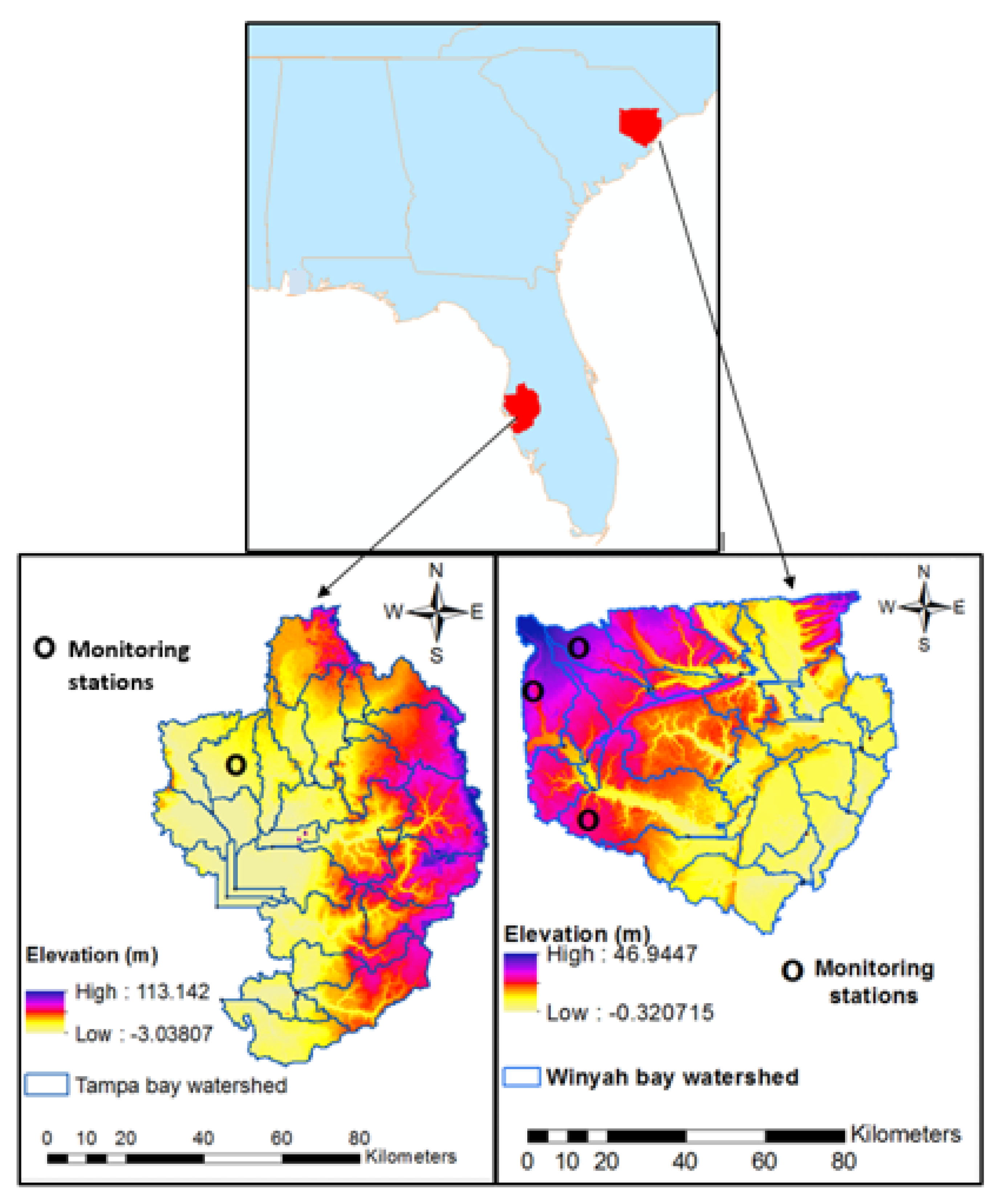
Two case studies were chosen as representations of the water quality constituent of SY evaluated using dynamic soil erodibility and cover management factors with changing space and time. Two basins, the Tampa Bay watershed (TBW) in Florida and the Winyah Bay watershed (WBW) in South Carolina, were used in this study (Figure 2). The TBW is located on the Gulf coast of west-central Florida and has an area of approximately 590,522 km2. The second study area of WBW is approximately 575,590 km2 and encompasses the neighboring areas of the tidal waters of the estuary. The TBW highlights the hydrological responses of a coastal zone with rapid urban development and the WBW highlights the impact of coastal development on increasing soil erosion.
Data and Modeling
The elevation data was rasterized as a 30 m resolution digital elevation model (DEM) from the National Elevation Dataset (NED) provided by the United States Geological Survey (USGS). The soil data concerning texture, depth, and drainage attributes were rasterized from vector maps supplied by the Web Soil Survey (WSS) under the United States Department of Agriculture [80]. The study area watersheds were delineated using the DEMs. The annual land cover maps of the watershed HRUs were developed using a supervised classification analysis based on remotely sensed MODIS images. The developed classifier was trained for the study area watersheds, which produced their supervised classification with fifteen land cover classes [73]. The annually classified land cover maps were employed as the land cover unit in the SWAT model for enhancing hydrological predictions in SWAT.
The models were developed in SWAT for both study areas. A watershed delineation was performed, and several sub-basins were obtained. Then the overlay of land cover, soil, and the slope was carried out, producing the HRUs within the sub-basins. The threshold values used for land cover, soil, and slope while defining the HRUs were 7%, 12%, and 12%, respectively. Later, climate data such as precipitation, temperature, solar radiation, relative humidity, and wind speed were incorporated, model setup was completed, and simulation runs were performed. The stream flows and sediment load from each HRU were calculated separately using input data for weather, soil, topography, vegetation, and land management practices. Later, they were merged to determine the total loadings from the sub-basin as well as from the HRUs. More details and descriptions of the water balance, soil erosion, and water quality process equations can be found in the SWAT technical documentation [72]. Twelve years (2002–2013) of daily weather data were collected from ground weather stations as well as from downscaled and projected data from climate.gov [81,82] with a spatial resolution of 250 m. The observed monthly stream flows and sediment concentrations (Xobserved) obtained from USGS for the years 2002–2013 at the respective monitoring stations were used to calibrate and validate the SWAT model. All the datasets for the study were collected for the years 2002 to 2013 (Table 1). Simulations were done for land cover, soil type, and climate condition of 2002 to 2013 using the weather data with the existing management practices, which generated the simulated stream flows and SY from 2002 to 2013 (Xsimulated). Table 2 and Table 3 explains the descriptive statistics of remotely sensed and modeled soil properties for K-factor estimation in TBW and WBW respectively. The soil texture is stable for a relatively long period of five (2009–2013 in WBW) to eight (2002–2009 in TBW) years in certain parts of the watersheds. However, the majority of the HRUs showcased annual variations in the soil property of AWC, and some of the HRUs showed annual variations for BD and Psoil.
3. Results
3.1. SWAT Calibration and Validation Results
The two case studies were calibrated and validated in varying spatial and temporal conditions. The two different spatial extents (TBW in Florida and WBW in South Carolina) and two different temporal extents (2002–2009 and 2009–2013) were introduced to evaluate the efficacy of SY predictions by the dynamic C and K factors in the SWAT models when there are changes in hydrogeological and spatiotemporal scenarios. The SWAT model was initially set up for the two watersheds in the southeastern United States. TBW was developed with the land cover, soil type, and climate condition for the year 2002 with 29 sub-basins, 2286 HRUs within 29 sub-basins, 15 land cover classes, and 21 soil categories. Similarly, WBW was developed with the land cover, soil type, and climate condition for the year 2009 with 31 sub-basins, 2118 HRUs within 31 sub-basins, 15 land cover classes, and 32 soil categories. The spatial resolution of the HRUs in the study ranged from 9 km to 16 km with an annual temporal resolution. The SWAT model simulations were employed at the levels of seasons, months, and years in the study models. The soil loss predictions were estimated seasonally and monthly in the study watersheds, as opposed to conventional SY predictions on a long-term timespan [83,84,85]. Both the watershed models were calibrated and validated for the years from 2002 to 2013 with the land cover, soil type, and climate conditions for the respective years. The calibration and validation procedure were performed for stream flows as well as SY by selecting the most sensitive parameters affecting stream flows and SY through one-factor-at-a-time sensitivity analysis [86,87]. The most sensitive parameters of ESCO, CN2, and AWCS were used to calibrate stream flows, and ERORGN, ERORGP, and HRU_SLP were used in SY calibration (Table 4).
The study performed three trials each for stream flow and SY calibration, as only six parameters were significantly sensitive to the hydrologic responses of the two basins [87]. AWCS, ESCO, and CN2 were the most critical parameters affecting stream flow patterns in wet conditions because they were found to be highly sensitive to 70% of the stream flows. Even though the parameters such as surface runoff lag coefficient (SURLAG) and Manning’s coefficient for overland flow (OV_N) area are considered to be important in surface flow dynamics, they were obtuse in this study [88,89]. The parameters such as HRU_SLP, ERORGN, ERORGP, average slope length (SLSUBBSN.hru), sediment concentration in lateral and groundwater flow (LAT_SED.hru), and a linear and exponential parameter representing the sediment re-entrained through channel sediment routing (SPCON.bsn, and SPEXP.bsn, respectively) are the conventionally crucial parameters affecting SY [90,91].
However, all the parameters except HRU_SLP, ERORGN, and ERORGP were found to be less sensitive to SY in the study. The methods of auto-calibration (ERORGN and ERORGP) and manual calibration (HRU_SLP) were collectively employed for fast-paced and manageable iterations within the SWAT model. The summary results of calibration and validation are given in Table 5. Overall, for both watersheds, the hydrologic calibration and validation results closely matched the measured values (R2 (0.44–0.85) and NS (0.35–0.75)) for the temporal conditions between 2002 and 2013. The results showed that the model simulations were good estimates in predicting stream flows and SY for Old Tampa Bay, Hillsborough Bay, Middle Tampa Bay, Lower Tampa Bay, and WBW (Figure 3, Table 5).
3.2. Results of Connective Algorithm Validation
The developed K-factor and C-factor and the USLE K-factor and C-factor for the HRUs of the two watersheds were utilized to estimate spatiotemporal SY in the study. The performance results of the statistical evaluation for the implemented model cases are depicted in Table 6. R2, PR2, and NS ranges between 0.5 and 1 are considered to have acceptable goodness of fit in hydrologic modeling purposes [92]. The R2, PR2, and NS values of the generated SY during Case 1 were 0.582, 0.531, and 0.603, respectively, for TBW and 0.503, 0.462, and 0.418, respectively, for WBW. In TBW, they increased to 0.719, 0.636, and 0.741, respectively, after the C-factor data were applied. For the WBW, the increases were 0.594, 0.533, and 0.527, respectively. The dynamic K-factor function (Equation (4)) constitutes the C-factor estimates developed using the remotely sensed variables of EVI, LAI, SR, and AWC (Equation (2)). It designated the repeated implementation of C-factor information in Case 3, where dynamic C-factors and K-factors are connected. PR2 acts as a potent tool to eliminate the overfitting of the model due to the repetition of the C-factor variable [93,94,95]. The increase of PR2 from Case 2 to Case 3 indicated that the twin use of the C-factor variable does not result in overfitting of the SY in Case 3 (TBW: 0.636 (Case 2) to 0.668 (Case 3); WBW: 0.533 (Case 2) to 0.644 (Case 3)).
Figure 4 shows the observed SY versus simulated SY for Cases 1, 2, and 3 at the Rocky Creek monitoring station of TBW and monitoring stations of the Black River, Lynches River, and Pee Dee River in WBW between 2002 and 2013. The significant deviations in actual and simulated SY in Case 1 were significantly reduced in Case 2 during the low SY conditions. This demonstrates that the dynamic C-factor model with the traditional KUSLE model is a better simulator of the low SY that is generally found at the inlet of a watershed and in the dry seasons. Most estimates of lower SY converged to the actual measured values in TBW (NS: 0.603 to 0.741) with the application of the dynamic C-factor and traditional KUSLE, whereas they showed a minor impact in WBW (NS: 0.418 to 0.527). Interestingly, both study areas exhibited potential and further nearness of observed and simulated SY with the connectivity of dynamic K-factor and C-factor (NS: 0.603 to 0.744 (TBW); NS: 0.418 to 0.683 (WBW)). This shows that model efficiency of SY predictions increased for every dynamic factor added; for all cases, the highest model efficiency occurred when the two dynamic factors were connected (Case 3: PR2: 0.60–0.70, R2: 0.70–0.80, NS: 0.65–0.75). These findings emphasized that Case 3 is a much better representation of the actual sediment prediction for different watersheds with varying spatial and temporal environments compared to Case 2. Hence, the connectivity of the dynamic estimates of C-factor and K-factor into SWAT realistically predicted SY when compared to the dynamic assessment using the singular C-factor model [96,97].
The correlations and predictions of Case 3 indicated that the combined application of C-factor and K-factor powerfully represented the SY estimates both for the whole watershed and for the HRUs in the watersheds. This finding is corroborated by some recent studies [98,99]. Despite the different spatial resolution of the various remotely sensed MODIS variables of the study ranging from 30 m to 500 m, the study could demonstrate the advancement of the existing algorithm in predicting the SY. The differences between the actual and estimated SY accounting for the soil erosion for the spatial and temporal extents in the watersheds can be attributed to the modeling techniques, interpolation methods, and real hydrogeological conditions involved in the study areas. These differences also include the ambiguity in the space-wise trends from the IDW technique when interpreting different factors from remote sensing, which were employed in models for catchment scales. Additionally, dynamic modification of the other USLE factors such as rainfall erosion index, support practice factor, and topographic factor might improve the precision and reliability of the spatiotemporal SY estimates in watersheds.
3.3. Spatiotemporal Predictions of C-Factor and K-Factor
The annual C-factors and K-factors for each HRU in the watersheds were calculated using the dynamic functions from Equations (2) and (4) to investigate their distribution in the watersheds. The spatial CUSLE and KUSLE simulated by the SWAT model along with the spatially and temporally dynamic C-factors and K-factors averaged from 2002 to 2009 for TBW and from 2009 to 2013 for WBW are reported in Figure 5. For both watersheds, the C-factor range of 0.01–0.50 was almost 60% of the total watershed, which indicates the dominance of grass and shrubs, pasture, and vegetation in TBW and WBW. The proportion of urban spaces and forests (C-factor: 0–0.01) and wetlands and water (C-factor: 0.5–1) were 35% and 5%, respectively, for TBW and 10% and 30% for WBW. The spatial distribution characteristics of the CUSLE deviated from the annual C-factors averaged from 2002 to 2013. C-factors were found to increase in Lower Tampa Bay, indicating the presence of deforestation as well as land management activities in the Lower Tampa Bay region [22]. The distribution of KUSLE for Lower and Middle TBW was underestimated in comparison with the developed annual K-factors by 45% and 35%, respectively. In contrast, it was overestimated by around 20% and 28% in the northwest and central portions of the WBW, respectively. In both watersheds, no significant annual dynamics were observed in K-factor between 2002 and 2013, despite the noticeable deviation of annual K-factors from the KUSLE.
The K-factor from the USLE equation, KUSLE, considered spatial changes with each HRU while neglecting the temporal dynamics with each year, while the use of the remotely sensed MODIS data estimated accurate soil moisture content. Thus, they captured the spatial as well as annual changes in the developed K-factor function that led to improved K-factor estimation in the watershed. For the years between 2002 and 2009, a K-factor range of 0–0.1 was observed for the Old Tampa Bay and Hillsborough Bay watershed (58% of the total watershed), showing the existence of less erodible soils that can elevate the agricultural productivity encompassing the catchments. Meanwhile, elevated K-factors ranging from 0.1–0.7 were found in the remaining portion of the watershed, which indicates the presence of highly erodible lands and potential risks for soil loss due to erosion. On the other hand, only 20% of the total watershed area showed K-factors between 0–0.1, which leaves a significant portion of the WBW with moderate or highly erodible soils [100,101,102]. Hence it is necessary to adopt sustainable water management measures as well as erosion control strategies within or near the coastal zone for further improvement of agricultural productivity. They will result in coastal water resource improvement [103,104,105].
The trends in the C-factor and K-factor time-series from 2002 to 2013 were determined by computing the C-factors and K-factors averaged annually over all the HRUs of the watershed (Figure 6). The trend analysis results determined a decreasing trend of the watershed C-factors from 2002 to 2013, which confirms the existence of annual management-induced land cover dynamics at the watershed scale [106,107,108,109,110,111]. This highlights the importance of more detailed temporal assessments of crop and cover management for improved investigation of water management in watersheds.
However, on the whole watershed scale, significant increases and sudden decreases were detected in the C-factor time-series from 2003 to 2004 and 2006 to 2007, respectively, in TBW. This result indicates that the C-factor time-series in TBW might not exhibit a consistent pattern for the less dominant land cover distributions. The time-series of K-factors from 2002 to 2013 demonstrated a moderately reducing trend for both watersheds. An evenly transitioning trend was observed in WBW, ranging from 0.218–0.224 in the five years. However, the K-factors in the TBW had minimal changes from 0.206 to 0.210 in the eight years. These findings were substantiated by shreds of research which examined the increasingly important influence that urbanization and its associated soil losses have on the individual drainage basins of TBW and WBW [111]. Thus, the trend test results for the K-factors and C-factors adhere to the real hydrogeological conditions. The inclusion of more precise temporal conditions including seasons, months, days, and hourly intervals holds importance in this context, as these conditions can impact time-series trend detection at the watershed scale, at specific monitoring stations, and concerning point and nonpoint sources of contamination within the watersheds.
4. Discussions
4.1. Spatiotemporal Predictions of Sediment Yields
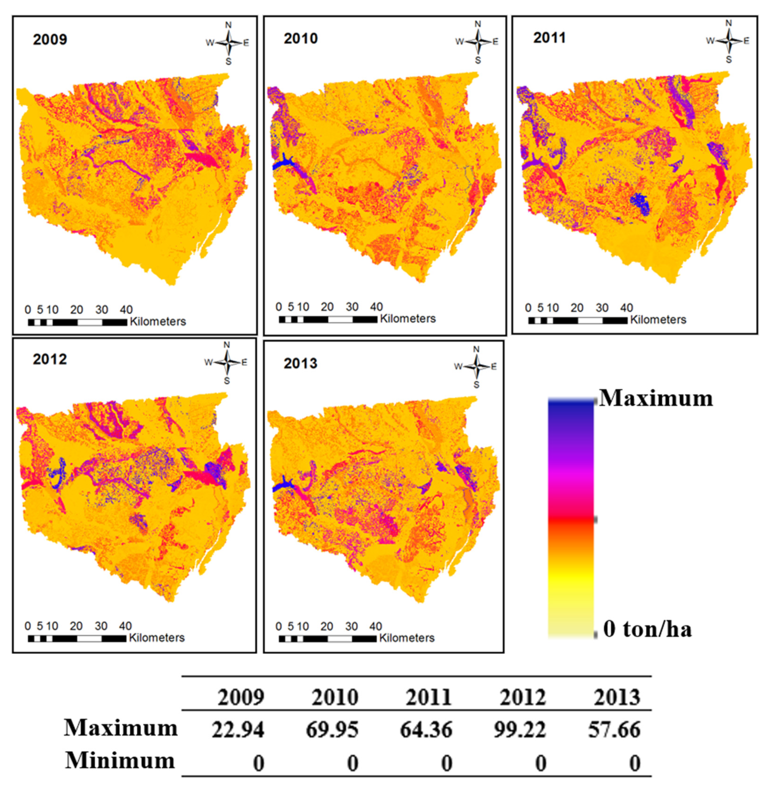
The study illustrated the spatial and temporal variability in SY assessment using a connective algorithm of the dynamic models of the C-factor and K-factor in the SWAT model. Annual SY was generated for each HRU of the watersheds from 2002 to 2013. The annual HRU wise SY ranged from 23 ton/ha to 70 ton/ha. Overall, high sediment deposition was observed in Lower Tampa Bay and Hillsborough Bay, which indicates the accumulation of the collected sediments towards the outlet of the watershed. About 16%, 44%, and 50% of the watershed was associated with the lower, medium, and higher proportions of SY, respectively. However, keen observation was essential to identify the slight reductions in the SY in some parts of Lower Tampa Bay and Old Tampa Bay. This is supported by studies which pointed out significant increases in urban spaces, developed areas, and water cover with corresponding reductions in agricultural productivity [21]. This led to reduced water quality constituents such as suspended sediments and turbidity in TBW. WBW showed moderate yield assessment in which 70%, 22%, and 8% of the watershed was associated with the lower, medium, and higher proportions of SY, respectively. SY was observed to spatially increase from the northwest portion to the southeast portion of the WBW from 2009 to 2013 [112,113]. This shows that with variable spatial resolution (30 m to 500 m) and relatively coarse temporal resolution (annual) satellite remotely sensed data, a good estimate of SY in catchments of the southeastern United States can be made. According to Figure 7 and Figure 8, the spatial variability of sediment generation in the HRUs of both watersheds was much more significant than the temporal variations. Therefore, the temporal variability of the K-factor, which represents the severity of soil and sediment loss, can be neglected when compared to its spatial variation. Some studies support the use of dynamic models for valid water quality assessments in catchments [114,115,116,117,118].
For the year 2007, geospatial changes in the C-factor led to significant reductions in sediment generation in HRUs of TBW. This indicates the improved correlation of the dynamic C-factor and K-factor estimates on water quality predictions compared to the USLE estimates. Hence, they strongly infer the probable association of the connective soil erosional components C-factor and K-factor in changing the water quality of sediments from year to year, especially on watershed scales [119]. Overall, the results showed that the predictions using the developed models are feasible, which can help users to reduce the uncertainty of the quantification of USLE parameters of the C-factor and K-factor.
The vital contribution of the study is the remotely sensed data-driven models proposed, which present a manageable and user-friendly determination of SY for advanced water resource management and can yield advanced spatiotemporal K, C, and SY mapping for watersheds in the United States. In this study, we used K-factor and C-factor to capture the SY dynamics, although these might not fully represent the connectivity of the contributing factors of SY in the areas. Because the catchments have similar areas, mixed land covers, similar soil types, and relative terrain features, we assumed that the whole of the catchments contributed proportionally to the sediment delivered to the outlet [120,121]. However, even in small catchments, SY at the outlet depends on other factors such as atmospheric deposition and groundwater tables, as well as extreme stormwater events. Therefore, a complete understanding of different factors and dynamic SY generation entails the integration of multifaceted environmental and hydrogeological data both at very small scales and at large watershed scales. Furthermore, the annual geospatial maps of C-factors, K-factors, and SY can represent the interannual variability of these factors on SY assessment and soil erosion modeling.
4.2. Study Limitations
The connective framework of the study, which was incorporated in SWAT and tested for the watersheds of the southeastern United States, can be applied to comparable watersheds with mixed land covers. However, extensive spatiotemporal validation of these dynamic models would bolster their global effectiveness in SY predictions and water quality modeling. Regarding the differences between the actual and estimated SY accounting for soil erosion at the spatial and temporal levels in the watersheds, the error is attributable to the lack of alternative dynamic factors, modeling techniques, interpolation methods, and real hydrogeological conditions involved in the study areas. The findings of the study also highlight the necessity of finer spatial and temporal data in real-time water quality modeling of watersheds. Further studies should investigate the connections between unexplored soil erosional factors and water quality, which will broaden knowledge regarding the variability of different water quality constituents and agricultural management in watersheds with changing space and time. Remote sensing-based approaches can be substantially constrained by the coarse resolution of remotely sensed data and the accuracy of its processing, including land cover classification and estimation of various environmental indices. Therefore, justifying a remote sensing-based approach for different study watersheds requires added assessments of how the benefits of the novel models compare to the uncertainties resulting from the fundamental limitations of remote sensing products and methods of their processing, which is outside the scope of this study. In addition, the temporal extents (2002–2009 and 2009–2013), which are much less than 30 years, exert some limitations for long-term studies on soil loss calculations. Nevertheless, the core emphasis of future works should be the elimination of the uncertainties involved in the present study.
5. Conclusions
Various conceptual frameworks of sediment yield assessments have been developed in recent years for enhanced soil erosion modeling. The existing frameworks model singular factors affecting SY; however, they overlook the connection between multiple factors affecting SY spatially and temporally and lack a manageable and user-friendly platform. This study incorporated a new framework of two dynamic factors affecting SY (C-factor and K-factor) into the SWAT model using satellite remotely sensed MODIS data of EVI, SR, AWC, and LAI, and evaluated whether dynamic models can advance spatiotemporal SY predictions in watersheds. We developed a connective algorithm that incorporates all the components required to temporally (annual) and spatially (HRU level) simulate dynamic C-factors and K-factors within the SWAT model. The connective algorithm was validated using sensitivity analysis and three performance indices to determine the impact of the dynamic C-factors and K-factors on SY predictions. The rise in the PR2 (TBW: 0.636 (Case 2) to 0.668 (Case 3); WBW: 0.533 (Case 2) to 0.644 (Case 3)) with the inclusion of the dynamic factors of C and K showed how well the SY was predicted and that the model is not too complicated concerning performance and overfit. The results showed that the model efficiency of SY predictions increased for every dynamic factor added; for all cases, the highest model efficiency occurred when the two dynamic factors were connected (Case 3: PR2: 0.60–0.70, R2: 0.70–0.80, NS: 0.65–0.75). Minor changes in K-factors and gradual decreases in C-factors in the watersheds reflected potential land use changes that can impact sediments and agricultural water use in these regions. The spatiotemporal analysis of the SY simulations generated using the dynamic C-factors and K-factors displayed moderate to high sediment deposition at the watershed outlets. The spatial variability of sediment generation in the HRUs of both watersheds was much more significant than the temporal variations. Therefore, we recommend the application of the dynamic models at smaller spatial scales than the catchment scale to eliminate uncertainty in spatial predictions. Overall, the connective system improved the reliability of SY predictions in SWAT and created options for applying remotely sensed data unlike the conventional USLE functions existing in SWAT.
The study concluded that satellite remotely sensed data of EVI, SR, LAI, and AWC can effectively be used in spatiotemporal estimation of the dynamic C-factor and K-factor, as well as SY, within basin-scale hydrologic models. The results emphasized the greater feasibility of SY and water demand predictions in SWAT when all the satellite remotely sensed dynamic variables are implemented in the connective algorithm of the C-factor and K-factor. This can help users to reduce the uncertainty of the quantification of USLE parameters of the C-factor and K-factor with the aid of the SWAT model. The vital contribution of the study is the remotely sensed data-driven models proposed that put forth a manageable and user-friendly determination of SY and can yield advanced spatiotemporal K, C, and SY mapping for watersheds in the United States. Regarding the differences between the actual and estimated SY accounting for the soil erosion for the spatial and temporal extents in the watersheds, the error is attributable to the modeling techniques, interpolation methods, and real hydrogeological conditions involved in the study areas. The findings of the study highlight the necessity of better spatial and temporal data in real-time water quality modeling of watersheds in order to ensure hydro-environmental health. Further studies should investigate the underlying uncertainties of remote sensing-based approaches as well as the relationships between unexplored soil erosional factors and water quality in watersheds with changing space and time.
Author Contributions
Conceptualization, P.P.; methodology, P.P.; software, P.P.; validation, P.P. and A.A.-H.; formal analysis, P.P.; investigation, A.A.-H.; resources, A.A.-H.; data curation, P.P.; writing—original draft preparation, P.P.; writing—review and editing, P.P. and A.A.-H.; visualization, P.P.; supervision, A.A.-H.; project administration, A.A.-H.; funding acquisition, A.A.-H. All authors have read and agreed to the published version of the manuscript.
Funding
This research received no external funding.
Data Availability Statement
Data will be available upon request.
Acknowledgments
I would like to acknowledge the reviewers for enhancing the article.
Conflicts of Interest
The authors declare no conflict of interest.
References
- Lal, R. Soil degradation by erosion. Land Degrad. Dev. 2001, 12, 519–539. [Google Scholar] [CrossRef]
- Montanarella, L. Trends in Land Degradation in Europe; Springer: Berlin, Germany, 2007; pp. 83–104. Available online: http://www.wamis.org/agm/meetings/wocald06/S2-Montanarella.pdf (accessed on 25 January 2020).
- Young, C.J.; Liu, S.; Schumacher, J.A.; Schumacher, T.E.; Kaspar, T.C.; McCarty, G.W.; Napton, D.; Jaynes, D.B. Evaluation of a model framework to estimate soil and soil organic carbon redistribution by water and tillage using 137Cs in two US Midwest agricultural fields. Geoderma 2014, 232, 437–448. [Google Scholar] [CrossRef]
- Kinnell, P.I.A. Determining soil erodibilities for the USLEMM rainfall erosion model. Catena 2018, 163, 424–426. [Google Scholar] [CrossRef]
- Bernatek-Jakiel, A.; Poesen, J. Subsurface erosion by soil piping: Significance and research needs. Earth Sci. Rev. 2018, 185, 1107–1128. [Google Scholar] [CrossRef]
- Preetha, P.P.; Al-Hamdan, A.Z.; Anderson, M.D. Assessment of climate variability and short term land use land cover change effects on water quality of Cahaba river basin. Int. J. Hydrol. Sci. Technol. 2019, 11, 54–75. [Google Scholar] [CrossRef]
- Preetha, P.P.; Al-Hamdan, A.Z. Developing Nitrate-Nitrogen Transport Models using Remotely-Sensed Geospatial Data of Soil Moisture Profiles and Wet Depositions. J. Environ. Sci. Health Part A 2020, 55, 615–628. [Google Scholar] [CrossRef]
- Kwon, H.; Park, G.; Kim, S. Estimation of soil loss changes and sediment transport path using GIS and multi-temporal RS data. J. GIS Assoc. Korea 2002, 10, 134–147. [Google Scholar] [CrossRef] [Green Version]
- Cho, H.L.; Jeong, J.C. Estimating soil loss in alpine farmland with RUSLE and SEDD. J. GIS Assoc. Korea 2005, 13, 79–90. [Google Scholar]
- Lee, G.; Hwang, E. The influence analysis of GIS-based soil Erosion in water-pollutant buffering zone. J. Korean Soc. Civ. Eng. 2006, 26, 335–340. [Google Scholar]
- Wischmeier, W.H.; Smith, D.D. Predicting rainfall-erosion losses—A guide to conservation planning. In Agriculture Handbook 537; US Department of Agriculture: Washington, DC, USA, 1978. Available online: https://naldc.nal.usda.gov/download/CAT79706928/PDF (accessed on 17 January 2019).
- Renard, K.G.; Foster, G.R.; Weesies, G.A.; McCool, D.K. Predicting Soil Erosion by Water: A Guide to Conservation Planning with the Revised Universal Soil Loss Equation (RUSLE); Agricultural Handbook; US Department of Agriculture: Washington, DC, USA, 1997; Volume 703. Available online: https://www3.epa.gov/npdes/pubs/ruslech2.pdf (accessed on 17 January 2019).
- Renard, K.G.; Foster, G.R.; Weesies, G.A. RUSLE: Revised universal soil loss equation. J. Soil Water Conserv. 1991, 46, 30–33. [Google Scholar]
- Williams, J.R. Sediment routing for agricultural watersheds. JAWRA 1975, 11, 965–974. [Google Scholar] [CrossRef]
- Kinnell, P.I.A.; Risse, L.M. USLE-M: Empirical modeling rainfall erosion through runoff and sediment concentration. Soil Sci. Soc. Am. J. 1998, 62, 1667–1672. [Google Scholar] [CrossRef]
- Flacke, W.; Auerswald, K.; Neufang, L. Combining a modified Universal Soil Loss Equation with a digital terrain model for computing high resolution maps of soil loss resulting from rain wash. Catena 1990, 17, 383–397. [Google Scholar] [CrossRef]
- Van Oost, K.; Govers, G.; Desmet, P. Evaluating the effects of changes in landscape structure on soil erosion by water and tillage. Landsc. Ecol. 2000, 15, 577–589. [Google Scholar] [CrossRef]
- Van Rompaey, A.J.; Verstraeten, G.; Van Oost, K.; Govers, G.; Poesen, J. Modelling mean annual sediment yield using a distributed approach. Earth Surf. Process. Landf. 2001, 26, 1221–1236. [Google Scholar] [CrossRef]
- Haregeweyn, N.; Yohannes, F. Testing and evaluation of the agricultural non-point source pollution model (AGNPS) on Augucho catchment, western Hararghe, Ethiopia. Agric. Ecosyst. Environ. 2003, 99, 201–212. [Google Scholar] [CrossRef]
- Xian, G.; Crane, M. Assessments of urban growth in the TBW using remote sensing data. Remote Sens. Environ. 2005, 97, 203–215. [Google Scholar] [CrossRef]
- Moreno-Madrinan, M.J.; Al-Hamdan, M.Z.; Rickman, D.L.; Muller-Karger, F.E. Using the surface reflectance MODIS Terra product to estimate turbidity in Tampa Bay, Florida. Remote Sens. 2010, 2, 2713–2728. [Google Scholar] [CrossRef]
- Moreno-Madrinan, M.J.M.; Al-Hamdan, M.Z.; Rickman, D.L.; Ye, J. Relationship between watershed land cover/land-use change and water turbidity status of Tampa Bay major tributaries, Florida, USA. Water Air Soil Pollut. 2012, 223, 2093–2109. [Google Scholar] [CrossRef]
- Pandey, A.; Himanshu, S.K.; Mishra, S.; Singh, V.P. Physically based soil erosion and sediment yield models revisited. Catena 2016, 147, 595–620. [Google Scholar] [CrossRef]
- Prasannakumar, V.; Vijith, H.; Abinod, S.; Geetha, N. Estimation of soil erosion risk within a small mountainous sub-watershed in Kerala, India, using Revised Universal Soil Loss Equation (RUSLE) and geo-information technology. Geosci. Front. 2012, 3, 209–215. [Google Scholar] [CrossRef] [Green Version]
- Mancino, G.; Nole, A.; Ripullone, F.; Ferrara, A. Landsat TM imagery and NDVI differencing to detect vegetation change: Assessing natural forest expansion in Basilicata, southern Italy. iForest 2014, 7, 75–84. [Google Scholar] [CrossRef] [Green Version]
- Karaburun, A. Estimation of C-factor for soil erosion modeling using NDVI in Buyukcekmece watershed. OJAS Ozean J. Appl. Sci. 2010, 3, 77–85. [Google Scholar]
- Waldhoff, G.; Lussem, U.; Bareth, G. Multi-data approach for remote sensing-based regional crop rotation mapping: A case study for the Rur catchment, Germany. Int. J. Appl. Earth Obs. 2017, 61, 55–69. [Google Scholar] [CrossRef]
- De Jong, S.M.; Paracchini, M.L.; Bertolo, F.; Folving, S.; Megier, J.; De Roo, A.P.J. Regional assessment of soil erosion using the distributed model SEMMED and remotely-sensed data. Catena 1999, 37, 291–308. [Google Scholar] [CrossRef]
- Gertner, G.; Wang, G.; Fang, S.; Anderson, A.B. Mapping and uncertainty of predictions based on multiple primary variables from joint co-simulation with Landsat TM image and polynomial regression. Remote Sens. Environ. 2002, 83, 498–510. [Google Scholar] [CrossRef]
- Yuan, F. Land-cover change and environmental impact analysis in the Greater Mankato area of Minnesota using remote sensing and GIS modeling. Int. J. Remote Sens. 2008, 29, 1169–1184. [Google Scholar] [CrossRef]
- Godínez-Alvarez, H.; Herrick, J.E.; Mattocks, M.; Toledo, D.; Van Zee, J. Comparison of three vegetation monitoring methods: Their relative utility for ecological assessment and monitoring. Ecol. Indic. 2009, 9, 1001–1008. [Google Scholar] [CrossRef]
- Bieger, K.; Arnold, J.G.; Rathjens, H.; White, M.J.; Bosch, D.D.; Allen, P.M.; Srinivasan, R. Introduction to SWAT+, a completely restructured version of the soil and water assessment tool. JAWRA J. Am. Water Resour. Assoc. 2016, 53, 115–130. [Google Scholar] [CrossRef]
- Folly, A.; Bronsveld, M.C.; Clavaux, M. A knowledge-based approach for C-factor mapping in Spain using Landsat TM and GIS. Int. J. Remote Sens. 1996, 17, 2401–2415. [Google Scholar] [CrossRef]
- Wang, G.; Wente, S.; Gertner, G.Z.; Anderson, A. Improvement in mapping vegetation cover factor for the universal soil loss equation by geostatistical methods with Landsat Thematic Mapper images. Int. J. Remote Sens. 2002, 23, 3649–3667. [Google Scholar] [CrossRef]
- Matsushita, B.; Yang, W.; Chen, J.; Ond, Y.; Qiu, G. Sensitivity of the Enhanced Vegetation Index (EVI) and Normalized Difference Vegetation Index (NDVI) to topographic effects: A case study in high-density Cypress forest. Sensors 2007, 7, 2636–2651. [Google Scholar] [CrossRef] [PubMed] [Green Version]
- Panico, S.C.; Memoli, V.; Esposito, F.; Maisto, G.; De Marco, A. Plant cover and management practices as drivers of soil quality. Appl. Soil Ecol. 2018, 129, 34–42. [Google Scholar] [CrossRef]
- McDonald, S.E.; Reid, N.; Waters, C.M.; Smith, R.; Hunter, J. Improving ground cover and landscape function in a semi-arid rangeland through alternative grazing management. Agric. Ecosyst. Environ. 2018, 268, 8–14. [Google Scholar] [CrossRef]
- Foster, G.R. Draft: Science Documentation, Revised Universal Soil Loss Equation Version 2 (RUSLE2); USDA—Agricultural Research Service: Washington, DC, USA, 2005. [Google Scholar]
- Zhang, K.L.; Shu, A.P.; Xu, X.L.; Yang, Q.K.; Yu, B. Soil erodibility and its estimation for agricultural soils in China. J. Arid Environ. 2008, 72, 1002–1011. [Google Scholar] [CrossRef]
- Vaezi, A.R.; Sadeghi, S.H.; Bahrami, H.A.; Mahdian, M. Modeling the USLE K-factor for calcareous soils in northwestern Iran. Geomorphology 2008, 97, 414–423. [Google Scholar] [CrossRef]
- Mattheus, C.; Norton, M. Comparison of pond-sedimentation data with a GIS-based USLE model of sediment yield for a small forested urban watershed. Anthropocene 2013, 2, 89–101. [Google Scholar] [CrossRef]
- Shabani, F.; Kumar, L.; Esmaeili, A. Improvement to the prediction of the USLE K factor. Geomorphology 2014, 204, 229–234. [Google Scholar] [CrossRef]
- Ostovari, Y.; Ghorbani-Dashtaki, S.; Bahrami, H.; Naderi, M.; Dematte, J.; Kerry, R. Modification of the USLE k factor for soil erodibility assessment on calcareous soils in Iran. Geomorphology 2016, 273, 385–395. [Google Scholar] [CrossRef]
- Wang, B.; Zheng, F.; Guan, Y. Improved USLE-k factor prediction: A case study on water erosion areas in China. Int. Soil Water Conserv. Res. 2016, 4, 168–176. [Google Scholar] [CrossRef] [Green Version]
- Molina-Navarro, E.; Andersen, H.; Nielsen, A.; Thodsen, H.; Trolle, D. The impact of the objective function in multi-site and multi-variable calibration of the SWAT model. Environ. Model Softw. 2017, 93, 255–267. [Google Scholar] [CrossRef]
- Pham, T.G.; Degener, J.; Kappas, M. Integrated universal soil loss equation (USLE) and geographical information system (GIS) for soil erosion estimation in a sap basin; Central Vietnam. Int. Soil Water Conserv. Res. 2018, 6, 99–110. [Google Scholar] [CrossRef]
- Basic, F.; Kisic, I.; Mesic, M.; Nestroy, O.; Butorac, A. Tillage and crop management effects on soil erosion in central Croatia. Soil Tillage Res. 2004, 78, 197–206. [Google Scholar] [CrossRef]
- Ucar, Z.; Bettinger, P.; Merry, K.; Akbulut, R.; Siry, J. Estimation of urban woody vegetation cover using multispectral imagery and LiDAR. Urban For. Urban Green. 2018, 29, 248–260. [Google Scholar] [CrossRef]
- Deng, J.S.; Wang, K.; Deng, Y.H.; Qi, G.J. PCA-based land-use change detection and analysis using multitemporal and multisensor satellite data. Int. J. Remote Sens. 2008, 29, 4823–4838. [Google Scholar] [CrossRef]
- Wu, H.; Chen, B. Evaluating uncertainty estimates in distributed hydrological modeling for the Wenjing River watershed in China by GLUE, SUFI-2, and ParaSol methods. Ecol. Eng. 2015, 76, 110–121. [Google Scholar] [CrossRef]
- Abbaspour, K.C.; Johnson, C.A.; van Genuchten, M.T. Estimating uncertain flow and transport parameters using a sequential uncertainty fitting procedure. Vadose Zone J. 2004, 3, 1340–1352. [Google Scholar] [CrossRef]
- Abbaspour, K.C.; Rouholahnejad, E.; Vaghefi, S.; Srinivasan, R.; Yang, H.; Kløve, B. A continental-scale hydrology and water quality model for Europe: Calibration and uncertainty of a high-resolution large-scale SWAT model. J. Hydrol. 2015, 524, 733–752. [Google Scholar] [CrossRef] [Green Version]
- Wellen, C.; Arhonditsis, G.B.; Long, T.; Boyd, D. Quantifying the uncertainty of nonpoint source attribution in distributed water quality models: A Bayesian assessment of SWAT’s sediment export predictions. J. Hydrol. 2014, 519, 3353–3368. [Google Scholar] [CrossRef]
- Santhi, C.; Arnold, J.G.; Williams, J.R.; Dugas, W.A.; Srinivasan, R.; Hauck, L.M. Validation of the SWAT model on a large river basin with point and nonpoint sources. J. Am. Water Resour. Assoc. 2001, 37, 1169–1188. [Google Scholar] [CrossRef]
- Van Griensven, A.; Ndomba, P.; Yalew, S.; Kilonzo, F. Critical review of SWAT applications in the upper Nile basin countries. Hydrol. Earth Syst. Sci. 2012, 16, 3371–3381. [Google Scholar] [CrossRef] [Green Version]
- Zeiger, S.J.; Hubbart, J.A. A SWAT model validation of nested-scale contemporaneous stream flow, suspended sediment and nutrients from a multiple-land-use watershed of the central USA. Sci. Total Environ. 2016, 572, 232–243. [Google Scholar] [CrossRef] [PubMed]
- Arnold, J.; Bieger, K.; White, M.; Srinivasan, R.; Dunbar, J.; Allen, P. Use of Decision Tables to Simulate Management in SWAT+. Water 2018, 10, 713. [Google Scholar] [CrossRef] [Green Version]
- Li, R.; Li, J. Satellite remote sensing technology for lake water clarity monitoring: An overview. Environ. Inf. Arch. 2004, 2, 893–901. [Google Scholar]
- Schultz, G.A.; Engman, E.T. Remote Sensing in Hydrology and Water Management; Springer: Berlin/Heidelberg, Germany, 2000. [Google Scholar]
- Chen, Z.; Hu, C.; Muller-Karger, F. Monitoring turbidity in Tampa Bay using MODID/Aqua 250-m imagery. Remote Sens. Environ. 2007, 109, 207–220. [Google Scholar] [CrossRef]
- USGS LP DAAC. MODIS/Terra Surface Reflectance 8-Day L3 Global 500m SIN Grid V006. 2019. Available online: https://search.earthdata.nasa.gov/search/granules?p=C193529899-LPDAAC_ECS&tl=1534089058!4!!&q=modis%20surface&ok=modis%20surface (accessed on 23 January 2019).
- Hajigholizadeh, M. Water Quality Modelling Using Multivariate Statistical Analysis and Remote Sensing in South Florida. Ph.D. Thesis, Florida International University, Miami, FL, USA, 2016. [Google Scholar]
- Weng, Q. Land use change analysis in the Zhujiang delta of China using satellite remote sensing, GIS and stochastic modeling. J. Environ. Econ. Manag. 2002, 64, 273–284. [Google Scholar] [CrossRef] [Green Version]
- Wu, Q.; Li, H.; Wang, R.; Paulussen, J.; He, Y.; Wang, M.; Wang, B.; Wang, Z. Monitoring and predicting land use change in Beijing using remote sensing and GIS. Landsc. Urban Plan. 2006, 78, 322–333. [Google Scholar] [CrossRef]
- Onate-Valdivieso, F.; Sendra, J.B. Application of GIS and remote sensing techniques in generation of land use scenarios for hydrological modeling. J. Hydrol. 2010, 395, 256–263. [Google Scholar] [CrossRef]
- Li, L.; Meng, Q.Y. Reviews of phosphorus transport and transformation in soil under freezing and thawing actions. Front. Ecol. Environ. 2013, 6, 1074–1078. [Google Scholar]
- Asmamaw, L.B.; Mohammed, A.A. Effects of slope gradient and changes in land use/cover on selected soil physico-biochemical properties of the Gerado catchment, north-eastern Ethiopia. Int. J. Environ. Stud. 2013, 70, 111–125. [Google Scholar] [CrossRef]
- Mugagga, F.; Kakembo, V.; Buyinza, M. Land use changes on the slopes of Mount Elgon and the implications for the occurrence of landslides. Catena 2012, 90, 39–46. [Google Scholar] [CrossRef]
- USGS. LP DAAC. MODIS/Terra Leaf Area Index/FPAR 8-Day L4 Global 500m SIN Grid V006. 2019. Available online: https://search.earthdata.nasa.gov/search/granules?p=C203669720-LPDAAC_ECS&tl=1534089058!4!!&q=modis%20lai&ok=modis%20lai (accessed on 17 January 2019).
- USGS. LP DAAC. MODIS/Terra Vegetation Indices 16-Day L3 Global 250m SIN Grid V006. 2019. Available online: https://search.earthdata.nasa.gov/search/granules?p=C194001241-LPDAAC_ECS&tl=1534089058!4!!&q=modis%20evi&ok=modis%20evi (accessed on 25 January 2019).
- Preetha, P.P.; Al-Hamdan, A.Z. Synergy of remotely sensed data in spatiotemporal dynamic modeling of the crop and cover management factor. Pedosphere 2022, 32, 381–392. [Google Scholar] [CrossRef]
- Neitsch, S.L.; Arnold, J.G.; Kiniry, J.R.; Williams, J.R. Soil & Water Assessment Tool: Theoretical Documentation Version 2009; TR-406; Texas Water Resources Institute: Temple, TX, USA, 2011; Available online: https://swat.tamu.edu/media/99192/swat2009-theory.pdf (accessed on 24 January 2020).
- Preetha, P.P.; Al-Hamdan, A.Z. Multi-level pedotransfer modification functions of the USLE-K factor for annual soil erodibility estimation of mixed landscapes. Model. Earth Syst. Environ. 2019, 5, 767–779. [Google Scholar] [CrossRef]
- Arnold, J.G.; Srinivasan, R.; Muttiah, R.S.; Williams, J.R. Large area hydrologic modeling and assessment Part I: Model development. JAWRA J. Am. Water Resour. Assoc. 1998, 34, 73–89. [Google Scholar] [CrossRef]
- Neitsch, S.L.; Arnold, J.G.; Kiniry, J.R.; Williams, J.R. Soil and Water Assessment Tool Theoretical Documentation Version 2000: Draft-April 2001; Grassland, Soil and Water Research Laboratory: Temple, TX, USA, 2001. [Google Scholar]
- Risal, A. Application of Web ERosivity Module (WERM) for estimation of annual and monthly R factor in Korea. Catena 2016, 147, 225–237. [Google Scholar] [CrossRef]
- Sadeghi, S.H.; Zabihi, M.; Vafakhah, M.; Hazbavi, Z. Spatiotemporal mapping of rainfall erosivity index for different return periods in Iran. Nat. Hazards 2017, 87, 35–56. [Google Scholar] [CrossRef]
- Yue, S.; Wang, C. The Mann-Kendall test modified by effective sample size to detect trend in serially correlated hydrological series. Water Resour. Manag. 2004, 18, 201–218. [Google Scholar] [CrossRef]
- Onoz, B.; Bayazit, M. Block bootstrap for Mann–Kendall trend test of serially dependent data. Hydrol. Process. 2012, 26, 3552–3560. [Google Scholar] [CrossRef]
- USDA. Description of U.S. General Soil Map (STATSGO2). Web Soil Survey. 2018. Available online: https://websoilsurvey.sc.egov.usda.gov/App/WebSoilSurvey.aspx (accessed on 10 January 2019).
- Neitsch, S.L.; Arnold, J.G.; Kiniry, J.R.; Williams, J.R. Soil and Water Assessment Tool (SWAT) Theoretical Documentation; TR-406; Blackland Research Center, Grassland, Soil and Water Research Laboratory, Agricultural Research Service: Temple, TX, USA, 2005. [Google Scholar]
- NOAA. Average Temperature: Stabilized Emissions, Projections. Climate.gov. 2017. Available online: https://www.climate.gov/maps-data/data-snapshots/averagemaxtemp-decade-LOCA-rcp85-2090-02-00?theme=Projections (accessed on 4 October 2017).
- Xu, Z.X.; Pang, J.P.; Liu, C.M.; Li, J.Y. Assessment of runoff and sediment yield in the miyun reservoir catchment by using swat model. Hydrol. Process. 2009, 23, 3619–3630. [Google Scholar] [CrossRef]
- Zhang, A.; Zhang, C.; Fu, G.; Wang, B.; Bao, Z.; Zheng, H. Assessments of impacts of climate change and human activities on runoff with swat for the huifa river basin, northeast china. Water Resour. Manag. 2012, 26, 2199–2217. [Google Scholar] [CrossRef]
- Swami, V.; Kulkarni, S. Simulation of runoff and sediment yield for a Kaneri watershed using SWAT model. J. Geosci. Environ. Prot. 2016, 4, 62200. [Google Scholar] [CrossRef] [Green Version]
- Moriasi, D.N.; Wilson, B.N.; Douglas-Mankin, K.R.; Arnold, J.G.; Gowda, P.H. Hydrologic and water quality models: Use, calibration, and validation. Trans. ASABE 2012, 55, 1241–1247. [Google Scholar] [CrossRef]
- Yesuf, H.; Assen, M.; Alamirew, T.; Melesse, A. Modeling of sediment yield in Maybar gauged watershed using SWAT, northeast Ethiopia. Catena 2015, 127, 191–205. [Google Scholar] [CrossRef]
- Worqlul, A.W.; Ayana, E.K.; Yen, H.; Jeong, J.; MacAlister, C.; Taylor, R.; Gerik, T.J.; Steenhuis, T.S. Evaluating hydrologic responses to soil characteristics using SWAT model in a paired-watersheds in the Upper Blue Nile basin. Catena 2018, 163, 332–341. [Google Scholar] [CrossRef]
- Thapa, B.R.; Ishidaira, H.; Pandey, V.P.; Shakya, N.M. A multi-model approach for analyzing water balance dynamics in Kathmandu Valley, Nepal. J. Hydrol. Reg. Stud. 2017, 9, 149–162. [Google Scholar] [CrossRef]
- Saraswat, D.; Youssef, M.A. A recommended calibration and validation strategy for hydrologic and water quality models. Trans. ASABE 2015, 58, 1705–1719. [Google Scholar] [CrossRef] [Green Version]
- Asadzadeh, M.; Leon, L.; Yang, W.; Bosch, D. One-day offset in daily hydrologic modeling: An exploration of the issue in automatic model calibration. J. Hydrol. 2016, 534, 164–177. [Google Scholar] [CrossRef]
- Akhavan, M.; Imhoff, P.T.; Andres, A.S.; Finsterle, S. Model evaluation of denitrification under rapid infiltration 636 basin systems. J. Contam. Hydrol. 2013, 152, 18–34. [Google Scholar] [CrossRef] [PubMed]
- Veall, M.R.; Zimmermann, K.F. Pseudo-R2 measures for some common limited dependent variable models. J. Econ. Surv. 1996, 10, 241–259. [Google Scholar] [CrossRef] [Green Version]
- Roy, K.; Leonard, J.T. On selection of training and test sets for the development of predictive QSAR models. QSAR Comb. Sci. 2006, 25, 235–251. [Google Scholar]
- Schuurmann, G.; Ebert, R.U.; Chen, J.; Wang, B.; Kuhne, R. External validation and prediction employing the predictive squared correlation coefficient test set activity mean vs. training set activity mean. J. Chem. Inf. Model. 2008, 48, 2140–2145. [Google Scholar] [CrossRef] [PubMed]
- Mahmoodabadi, M. Sediment yield estimation using a semi-quantitative model and GIS-remote sensing data. Int. Agrophys. 2011, 25, 241–247. [Google Scholar]
- Vemu, S.; Pinnamaneni, U.B. Sediment yield estimation and prioritization of watershed using remote sensing and GIS. Int. Arch. Photogramm. Remote Sens. Spat. Inf. Sci. 2012, XXXIX-B8, 529–533. [Google Scholar] [CrossRef] [Green Version]
- Anache, J.A.A.; Bacchi, C.G.V.; Panachuki, E.; Sobrinho, T.A. Assessment of Methods for Predicting Soil Erodibility in Soil Loss Modeling. Geociências São Paulo 2016, 34, 32–40. [Google Scholar]
- Almagro, A.; Thomé, T.C.; Colman, C.B.; Pereira, R.B.; Marcato Junior, J.; Rodrigues, D.B.B.; Oliveira, P.T.S. Improving cover and management factor (C-factor) estimation using remote sensing approaches for tropical regions. Int. Soil Water Conserv. Res. 2019, 7, 325–334. [Google Scholar] [CrossRef]
- Alegria, H.A.; Shaw, T.J. Rain deposition of pesticides in coastal waters of the South Atlantic bight. Environ. Sci. Technol. 1999, 33, 850–856. [Google Scholar] [CrossRef]
- Patchineelam, S.M.; Kjerfve, B.; Gardner, L.R. A preliminary sediment budget for the Winyah Bay estuary, South Carolina, USA. Mar. Geol. 1999, 162, 133–144. [Google Scholar] [CrossRef]
- Gardner, L.R.; Kjerfv, B. Tidal fluxes of nutrients and suspended sediments at the North Inlet—Winyah Bay National Estuarine Research Reserve. Estuar. Coast. Shelf Sci. 2006, 70, 682–692. [Google Scholar] [CrossRef]
- Martins, S.G.; Silva, M.L.N.; Avanzi, J.C.; Curi, N.; Fonseca, S. Cover-management factor and soil and water losses from eucalyptus cultivation and Atlantic Forest at the Coastal Plain in the Espírito Santo State, Brazil. Sci. For. 2010, 38, 517–526. [Google Scholar]
- Oliveira, P.T.S.; Nearing, M.A.; Wendland, E. Orders of magnitude increase in soil erosion associated with land use change from native to cultivated vegetation in a Brazilian savannah environment. Earth Surf. Process. Landf. 2015, 40, 1524–1532. [Google Scholar] [CrossRef]
- Alewell, C.; Borrelli, P.; Meusburger, K.; Panagos, P. Using the USLE: Chances, challenges and limitations of soil erosion modelling. Int. Soil Water Conserv. Res. 2019, 7, 203–225. [Google Scholar] [CrossRef]
- Kucklick, J.R.; Sivertsen, S.K.; Sanders, M.; Scott, G.L. Factors influencing polycyclic aromatic hydrocarbon distributions in South Carolina estuarine sediments. J. Exp. Mar. Biol. Ecol. 1997, 213, 13–29. [Google Scholar] [CrossRef]
- Lo, C.P.; Yang, X. Drivers of land-use/land-cover changes and dynamic modeling for the Atlanta, Georgia metropolitan area. Photogramm. Eng. Remote Sens. 2002, 68, 1073–1082. [Google Scholar]
- Loveland, T.R.; Sohl, T.L.; Stehman, S.V.; Gallant, A.L.; Sayler, K.L.; Napton, D.E. A strategy for estimating the rates of recent United States land-cover changes. Photogramm. Eng. Remote Sens. 2002, 68, 1091–1099. [Google Scholar]
- Arnfield, A.J. Two decades of urban climate research: A review of turbulence, exchanges of energy and water, and the urban heat island. Int. J. Climatol. 2003, 23, 1–26. [Google Scholar] [CrossRef]
- Gillies, R.R.; Box, J.B.; Symanzik, J.; Rodemaker, E.J. Effects of urbanization on the aquatic fauna of the Line Creek watershed, Atlanta—A satellite perspective. Remote Sens. Environ. 2003, 86, 411–422. [Google Scholar] [CrossRef] [Green Version]
- Lawrenz, E.; Pinckney, J.L.; Ranhofer, M.L.; MacIntyre, H.L.; Richardson, T.L. Spectral irradiance and phytoplankton community composition in a blackwater-dominated estuary, Winyah Bay, South Carolina, USA. Estuaries Coast. 2010, 33, 1186–1201. [Google Scholar] [CrossRef]
- Hutchinson, S.E.; Sklar, F.H.; Roberts, C. Short term sediment dynamics in a Southeastern U.S.A. spartina marsh. J. Coast. Res. 1995, 11, 370–380. [Google Scholar]
- Patchineelam, S.M.; Kjerfve, B. Suspended sediment variability on seasonal and tidal time scales in the Winyah Bay estuary, South Carolina, USA. Estuar. Coast. Shelf Sci. 2004, 59, 307–318. [Google Scholar] [CrossRef]
- Zhang, L.; O’Neill, A.L.; Lacey, S. Modelling approaches to the prediction of soil erosion in catchments. Environ. Softw. 1996, 11, 123–133. [Google Scholar] [CrossRef]
- Torri, D.; Poesen, J.; Borselli, L. Predictability and uncertainty of the soil erodibility factor using a global dataset. Catena 1997, 31, 1–22. [Google Scholar] [CrossRef]
- Moriasi, D.N.; Arnold, J.G.; Van Liew, M.W.; Bingner, R.L.; Harmel, R.D.; Veith, T.L. Model evaluation guidelines for systematic quantification of accuracy in watershed simulations. Trans. ASABE 2007, 50, 885–900. [Google Scholar] [CrossRef]
- Hsiao, C.Y.; Lin, B.S.; Chen, C.K.; Chang, D.W. Application of airborne LiDAR technology in analyzing sediment-related disasters and effectiveness of conservation management in Shihmen Watershed. J. GeoEng. 2014, 9, 55–73. [Google Scholar]
- Lin, B.S.; Thomas, K.; Chen, C.K.; Ho, H.C. Evaluation of Soil Erosion Risk for Watershed Management in Shenmu Watershed, Central Taiwan Using USLE Model Parameters, Central Taiwan. Paddy Water Environ. 2016, 14, 19–43. [Google Scholar] [CrossRef]
- Liu, Y.H.; Li, D.H.; Chen, W.; Lin, B.S.; Seeboonruang, U.; Tsai, F. Soil erosion modeling and comparison using slope units and grid cells in Shihmen reservoir watershed in northern Taiwan. Water 2018, 10, 1387. [Google Scholar] [CrossRef] [Green Version]
- Parsons, A.J.; Brazier, R.E.; Wainwright, J.; Powell, D.M. Scale relationships in hillslope runoff and erosion. Earth Surf. Process. Landf. 2006, 31, 1384–1393. [Google Scholar] [CrossRef]
- Parsons, A.J.; Bracken, L.; Poeppl, R.E.; Wainwright, J.; Keesstra, S.D. Introduction to special issue on connectivity in water and sediment dynamics. Earth Surf. Process. Landf. 2015, 40, 1275–1277. [Google Scholar] [CrossRef] [Green Version]
Figure 1.
The workflow of the proposed algorithm for obtaining dynamic C-factor, K-factor, and SY.

Figure 2.
Location of the study areas of TBW and WBW with the employed monitoring stations.

Figure 3.
The observed versus simulated stream flows in the calibration and validation for (a) TBW (n = 89) and (b) WBW (n = 139). n is the number of data points used for calibration and validation.
Figure 3.
The observed versus simulated stream flows in the calibration and validation for (a) TBW (n = 89) and (b) WBW (n = 139). n is the number of data points used for calibration and validation.
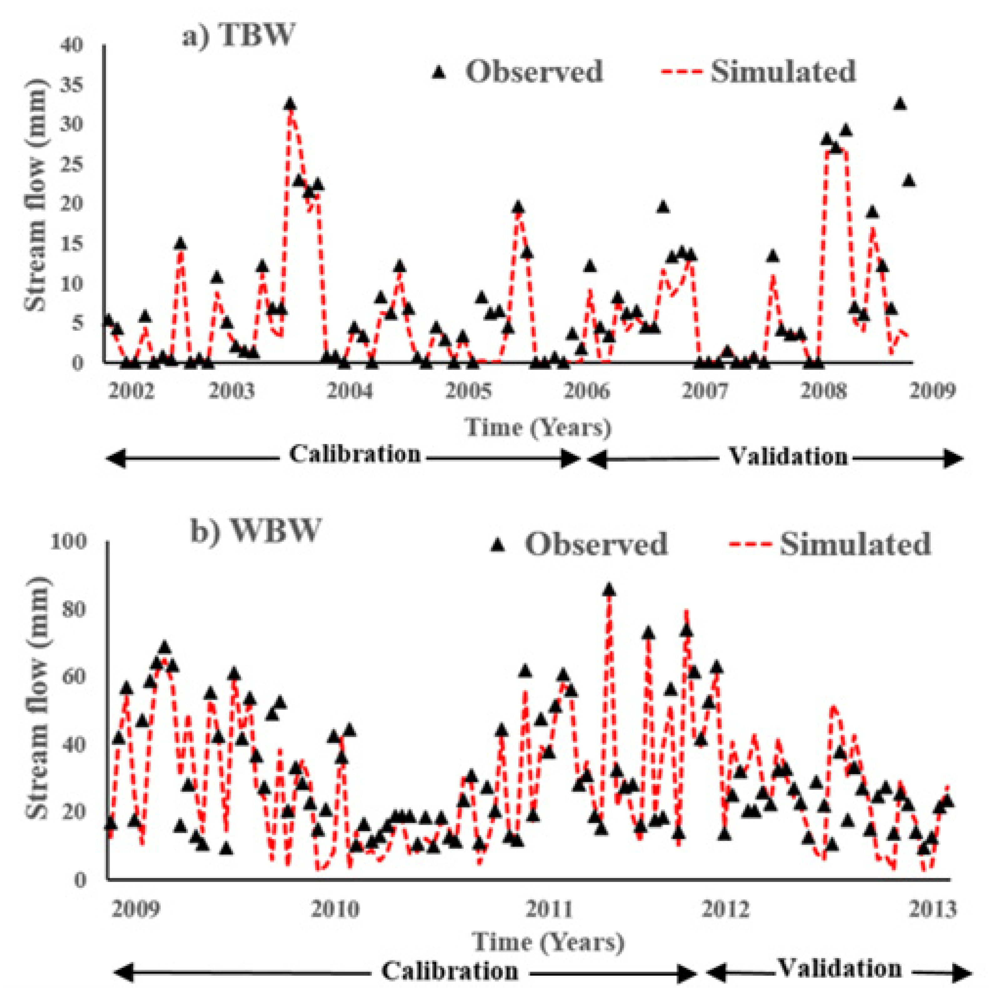
Figure 4.
The observed SY versus predictions of SY using CUSLE-KUSLE (Case 1), C-factor-KUSLE (Case 2), and C-factor-K-factor (Case 3) for the years between 2002 and 2013 for (a) TBW (n = 89) and (b) WBW (n = 139).
Figure 4.
The observed SY versus predictions of SY using CUSLE-KUSLE (Case 1), C-factor-KUSLE (Case 2), and C-factor-K-factor (Case 3) for the years between 2002 and 2013 for (a) TBW (n = 89) and (b) WBW (n = 139).
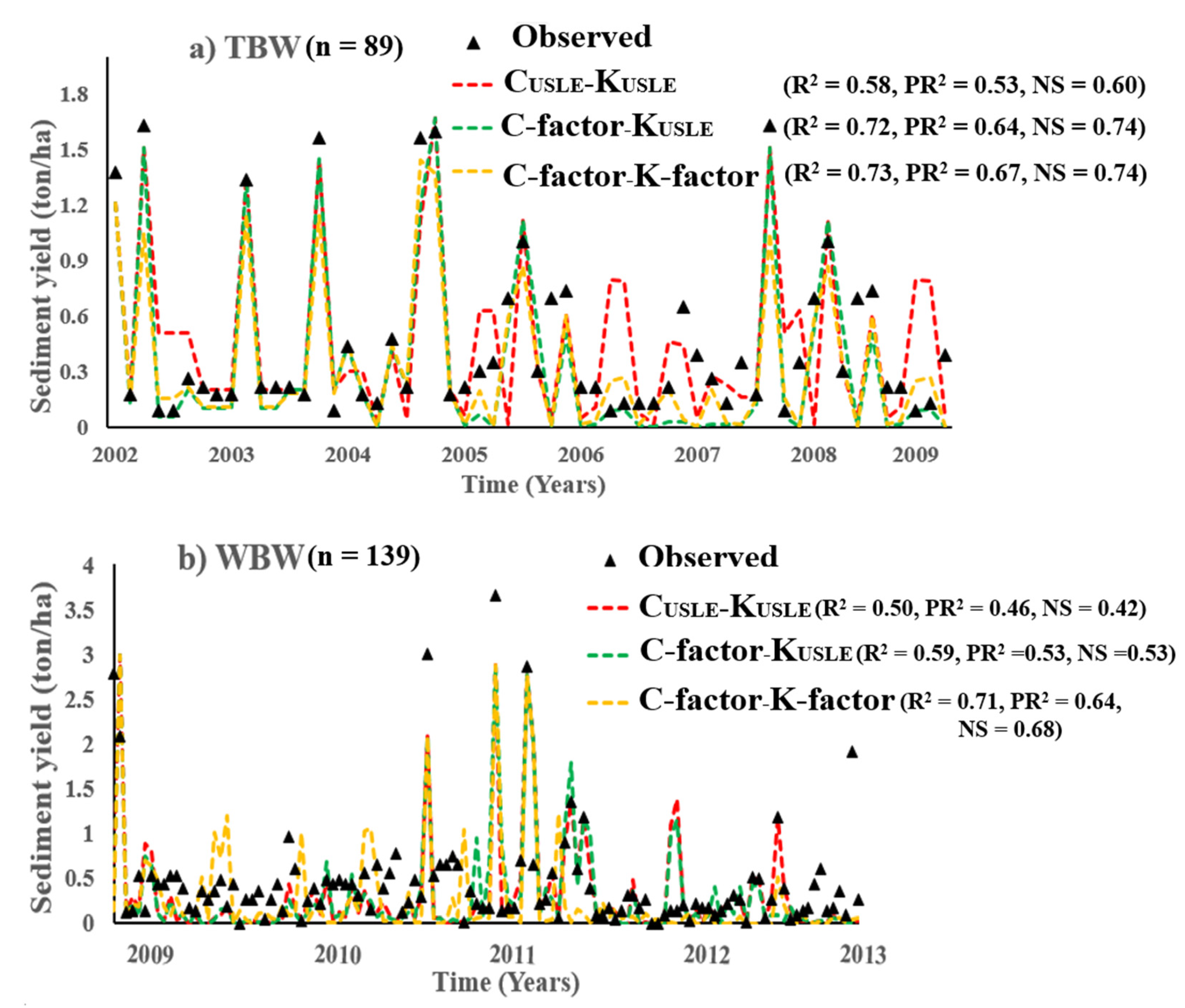
Figure 5.
HRU wise spatial distributions of the traditional CUSLE and KUSLE versus the average dynamic C and K factors in TBW from 2002 to 2009 (a,c) and WBW from 2009 to 2013 (b,d).
Figure 5.
HRU wise spatial distributions of the traditional CUSLE and KUSLE versus the average dynamic C and K factors in TBW from 2002 to 2009 (a,c) and WBW from 2009 to 2013 (b,d).

Figure 6.
Plots of time-series of annual averages of C-factor and K-factor for TBW (a,b) and WBW (c,d). (Solid and dashed lines indicate data points and trend lines, respectively).
Figure 6.
Plots of time-series of annual averages of C-factor and K-factor for TBW (a,b) and WBW (c,d). (Solid and dashed lines indicate data points and trend lines, respectively).
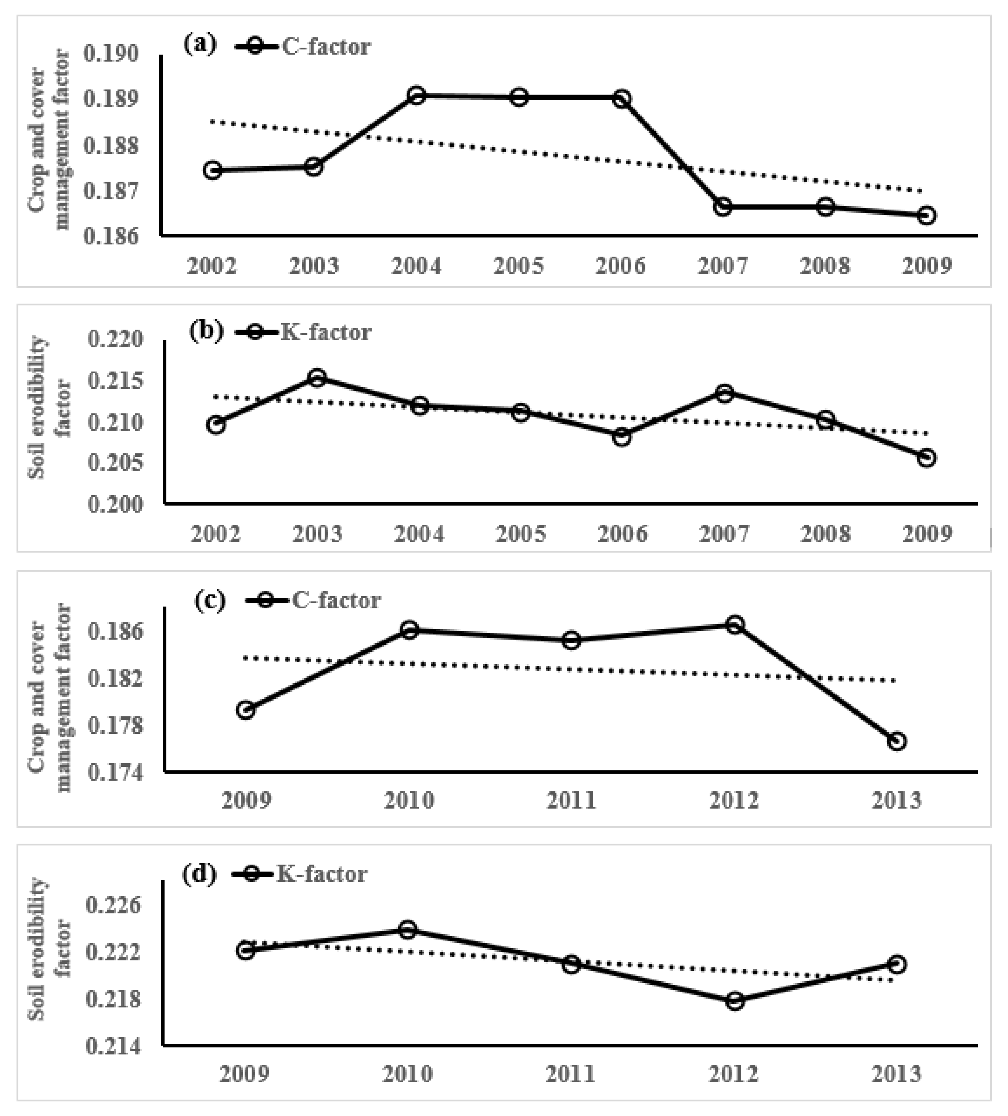
Figure 7.
Spatiotemporal distributions of the annual SY (ton/ha) in each HRU of TBW from 2002 to 2009 incorporating the dynamic models of C-factor and K-factor.
Figure 7.
Spatiotemporal distributions of the annual SY (ton/ha) in each HRU of TBW from 2002 to 2009 incorporating the dynamic models of C-factor and K-factor.

Figure 8.
Spatiotemporal distributions of the annual SY (ton/ha) in each HRU of WBW from 2009 to 2013 incorporating the dynamic models of C-factor and K-factor.
Figure 8.
Spatiotemporal distributions of the annual SY (ton/ha) in each HRU of WBW from 2009 to 2013 incorporating the dynamic models of C-factor and K-factor.

Table 1.
Input data used in SWAT modeling and estimation of the C-factor and K-factor.
| Data | Data Sources | Information | Period |
|---|---|---|---|
| DEM (S, LS) | NED | Raster, Annual, 30 m | 2002–2013 |
| Land cover | USGS: MODIS: LP DAAC | Raster, Annual, 500 m | 2002–2013 |
| Soil (BD, Psoil) | USDA | Raster, Annual, 60 m | 2002–2013 |
| EVI AWC LAI SR Meteorological data Hydrological data | USGS: MODIS: LP DAAC USGS: MODIS: LP DAAC USGS: MODIS: LP DAAC USGS: MODIS: LP DAAC U.S. National Weather Service, NOAA USGS | Raster, 16-Day, 250 m Raster, Monthly, 250 m Raster, 8-Day, 500 m Raster, 8-Day, 500 m Daily, 250 m Daily, 250 m Monthly | 2002–2013 2002–2013 2002–2013 2002–2013 2002–2013 2002–2013 |
Table 2.
Descriptive statistics of remotely sensed and modeled soil properties for K-factor estimation in TBW.
Table 2.
Descriptive statistics of remotely sensed and modeled soil properties for K-factor estimation in TBW.
| Descriptive Statistics | AWC (%) | BD (g/cm3) | Psoil (mm/h) | LS (m) | A (sq·km) |
|---|---|---|---|---|---|
| Mean | 13.82 | 1.20 | 497.02 | 23.88 | 258.32 |
| Median | 12.27 | 1.25 | 537.50 | 19.75 | 36.34 |
| Mode | 24.60 | 0.87 | 487.50 | 0.00 | 0.18 |
| Minimum | 0.00 | 0.29 | 0.12 | 0.00 | 0.09 |
| Maximum | 37.49 | 1.78 | 875.00 | 403.48 | 13,356.90 |
Table 3.
Descriptive statistics of remotely sensed and modeled soil properties for K-factor estimation in WBW.
Table 3.
Descriptive statistics of remotely sensed and modeled soil properties for K-factor estimation in WBW.
| Descriptive Statistics | AWC (%) | BD (g/cm3) | Psoil (mm/h) | LS (m) | A (sq·km) |
|---|---|---|---|---|---|
| Mean | 23.33 | 1.17 | 121.90 | 22.94 | 276.95 |
| Median | 22.84 | 1.14 | 116.75 | 7.03 | 35.73 |
| Mode | 18.25 | 1.44 | 39.25 | 0.30 | 0.09 |
| Minimum | 17.47 | 0.20 | 2.80 | 0.00 | 0.01 |
| Maximum | 32.80 | 1.55 | 887.50 | 1131.53 | 10,426.52 |
Table 4.
List of SWAT model calibration and validation parameters and the optimized values.
| Parameters | Descriptions | TBW | WBW | ||
|---|---|---|---|---|---|
| Ranges | Fitted Values | Ranges | Fitted Values | ||
| Stream flow | |||||
| ESCO | Soil evaporation compensation factor | 0.85–1.00 | 0.824 | 0.80–1.00 | 0.83 |
| CN2 | SCS curve number | 1.00–2.00 | 1.73 | 1.00–2.00 | 1.55 |
| AWCS | Available water capacity of the soil layer | 0.00–1.00 | 0.324 | 0.00–1.00 | 0.44 |
| Sediment yield | |||||
| ERORGN | Organic N enrichment ratio for loading with sediment | 0.00–5.00 | 0 | 0.00–4.00 | 0.5 |
| ERORGP | Phosphorus enrichment ratio for loading with sediment | 0.00–5.00 | 0 | 0.00–4.00 | 0.2 |
| HRU_SLP | Average slope steepness | 0.00–1.00 | 0.215 | 0.00–1.00 | 0.43 |
Table 5.
Summary of SWAT model calibration and validation results.
| Observed Data | Test | Simulation Period | Monitoring Station | Performance | |
|---|---|---|---|---|---|
| R2 | NS | ||||
| Stream Flow | Calibration | 2002–2005 | Rocky Creek | 0.842 | 0.711 |
| Validation | 2006–2009 | 0.786 | 0.680 | ||
| Calibration | 2009–2011 | Black River | 0.767 | 0.632 | |
| Validation | 2012–2013 | 0.598 | 0.620 | ||
| Calibration | 2009–2011 | Lynches River | 0.566 | 0.543 | |
| Validation | 2012–2013 | 0.587 | 0.518 | ||
| Calibration | 2009–2011 | Pee Dee River | 0.762 | 0.688 | |
| Validation | 2012–2013 | 0.655 | 0.645 | ||
| Sediment Yield | Calibration | 2002–2005 | Rocky Creek | 0.560 | 0.533 |
| Validation | 2006–2009 | 0.601 | 0.589 | ||
| Calibration | 2009–2011 | Black River | 0.662 | 0.644 | |
| Validation | 2012–2013 | 0.572 | 0.512 | ||
| Calibration | 2009–2011 | Lynches River | 0.442 | 0.360 | |
| Validation | 2012–2013 | 0.468 | 0.376 | ||
| Calibration | 2009–2011 | Pee Dee River | 0.691 | 0.564 | |
| Validation | 2012–2013 | 0.644 | 0.590 | ||
Table 6.
The performance results of the statistical evaluation for the implemented model cases.
| Performance Indices | TBW | WBW | ||||
|---|---|---|---|---|---|---|
| Case 1 | Case 2 | Case 3 | Case 1 | Case 2 | Case 3 | |
| NS | 0.603 | 0.741 | 0.744 | 0.418 | 0.527 | 0.683 |
| R2 | 0.582 | 0.719 | 0.733 | 0.503 | 0.594 | 0.713 |
| PR2 | 0.531 | 0.636 | 0.668 | 0.462 | 0.533 | 0.644 |
Publisher’s Note: MDPI stays neutral with regard to jurisdictional claims in published maps and institutional affiliations. |
© 2022 by the authors. Licensee MDPI, Basel, Switzerland. This article is an open access article distributed under the terms and conditions of the Creative Commons Attribution (CC BY) license (https://creativecommons.org/licenses/by/4.0/).
Share and Cite
MDPI and ACS Style
Preetha, P.; Al-Hamdan, A. A Union of Dynamic Hydrological Modeling and Satellite Remotely-Sensed Data for Spatiotemporal Assessment of Sediment Yields. Remote Sens. 2022, 14, 400. https://doi.org/10.3390/rs14020400
AMA Style
Preetha P, Al-Hamdan A. A Union of Dynamic Hydrological Modeling and Satellite Remotely-Sensed Data for Spatiotemporal Assessment of Sediment Yields. Remote Sensing. 2022; 14(2):400. https://doi.org/10.3390/rs14020400
Chicago/Turabian StylePreetha, Pooja, and Ashraf Al-Hamdan. 2022. "A Union of Dynamic Hydrological Modeling and Satellite Remotely-Sensed Data for Spatiotemporal Assessment of Sediment Yields" Remote Sensing 14, no. 2: 400. https://doi.org/10.3390/rs14020400
Note that from the first issue of 2016, this journal uses article numbers instead of page numbers. See further details here.