Application of the Crow Search Algorithm to the Problem of the Parametric Estimation in Transformers Considering Voltage and Current Measures

Abstract

The problem of the electrical characterization of single-phase transformers is addressed in this research through the application of the crow search algorithm (CSA). A nonlinear programming model to determine the series and parallel impedances of the transformer is formulated using the mean square error (MSE) between the voltages and currents measured and calculated as the objective function. The CSA is selected as a solution technique since it is efficient in dealing with complex nonlinear programming models using penalty factors to explore and exploit the solution space with minimum computational effort. Numerical results in three single-phase transformers with nominal sizes of 20 kVA, 45 kVA, 112.5 kVA, and 167 kVA demonstrate the efficiency of the proposed approach to define the transformer parameters when compared with the large-scale nonlinear solver fmincon in the MATLAB programming environment. Regarding the final objective function value, the CSA reaches objective functions lower than $2.75\times {10}^{-11}$ for all the simulation cases, which confirms their effectiveness in minimizing the MSE between real (measured) and expected (calculated) voltage and current variables in the transformer.

1. Introduction

1.1. General Context

Nowadays, electricity service plays one of the most important roles in the technological developments of the 4.0 industrial revolution since electrical distribution grids in both urban and rural areas grow as per the requirements of the industry and society [1,2]. Owing to the accelerated growth of distribution networks, these networks present a high level of new devices involved in their development, such as protective devices, transformers, distribution lines, shunt compensators, and dispersed sources [3], among others. Nevertheless, the expansion of these grids has significant impacts on the energy quality mainly observed in the high increments in the total grid power losses that are mostly caused in distribution lines and transformers with low chargeability [4,5]. In developed countries, expected energy losses in transformers are about $3\%$ [6]; however, in Latin American countries, the level of power losses in distribution networks can be between 6% and 18%, with most of them being caused in the distribution transformers due to their low loadability levels, which is an important problem that utilities have started to focus in the past few years [4,7].

In the Colombian context, between 2010 and 2018, the number of transformers installed in medium-voltage levels increased by about $31\%$, i.e., 58,1592 new transformers were added in 8 years [4]. This significant increment in the number of transformers demonstrates that studies regarding the efficiency of electrical distribution networks are required to define the real contribution of these devices in total energy losses wasted in the distribution activity, since in the Colombian systems, more than the 50% of the total distribution energy losses are assigned to the transformers [8].

1.2. Motivation

Currently, the transformer within an electrical energy system is of vital importance due to the benefits it provides, such as change in voltage levels and its high efficiency [9]. It is for this reason that improper functioning or failure in its operations affects the reliability and efficiency of the entire system is associated with these devices [5]. Consequently, we are interested in studying transformers by means of models that represent their performance under different conditions where the efficiency and losses of the transformer are analyzed. In this process of determining electrical losses, it is mandatory to know its electrical parameters since with them it is possible to determine the electrical performance of the transformer [9]. The use of electrical transformers in distribution networks is quite common due to the characteristics offered by its operation; however, similar to all equipment that is exposed to different situations in its operating life, a transformer generates wear and tear, which consequently changes its initial parameters. This shortens its lifespan as well as deteriorates its initial efficiency [10]; this must not exceed the limits established by the norms in Colombia, such as in the NTC 3445 for the case of transformers [11] and in the CREG (Energy and Gas Regulation Commission) [8].

In order to determine the transformer parameters, the traditional method based on short-circuit and open-circuit tests is used in transformers, which requires disconnecting the system, making it impractical since they are used by multiple users in the distribution grids [12]. Observing this panorama, this research work arises from an interest in monitoring these parameters through voltage and current measurements that are already taken in said system to have traceability, coordination, and operation of the protection devices. From this, the necessary data to determine the losses in the transformers under different operating conditions can be obtained using noninvasive tests [13]. To solve the problem of the parametric estimation in single-phase transformers, we propose the application of a continuous metaheuristic optimizer based on the crows’ behavior known as the crow search algorithm (CSA). The main contribution of this research is focused on the usage of voltage and current measurements taken at the transformers’ terminals, which help avoid service interruption as these measurements are taken directly from the transformer operation site [8].

1.3. Review of the State-of-the-Art

In the current literature, it has proposed multiple approaches to determine all the electrical parameters in transformers that are based on nonintrusive approaches mainly focused on voltage and current measurements at their terminals.

Authors of [14] proposed a real-time approach to determine the electrical parameters using two-terminal synchronized voltage and current measurements obtained through a transformer intelligent electronic device. With these measurements, it is possible to estimate the transformer’s fundamental parameters, including turns ratio, series winding resistance, series leakage inductance, shunt magnetizing inductance, and shunt core loss resistance, among others, considering less than one cycle current and voltage data. The authors modified the conventional mean square error method by introducing a recursive approach. Numerical implementations showed that the proposed approach reached less than 10% errors with respect to the real transformer data presented in [15]. Authors of [16] proposed an implementation of a measured interfaced in terminals of the transformer based on the LabVIEW-FPGA technology. This interface uses the Fourier transform to obtain the voltage and current input/outputs of the transformer. These data were fed to a mathematical model that calculated the mean square error between the expected values and the measured ones. The effectiveness of the proposed approach was validated using classical transformer short-circuit and open-circuit tests. Bocanegra et al. in [8] proposed the solution to the parameters estimation problems in single-phase transformers using a real variable optimization model that minimizes the mean square error between the voltage and current measures and their expected values. The proposed optimization model was implemented in the General Algebraic Modeling System (i.e., GAMS). Numerical results in three test transformers from 20 kVA to 112.5 kVA show the effectiveness of the proposed optimization model with objective function values less than $1\times {10}^{-10}$ for all the test cases.

Authors of [17] have presented the application of the black-hole optimization algorithm to solve the problem of the parametric estimation in single-phase transformer using voltage and current measures. Numerical results demonstrate the effectiveness and robustness of the black-hole optimizer regarding final objective function values when compared with classical methods such as particle swarm optimization and gravitational search algorithm, among others. In [4], the authors proposed the application of the sine–cosine algorithm for the parametric estimation in single-phase transformers using voltage and current measures. Numerical results were compared with the GAMS approach in [8], which demonstrated that combinatorial methods are excellent tools for replacing commercial solvers with excellent numerical performance where the objective function in all the test transformers was less than $1\times {10}^{-11}$. Other approaches in the field of metaheuristics applied to the studied problem are listed in

Table 1. Main literature approaches applied to the problem of parametric estimation in single-phase transformers.

Optimization Method	Reference	Year
Particle swarm optimization and genetic algorithms	[18]	2014
Mean square recursive method	[14]	2016
Mean square with estimation window	[16]	2016
Imperialist competitive and gravitational search algorithms	[10]	2017
Coyote optimization algorithm	[19]	2020
General algebraic modeling system	[8]	2020
Manta ray foraging optimization	[20]	2020
Slime mold optimizer	[21]	2021
Black-hole optimization	[17]	2021
Sine–cosine algorithm	[4]	2021

.

The main characteristic of the optimization methods reported in Table 1 is that all of them use optimization techniques to estimate the electrical parameters in single-phase transformers only considering voltage and current measures, which make these methodologies suitable for use in multiple applications without having to move transformers to a laboratory to apply the classical short-circuit and open-circuit tests. Note that most of the algorithms presented in Table 1 are from the metaheuristic family, which is an opportunity of research that this study has explored with the application of a new optimization method as is described in the next subsection.

1.4. Contributions and Scope

The main contributions of this research are: (i) the application of the crow search algorithm to the parametric estimation in single-phase transformers using voltage and current measures at terminals of the transformer under nominal operative conditions; (ii) the computational validation of the studied optimization model with the large-scale nonlinear solver fmincon from MATLAB and multiple metaheuristics recently reported in the current literature. The comparison between these solution strategies demonstrates the effectiveness and robustness of the CSA to deal with the studied problem with low-computational effort and high-quality performance since the objective function is less than $2.75\times {10}^{-11}$ for all the transformers studied.

In this research, the crow search algorithm is selected as the combinatorial optimization methodology to solve the studied problem based on the following facts: (i) The CSA is a metaheuristic optimization method from the family of bio-inspired algorithms that presents a balanced performance between the exploration and exploitation of the solution space, using memories to maintain and present the most promissory solutions of the solution space, as well as generating new solutions that allow to explore nonvisited solution regions; (ii) the effectiveness and robustness of the CSA to solve nonlinear nonconvex optimization problems has recently been demonstrated in similar optimization problems such as parametric estimation in photovoltaic modules [22], parametric estimation in induction motors [23], optimal phase-swapping in electrically unbalanced distribution networks [24], and segmentation of magnetic resonance images [25], among others; (iii) In the current literature, there is no evidence of the application of the CSA to the problem addressed in this research, which is an opportunity of research to which this paper tries to contribute.

It is worth mentioning that in this research, it is considered that all the voltage and current measures in terminals of the transformer were taken from specialized personnel of the distribution company in the place of transformer works [4]. These measures are passed through a filtering process to reduce the possibility of measurement errors and spurious data [17]. The filtering process is a key factor to ensure the efficiency of the proposed estimation methodology; however, note that the CSA is independent of the input information as this information is noncontrollable during the research process; the quality of the final solution, however, will be highly dependent on these inputs.

1.5. Document Organization

This document is structured as follows: Section 2 presents the mathematical derivation of the nonlinear programming model that represents the problem of parametric estimation. This model is entirely developed with the application of Kirchhoff’s laws to the equivalent electric circuit of the transformer [8]. Section 3 describes the main aspects of the solution methodology based on the application of CSA. Section 4 shows the main characteristics of the test transformers that have nominal capabilities of 20 kVA, 45 kVA, 112.5 kVA, and 167 kVA, and presents all the numerical analyses after the application of the CSA to the studied problem as well as its comparisons with the fmincon solver in the MATLAB programming environment and recently metaheuristics available in the current literature. Finally, Section 5 presents the main concluding remarks derived from this research work.

2. Mathematical Formulation

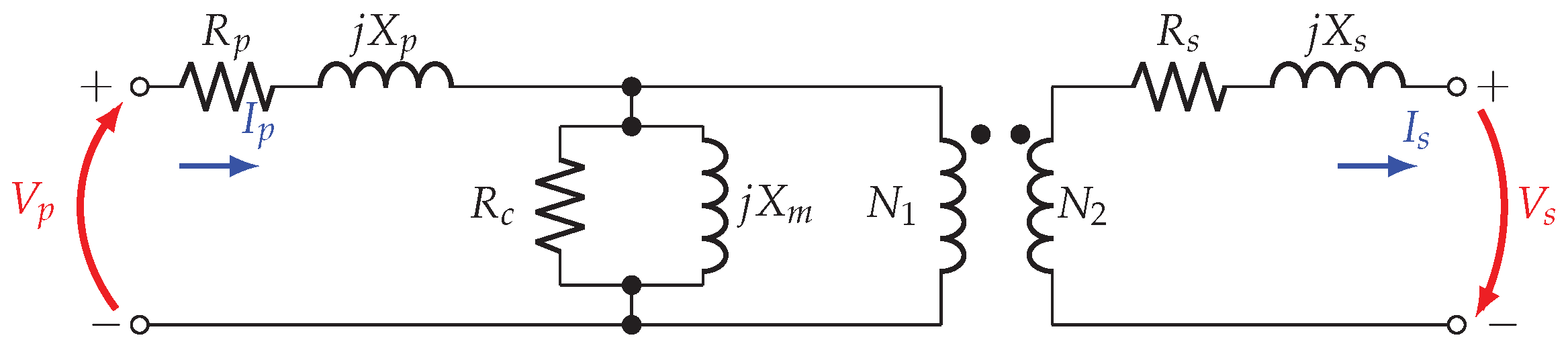
To develop the mathematical optimization model that represents the problem of the parametric estimation in single-phase transformers, we consider the electrical equivalent of the transformer presented in Figure 1 [12]. Note that the electrical representation of the transformer includes two series branches that are associated with the copper losses in the primary and secondary windings ($R_p$ and $R_s$ resistances) as well as their magnetic flow dispersions (i.e., $X_p$ and $X_s$ reactances). In the case of the magnetic core of the transformer, the resistance $R_c$ models the active power losses caused by the parasitic currents induced along the metal plates that conform the transformer core; while the reactance $X_m$ models the magnetic flow losses caused by the hysteresis process in the complete cycle of the sinusoidal input (i.e., magnetization current) [12].

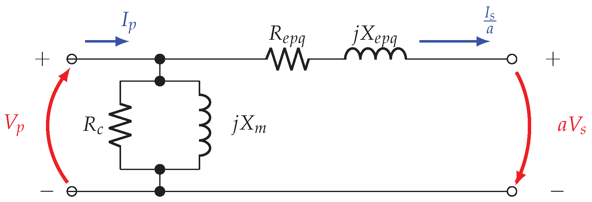
With the aim of simplifying the equivalent of the transformer, all the components from the secondary site are referred to the primary side (see Equations (1)–(3)); in addition, based on the recommendation in [8] for typical applications of the transformers in distribution levels, the magnetization branch can be directly connected to the transformer input, which allows the two series branches to become equivalent to one branch [4]. The simplified transformer model is depicted in Figure 2. It is worth mentioning that the movement in the magnetization branch is possible, since the total current through this branch under nominal operative conditions is as much as 3% of the input current [12].

$$\begin{array}{c}\hfill a=\frac{V_p}{V_s},\end{array}$$

(1)

$$\begin{array}{c}\hfill R_{epq}=R_p+a^2{R}_s,\end{array}$$

(2)

$$\begin{array}{c}\hfill X_{epq}=X_p+a^2{X}_s,\end{array}$$

(3)

where a is the ideal transformer relationship between primary and secondary sides, and $R_{epq}$ and $X_{epq}$ correspond to the equivalent resistances and reactances of the equivalent series branch.

From the equivalent circuit of the transformer depicted in Figure 2, the set of constraints associated with Kirchhoff’s laws applied in its complex form is obtained as listed below.

$$\begin{array}{c}\hfill I_{sp}=\frac{I_s}{a}=\frac{V_p}{R_{eqp}+R_L+j\left(X_{eqp}+X_L\right)},\end{array}$$

(4)

$$\begin{array}{c}\hfill I_p=I_{sp}+\frac{X_m-j{R}_c}{R_c{X}_m}{V}_p,\end{array}$$

(5)

$$\begin{array}{c}\hfill V_{sp}=a{V}_s=(R_L+j{X}_L)I_{sp},\end{array}$$

(6)

where $I_{sp}$ represents the current in the secondary side of the transformer as seen in the primary side, $V_{sp}$ is the voltage in the secondary terminals of the transformer as referred to the primary side; $R_L$ and $X_L$ are the equivalent impedance loads referred to the primary side. Note that Equation (4) represents the current calculation in the secondary side of the transformer as a function of the voltage input $V_p$. This equation is obtained by using a current division connected to the load impedance in $V_{sp}$ terminals. Equation (5) defines the total current input, which is obtained by applying the first Kirchhoff’s law at the node connected to the series and parallel impedances of the transformer. Equation (6) is defined with the application of Kirchhoff’s second law at terminals of the load.

Owing to the objective in the studied problem corresponds to the determination of the electrical parameters of the transformer, i.e., $R_C$, $X_m$, $R_{eqp}$, and $X_{eqp}$, these variables are defined among their minimum and maximum bounds [17]. These box-type constraints are listed from (7) to (10).

$$\begin{array}{c}\hfill R_C^{min}\le R_C\le R_C^{max},\end{array}$$

(7)

$$\begin{array}{c}\hfill X_m^{min}\le X_m\le X_m^{max},\end{array}$$

(8)

$$\begin{array}{c}\hfill R_{eqp}^{min}\le R_{eqp}\le R_{eqp}^{max},\end{array}$$

(9)

$$\begin{array}{c}\hfill X_{eqp}^{min}\le X_{eqp}\le X_{eqp}^{max},\end{array}$$

(10)

where $y^{min}$ and $y^{max}$ represent the lower and upper bounds of the decision variable y. An additional constraint reported in [8,17] is related with the predominant effect of the inductive series’ parameters regarding the series inductance. This constraint is defined as presented in (11).

$$\begin{array}{c}\hfill X_{eqp}-\beta R_{eqp}\ge 0,\end{array}$$

(11)

where $\beta$ is bigger than 1.

Now the aim of the proposed study is to determine the electrical parameters of a single-phase transformer that minimizes the mean square error between the measured and calculated voltages and currents in the transformer terminals. To do so, we employ the objective function proposed in [8], which is defined in (11).

$$min{z}_{\mathrm{MSE}}=\frac{1}{2{\left(I_p^m\right)}^2}{\left(\left|I_p\right|-I_p^m\right)}^2+\frac{1}{2{\left(I_{sp}^m\right)}^2}{\left(\left|I_{sp}\right|-I_{sp}^m\right)}^2+\frac{1}{2{\left(V_{sp}^m\right)}^2}{\left(\left|V_{sp}\right|-V_{sp}^m\right)}^2$$

(12)

where $I_p^m$, $I_{sp}^m$, and $V_{sp}^m$ are the current measures in the primary and secondary sides of the transformer as well as the voltage output in its secondary side, respectively. Note that we assume that the input voltage corresponds to the nominal transformer voltage, and the error between its measured and theoretical value is zero.

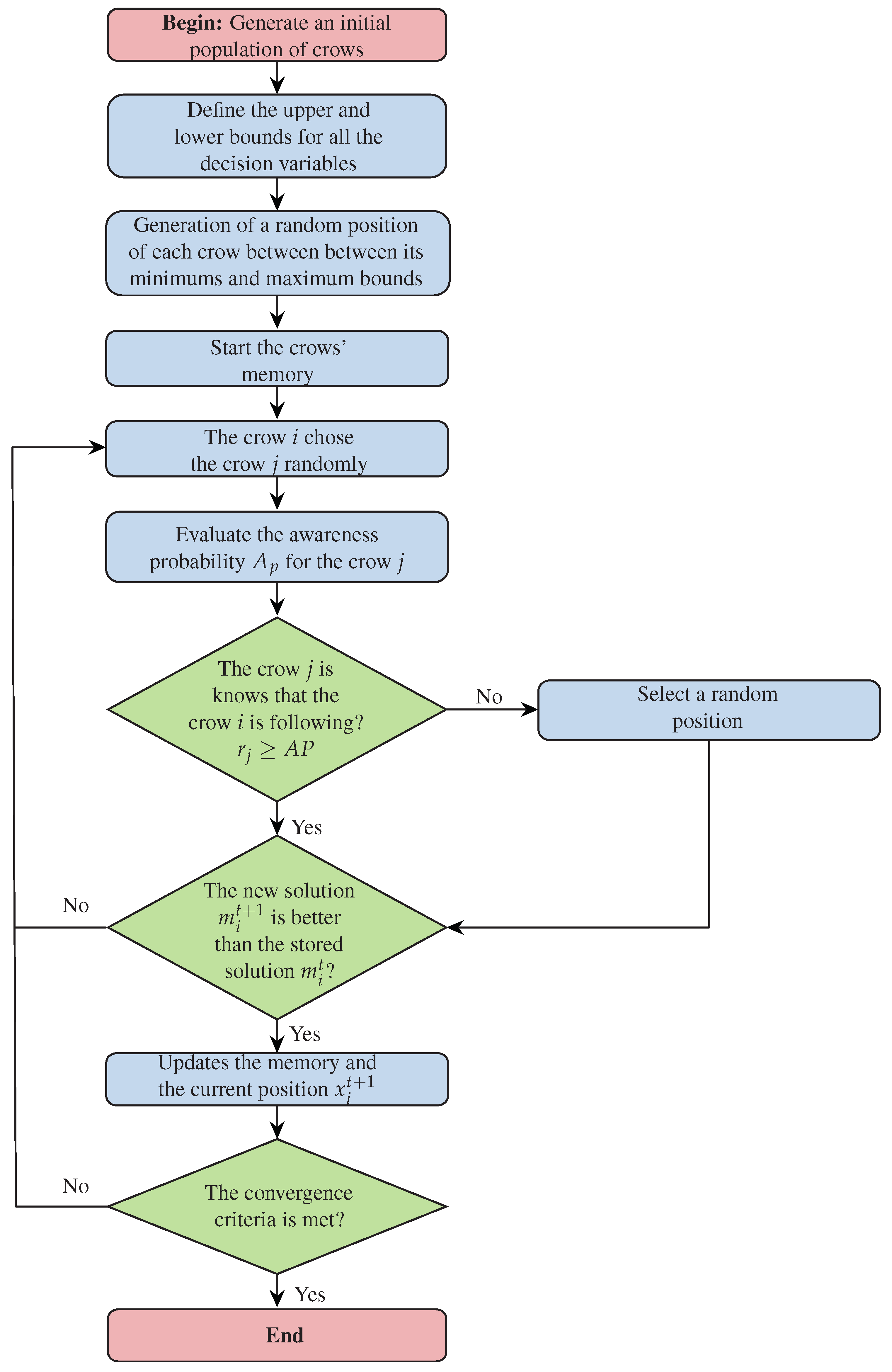
Remark 1.

The optimization problem defined with the objective function (12) subject to the set of constraints (4) to (11) is a nonlinear programming model that can provide multiple local optimal solutions due to the nonconvexity of the solution space [17].

These complexities in the optimization model make necessary the usage of advanced optimization techniques to find the best optimal solution possible with minimum computational effort; for this reason, in this research is proposed the application of the CSA to solve the problem of the exact nonlinear programming model. All the details of the CSA are discussed in the next section.

3. Solution Methodology Proposed

To deal with the problem of parametric estimation in single-phase transformers modeled in the previous section, this research proposes the application of the recently developed metaheuristic optimization algorithm known as the crow search algorithm [22,26]. The main idea of the CSA is to model the way crows search (steal) for their food and store it in secret places [27,28]. The main characteristics of the CSA are described below.

3.1. Crow Search Algorithm

The CSA is a bio-inspired metaheuristic optimization algorithm that is based on the behaviors of crows in their living communities. Crows are considered the smartest animals among birds. They have the ability to remember faces, identify potential dangers in near areas, as well as the capacity to steal food and store it in secret places [26]. To steal food, a crow spends long periods of time observing other crows to find the places where they store their food. In addition, these birds have incredible memory capacity as they can remember the places where the food was stored weeks or months later. The main characteristics of crows are listed below:

• Crows live in herds.
• They keep their food in secret places and search for food kept by other crows.
• They trick other crows with random movements to keep their food safe.

Figure 3 presents the process carried out by the ith crow to follow the movements of the jth crow. Note that the length of the flight is determined by the $f_l$ factor, where values less than 1 represent short movements (local exploration), and values grater than 1 represent big movements through the solution space (global exploration).

As observed in Figure 3, the ith crow follows the jth crow to know the location of the food kept by jth crow in order to steal it and transport it to a new safe place. The position of the crow i, i.e., $x(i,t)$, can have two possible states as a function of the possibility that the crow j knows that it is being followed. This situation is governed by the awareness probability factor, i.e., $A_p$ [22].

The following steps are essential to implement the CSA to solve combinatorial optimization problems [26].

3.1.1. Initial Population and Memory Generation

As a classical population-based metaheuristic optimizer, the CSA explores and exploits the solution space by making the initial population evolves. This initial population is randomly generated with the structure presented below:

$$X_t=\left[\begin{array}{cccc}{x}_1^1& x_2^1& \cdots & x_d^1\\ x_1^2& x_2^2& \cdots & x_d^2\\ ⋮& ⋮& ⋮& ⋮\\ x_1^N& x_2^N& \cdots & x_d^N\end{array}\right]$$

(13)

The CSA is characterized by the usage of memories, where each crow $x_{i,t+1}$ has information regarding the position of the largest food pantry during the exploration and exploitation of the solution space. The memories of the crows take the following form:

$$M_t=\left[\begin{array}{cccc}{m}_1^1& m_2^1& \cdots & m_d^1\\ m_1^2& m_2^2& \cdots & m_d^2\\ ⋮& ⋮& ⋮& ⋮\\ m_1^N& m_2^N& \cdots & m_d^N\end{array}\right]$$

(14)

Note that initially, the memories are assigned with the values of the initial population, since in the first iteration, every crow is starting its exploration of the solution space.

3.1.2. Evaluation of the Fitness Function

The CSA, similar to any combinatorial optimization technique, explores and exploits the solution space by using a modification of the objective function named as the fitness function [22]. This function allows including all the constraints using penalty factors. The proposed fitness function in this research is presented below.

$$\begin{array}{c}\hfill F_f=z_{\mathrm{MSE}}-{\theta }_{1}min\left\{X_{eqp}-\beta R_{eqp},0\right\}\end{array}$$

(15)

where ${\theta }_1$ is a penalty factor associated with the violation of the predominant inductive characteristic of the transformer, which is the only inequality constraint that requires to be included in the fitness function [4].

Note that the remaining constraints, i.e., (7)–(10), are maintained as feasible during the exploration and exploitation of the solution space using rules that limit all the decision variables to their respective lower and upper bounds. In the case of equality constraints (4) to (6), these are always feasible as no restrictions regarding the voltage and current variables are required in the studied optimization problem.

3.1.3. Movements of the Crows through the Solution Space

The movement of the crow i, i.e., $x_{i,t+1}$, as mentioned earlier, is governed by the awareness probability ($A_p$). In this sense, the crow i uses a random coefficient $r_j$ that defines the probability of following the jth crow to discover the position of its food $m_{j,t}$. The evolution rule takes the following form:

$$X_{i,t+1}=\left\{\begin{array}{c}\mathrm{if}{r}_j\ge A_p,\mathrm{then}:x_{i,t}+r_i\times f{l}_{i,t}\times (m_{j,t}-X_{i,t})\\ \mathrm{otherwise},\mathrm{a}\mathrm{random}\mathrm{exploration}\mathrm{is}\mathrm{made}\end{array}\right.$$

(16)

where $r_i$ and $r_j$ are random numbers with normal distribution contained between 0 and 1.

3.1.4. Memory Updating

To preserve the information regarding the best food pantries, each crow has the possibility of updating the memory $m_{i,t}$ as a function of the objective function obtained for $x_{i,t+1}$ as described below.

$$m_{i,t+1}=\left\{\begin{array}{c}{x}_{i,t+1},\mathrm{if}f\left(x_{i,t+1}\right)\ge f\left(m_{i,t}\right)\\ \mathrm{Otherwise}{m}_{i,t}\end{array}\right.$$

(17)

where $f\left(x_{i,t+1}\right)$ is the objective function value of the offspring individual $x_{i,t+1}$.

3.2. Ending of the Search Process

The exploration and exploitation of the solution space end when one of the following criteria is met.

• The best memory in $M_t$, i.e., the position that generates the minimum value of the objective function does not improve after $k_{max}$ consecutive iterations.
• When the total number of iterations $t_{max}$ has been reached.

Note that $k_{max}$ is assigned as 20% of the number of iterations.

3.3. Application of CSA to the Studied Problem

The general flow diagram that represents the application of CSA to the problem of parametric estimation in single-phase transformers considering voltage and current measures is presented in Figure 4.

An important stage regarding the setting of the proposed CSA to solve the studied problem corresponds to the parameter adjustment of the algorithm, i.e., the number of iterations ($t_{max}$), the awareness factor ($A_p$), the population size ($N_i$), and the number of evaluations ($N_e$). To determine the best set of parameters, 50 consecutive evaluations of the CSA were made, in which the final objective function value and the processing times required when the population sizes, the awareness factor and the number of iterations are varied. The numerical performance in these tests are depicted in Figure 5. Note that the set of parameters selected (see zoomed area in Figure 5) present an adequate performance between the final objective function value and the total processing times. The selected parameters are: $A_f=0.80$, $t_{max}=50$, $N_e=50$, and $N_i=25$. The main advantage with these parameters is that the expected execution time is about 1 s.

4. Test Transformers and Numerical Validations

The computational validation of the proposed methodology is achieved through the implementation of the CSA in three different transformers reported in [8]. These transformers have sizes of 20 kVA, 45 kVA, 112.5 kVA, and 167 kVA, respectively. The computational validations have been stored in a personal computer AMD-A10 9520P RADEON R5, 10 COMPUTE CORES 4C+6G 2.50GHz, 16 GB RAM, 64 bits, with Windows 10 Home Single Language using the MATLAB programming environment version $2121a$.

4.1. First Test Transformer 20 kVA

This transformer has a nominal power rate of 20 kVA, with 8000 V/240 V of input/output voltage magnitudes, operated at 60 Hz, and is assigned the $\beta$-factor greater or equal to 3 [8]. The measured current and voltages for this transformer as well as its nominal load values are reported in

Table 2. Measured voltage and currents for the first test transformer.

Parameter	Value	Unit
$I_p^m$	2.5369	A
$I_{sp}^m$	2.466	A
$V_{sp}^m$	7891.2811	V
$V_p$	8000	V
$R_L$	3200	$\Omega$
$X_L$	0	$\Omega$

. In addition,

Table 3. Lower and upper bounds admissible for the decision variables.

Parameter	${\mathit{x}}^{min}$ ($\mathbf{\Omega }$)	${\mathit{x}}^{max}$ ($\mathbf{\Omega }$)
$R_c$	140,000	180,000
$X_m$	30,000	50,000
$R_{eqp}$	30	50
$X_{eqp}$	150	250

presents the upper and lower bounds for the decision variables.

Numerical results show that for the first test transformer, a final objective function value of $2.640532\times {10}^{-11}$ is reached with an average processing time about 976.32 ms. Furthermore, the solution with respect to the transformer parameters is completely feasible since all the parameters are within their bounds (see Table 3). In addition, observe that constraint (11) is completely fulfilled:

$$\begin{array}{c}\hfill X_{eqp}-\beta R_{eqp}=198.5632-3\times 38.0209=84.501\ge 0\end{array}$$

(18)

Regarding the objective value, we can confirm that for this test transformer, the optimal solution found by the CSA can be considered near-optimal, since it is very close to zero. After comparing the calculated and real values (taken from [12]) in Figure 6, the maximum error with respect to the core resistance stands at about $4.87\%$. However, the value provided by the CSA presents high quality, since we find that once all the parameters obtained by our proposal are evaluated in the optimization model, the variables $I_p$, $I_{sp}$, and $V_{sp}$ have a maximum estimation error about $5.10\times {10}^{-4}$, which is the error for the secondary voltage profile on the primary side, i.e., $V_{sp}$; conversely, the estimation error for the currents is zero with four decimals in the analysis.

It is worth mentioning that it is the nonconvexity of the solution space of the optimization model studied in this research that makes it possible to find multiple solutions with minimum objective function values that can be considered as in the case of the CSA near-optimal values. To show this fact,

Table 4. Comparison between the CSA approach and the fmincon solver from MATLAB.

Parameter/Variable	Relative Error CSA vs. Real Data (%)	Relative Error Fmincon vs. Real Data (%)
$R_c$	3.968969497	0.621291572
$R_m$	4.869202865	4.128448698
$R_{eqp}$	0.987239583	4.092187500
$X_{eqp}$	3.418333333	13.09098958
$I_p$	0	0
$I_{sp}$	0	0
$Vsp$	0.000514492	0.001027717

provides the relative errors between the real data and our approach as well as the results obtained with the fmincon solver from MATLAB.

Relative errors listed in Table 4 clearly show that the proposed CSA maintains relative errors of less than $5\%$, whereas the fmincon solver has a maximum relative error of about $13\%$ in the case of the magnetization reactance. In addition, the estimation error of the transformer variables shows that the fmincon has an error of $1.028\times {10}^{-3}$, whereas in the proposed approach, an error of about $5.14\times {10}^{-4}$ in the case of the secondary voltage variable was found, which confirms the CSA’s effectiveness to estimate the parameters in the first test transformer.

4.2. Second Test Transformer 45 kVA

This transformer has a nominal apparent power rate of about 45 kVA, with 11,400 V/240 V of input/output voltage magnitudes, which is operated at 60 Hz. For this transformer, the $\beta$-factor is assigned greater or equal to 4 [8]. The measured currents and voltages for this transformer as well as its nominal load values are reported in

Table 5. Measured voltage and currents for the second test transformer [8].

Parameter	Value	Unit
$I_p^m$	3.9452	A
$I_{sp}^m$	3.8774	A
$V_{sp}^m$	11,198.0402	V
$V_p$	11,400	V
$R_L$	2888	Ω
$X_L$	0	Ω

. In addition,

Table 6. Lower and upper bounds admissible for the decision variables [8].

Parameter	${\mathit{x}}^{\mathit{real}}$ ($\mathbf{\Omega }$)	${\mathit{x}}^{min}$ ($\mathbf{\Omega }$)	${\mathit{x}}^{max}$ ($\mathbf{\Omega }$)
$R_c$	220,000	100,000	300,000
$X_m$	64,500	30,000	80,000
$R_{eqp}$	45	30	70
$X_{eqp}$	204	100	300

presents the upper and lower bounds for the decision variables.

Once the CSA is applied to this test transformer, a final objective function value of $2.368717\times {10}^{-11}$ is obtained with an average processing time about 957.16 ms. Note that the solution regarding the transformer parameters is completely feasible since all the parameters are within their bounds (see Table 6). In addition, observe that constraint (11) is completely fulfilled:

$$X_{eqp}-\beta R_{eqp}=207.6435\Omega -4\times 44.7587\Omega =25.6087\Omega \ge 0$$

(19)

Additionally, when we compare the calculated and real values (taken from [12]) in Figure 7, the maximum error with respect to the core resistance is about $4.38\%$ (see

Table 7. Comparison between the CSA approach and the fmincon solver from MATLAB for the second transformer test.

Parameter/Variable	Relative Error CSA vs. Real Data (%)	Relative Error Fmincon vs. Real Data (%)
$R_c$	2.191509591	4.801995818
$X_m$	4.387300155	10.58551628
$R_{eqp}$	0.536222222	0.076
$X_{eqp}$	1.786029412	0.134705882
$I_p$	0	0
$I_{sp}$	0	0
$V_{sp}$	0.000486692	0.000973385

). However, the value provided by the CSA presents high quality, since we find that once all the parameters obtained by our proposal are evaluated in the optimization model, the variables $I_p$, $I_{sp}$, and $V_{sp}$ have a maximum estimation error about $4.87\times {10}^{-4}$, which is the error for the secondary voltage profile on the primary side, i.e., $V_{sp}$; conversely, the estimation error for the currents is zero with four decimals in the analysis.

Note that Table 7 presents the relative error between the real data and our approach as well as the results obtained with the MATLAB solver fmincon.

The related errors listed in Table 7 clearly show that the proposed CSA keeps the relative error below $5\%$, while the solver fmincon has a maximum relative error of approximately $10.6\%$ in the case of equivalent resistors of the equivalent series branch. Furthermore, the estimation error of the transformer variables shows that fmincon has an error of $9.73\times {10}^{-4}$, while the proposed approach has an error of approximately $4.87\times {10}^{-4}$ in the case of secondary voltage variable; this confirms he CSA’s effectiveness in estimating the parameters in the second test transformer.

4.3. Third Test Transformer 112.5 kVA

This transformer has a nominal apparent power rate of 112.5 kVA, with 13200/440 V of input/output voltage magnitudes, operated at 60 Hz, with a $\beta$-factor greater or equal to 4 being assigned to it [8]. The measured current and voltages for this transformer as well as its nominal load values are listed in

Table 8. Measured voltage and currents for the third test transformer.

Parameter	Value	Unit
$I_p^m$	7.9032	A
$I_{sp}^m$	7.7484	A
$V_{sp}^m$	12,000.7485	V
$V_p$	13,200	V
$R_L$	1341.3001	$\Omega$
$X_L$	774.4	$\Omega$

. In addition,

Table 9. Lower and upper bounds admissible for the decision variables for the third test.

Parameter	${\mathit{x}}^{\mathit{real}}$ ($\mathbf{\Omega }$)	${\mathit{x}}^{min}$ ($\mathbf{\Omega }$)	${\mathit{x}}^{max}$ ($\mathbf{\Omega }$)
$R_c$	252,440	200,000	400,000
$X_m$	68,712	40,000	100,000
$R_{eqp}$	48.5	30	70
$X_{eqp}$	210.8	100	300

presents the upper and lower bounds for the decision variables.

The final objective function value arrived at using the proposed CSA for the third test transformer was $1.254668\times {10}^{-12}$, with an average processing time about 967.44 ms. Note that the solution regarding the transformer parameters is completely feasible since all the parameters are within their bounds (see Table 9). In addition, observe that constraint (11) is completely fulfilled:

$$\begin{array}{c}\hfill X_{eqp}-\beta R_{eqp}=206.6858-4\times 51.4097=1.04792\ge 0\end{array}$$

(20)

As with the previous test systems, the objective function value obtained for this test transformer shows that the solution is indeed a near-optimal value as it is very close to zero. Additionally, when we compare our results with the current transformer data depicted in Figure 8 (real values taken from [12]), the maximum error is about $5.99\%$, which corresponds to the equivalent resistance of the equivalent series branch. However, the value provided by the CSA presents high quality, since we find that once all the parameters obtained by our proposal are evaluated in the optimization model, the variables $I_p$, $I_{sp}$, and $V_{sp}$ have a maximum estimation error about $1.11\times {10}^{-4}$, which is the error for the secondary voltage profile on the primary side, i.e., $V_{sp}$; conversely, the estimation error for the currents in the analysis is zero with four decimals in the analysis.

On the other hand,

Table 10. Comparison between the CSA approach and the fmincon solver from MATLAB for the third transformer test.

Parameter/Variable	Relative Error CSA vs. Real Data (%)	Relative Error Fmincon vs. Real Data (%)
$R_c$	2.028383141	0.674972271
$X_m$	1.075531785	0.140310281
$R_{eqp}$	5.999381443	7.855670103
$X_{eqp}$	1.95170778	2.537950664
$I_p$	0	0
$I_{sp}$	0	0
$V_{sp}$	0.00011166	0.000224153

provides the relative error between the real data and our approach as well as the results obtained with the MATLAB solver fmincon.

The relative errors listed in Table 10 clearly shows that the proposed CSA maintains the relative error below $6\%$, while the solver fmincon has a maximum relative error of approximately $7.86\%$ in the case of equivalent resistances of the equivalent series branch. Furthermore, the estimation error of the transformer variables shows that fmincon has an error of $2.24\times {10}^{-4}$, while the proposed approach has an error of approximately $1.11\times {10}^{-4}$ in the case of the secondary voltage variable; this confirms the CSA’s effectiveness in estimating the parameters in the third test transformer.

4.4. Comparative Analysis

To demonstrate the effectiveness and robustness of the proposed CSA in dealing with the problem of the parametric estimation in single-phase transformers, we consider its comparison with three recently published optimization algorithms, which are: the sine–cosine algorithm (SCA) [4], the coyote optimization algorithm (COA) [19], and the black-hole optimization algorithm (BHO) [17]. In addition, the exact optimization model is solved in the GAMS as recommended in [8].

To evaluate each one of these methods, a single-phase transformer 167 kVA with 11,400/240 V of input/output voltage magnitudes, 60 Hz of frequency is considered. The $\beta$-coefficient is assigned as 5. For this transformer, the measured variables considering nominal load are reported in

Table 11. Measured voltage and currents for the 167 kVA transformer.

Parameter	Value	Unit
$I_p^m$	13.2533	A
$I_{sp}^m$	13.1642	A
$V_{sp}^m$	10,244.4207	V
$V_p$	11,400	V
$R_L$	778.2036	$\Omega$
$X_L$	0	$\Omega$

, and the parametric information provided by the manufacturer is listed in

Table 12. Lower and upper bounds admissible for the decision variables for the 167 kVA transformer.

Parameter	${\mathit{x}}^{\mathit{real}}$ ($\mathbf{\Omega }$)	${\mathit{x}}^{min}$ ($\mathbf{\Omega }$)	${\mathit{x}}^{max}$ ($\mathbf{\Omega }$)
$R_c$	225,150	200,000	400,000
$X_m$	72,328	40,000	100,000
$R_{eqp}$	60.45	30	70
$X_{eqp}$	215.85	100	300

.

For the 167 kVA transformer, all the comparative methods, including the exact solution of this model in the fmincon solver were implemented. All the numerical results are reported in

Table 13. Comparison between measured and calculated variables for the 167 kVA transformer.

Parameter	CSA	BHO	SCA	COA	GAMS	Fmincon
Time (s)	0.8322	5.2853	2.3898	0.2400	0.138	0.0491
$R_c$ ($\Omega$)	233,287.5726	321,028.7651	352,895.6539	290,734.9831	200,000	299,999.9313
Rel. Error (%)	3.6143	42.5844	56.7380	29.1295	11.1703	33.2445
$X_m$ ($\Omega$)	83,150.0729	64,120.5086	59,822.9038	84,838.2942	40,000	69,999.7062
Rel. Error (%)	14.9625	11.3476	17.2894	17.2966	44.6964	3.2191
$R_{eqp}$ ($\Omega$)	45.9529	47.1758	47.9025	33.9909	68.1000	41.8099
Rel. Error (%)	23.9820	21.9590	20.7567	43.7702	12.6551	30.8355
$X_{eqp}$ ($\Omega$)	265.8885	262.0316	259.7305	300	186.7050	278.4023
Rel. Error (%)	23.1823	21.3952	20.3292	38.9854	13.5024	28.9795
$I_p$ (A)	13.2533	13.253	13.2535	13.2504	13.2738	13.2533
Rel. Error (%)	0.0000	0.0026	0.0012	0.0220	0.1547	0.0000
$I_{sp}$ (A)	13.1642	13.1644	13.1644	13.1616	13.1540	13.1642
Rel. Error (%)	0.0000	0.0012	0.0013	0.0180	0.0775	0.0000
$V_{sp}$ (V)	10,244.4243	10,244.4243	10,244.4243	10,246.2731	10,236.5257	10,244.4278
Rel. Error (%)	0.0000	0.0013	0.0013	0.0181	0.0771	0.0001
$min\left(z\right)$	$1.2115\times {10}^{-13}$	$4.1852\times {10}^{-10}$	$2.9096\times {10}^{-10}$	$5.6687\times {10}^{-8}$	$1.7874\times {10}^{-6}$	$2.4228\times {10}^{-13}$

. These results were obtained considering 2500 iterations and 50 individuals in the population for all the metaheuristic methods.

These results show that:

✓

All the numerical methods arrive at the objective function with values lower than $1.7874\times {10}^{-6}$, which is the worst solution reported by the GAMS optimization package with the SCIP solver. The best objective function is found using the proposed CSA with a value of $1.2115\times {10}^{-13}$, followed by the fmincon solver with a value of $2.4228\times {10}^{-13}$. It may be noted that regarding the metaheuristic methods, the second best approach is the SCA, which finds an objective function of $2.9096\times {10}^{-10}$.

✓

Regarding the estimation of the expected and measured voltage and current variables, the proposed CSA finds null errors with four decimals, followed only by the fmincon solver, with and estimation error of $1\times {10}^{-4}$ with respect to the secondary voltage.

✓

With respect to the estimation of the electrical parameters of the transformer, the maximum estimation errors were: $56.7380\%$ for the parameter $R_c$ with the SCA, $44.6964\%$ for the parameter $X_m$ with the GAMS software, $43.7702\%$ for the parameter $R_{eqp}$ with the COA, and $38.9854\%$ for the parameter $X_{eqp}$ with the COA. Nonetheless, all of these errors are considerably big due to the nonlinearities and nonconvexities of the solution space. The final estimation of the objective function values are, therefore, acceptable for all of these comparative methodologies.

✓

In the case of the proposed CSA, the maximum estimation error is exhibited for the $R_{eqp}$ parameter with an error of $23.9820\%$, and minimum error is presented for the $R_c$ parameter with a value of $3.6143\%$. Nevertheless, with respect to the objective function and the measured and calculated variables from the results in Table 13, we can affirm that the best numerical approach to deal with the studied problem is, in fact, the proposed CSA.

Figure 9 depicts the active power input in the terminals of the transformer with per unit representation. The curves depicted in this figure were obtained using the following expression:

$$\begin{array}{c}\hfill p_{\mathrm{input}}=\frac{\mathrm{real}\left\{V_p{I}_p^{🟉}\right\}}{S_{\mathrm{nom}}}.\end{array}$$

(21)

Based on the results in Figure 9, it is possible to see that: (i) the variation of the resistive load in the secondary terminals of the transformer exhibits a decreasing exponential performance for the real and estimated transformer parameters. This happens due to an increase in the resistance load, thus implying a reduction in the amount of demanded current, which entails a reduction in the active power demanded, i.e., a reduction in the amount of active power input; (ii) the effectiveness of the parametric estimation decreases for low demand values (see demand loads lower than $550\Omega$), which is expected for the proposed estimation methodology, since the results were optimized to follow the transformer performance under nominal operative conditions; however, these differences for low demand profiles are lower than $2.15\%$ for resistive loads higher than $400\Omega$, i.e., for transformer loadabilities greater or equal to 50% of its nominal power.

5. Conclusions and Future Works

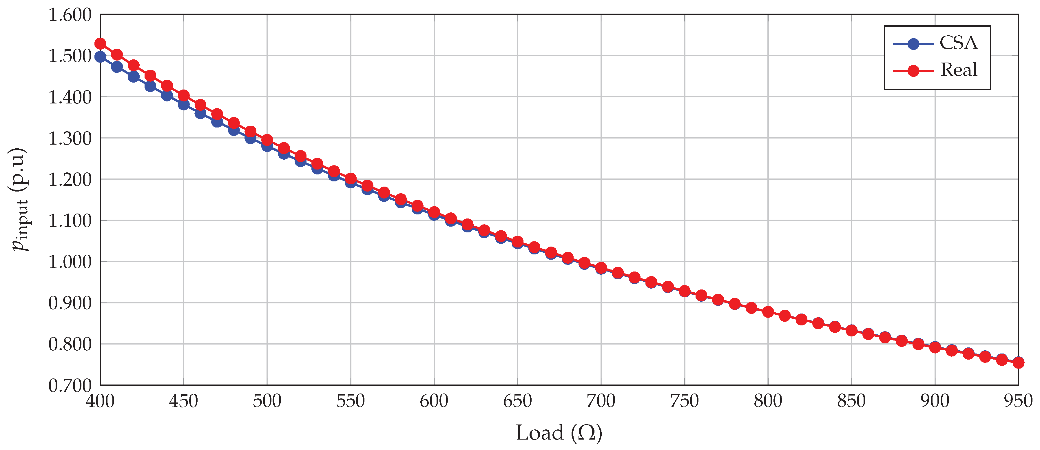
This work dealt with the proposition of the application of the CSA to the problem of the parametric estimation in single-phase transformers using voltage and current measures in their terminals. Numerical comparisons with the fmincon solver from MATLAB and the real data for the transformers reported in the current literature demonstrated that the CSA finds the best near-optimal values with minimum computational effort. Regarding the maximum estimation errors between the real data when compared with the CSA and the fmincon solutions, we found that in the case of our proposed method, these errors were 4.87%, 4.38%, and 6.00% for the 20 kVA, 45 kVA, and 112.5 kVA, respectively; while the fmincon found errors about 13.09%, 10.59%, and 7.86%, respectively. The CSA also arrived at better results in the case of the objective function estimation, when compared with the fmincon solver. The maximum estimation error in the case of the CSA was $5.14\times {10}^{-4}\%$, while it was $1.03\times {10}^{-3}\%$ for the comparative method, both in the case of the 20 kVA transformer, which confirmed the efficiency of the proposed optimization approach to estimate parameters in single-phase transformers.

The effectiveness and robustness of the proposed CSA were supported by the proposed parametrization of this algorithm. This allowed finding the best compromise with respect to the objective function minimization and the required processing times to solve the problem. The selected parameters took the following values: $A_f=0.80$, $t_{max}=50$; $N_e=50$; $N_i=25$. The main advantage of these parameters was that the expected execution time is approximately 1 s for all the test transformers analyzed.

Numerical comparisons regarding recently developed approaches in the current literature showed that in the case of exact methods, the proposed CSA finds the best objective function value, followed by the fmincon approach, and in case of metaheuristic optimizers, it was the sine–cosine algorithm.

Future works can be developed: (i) to extend the application of the CSA to solve estimation problems in rotative machines such as induction, synchronous, and direct current motors/generators; (ii) to verify the efficiency of the proposed CSA with experimental validations in distribution transformers.

References

1. García, J.D.M.; Jimenez, J.D.M.; Quintero, S.X.C. Implementation of an Energy Management System in Colombian Manufacturing—A Methodological Approach. Trans. Energy Syst. Eng. Appl. 2021, 2, 9–14. [Google Scholar] [CrossRef]
2. Guarín, S.; Velarde, S.; Castaño, E.; Molina-Cabrera, A. Construction and Simulation of a Planar Transformer Prototype. Trans. Energy Syst. Eng. Appl. 2021, 2, 1–7. [Google Scholar] [CrossRef]
3. Echeverri, M.G.; Rendón, R.A.G.; Lezama, J.M.L. Optimal Phase Balancing Planning for Loss Reduction in Distribution Systems using a Specialized Genetic Algorithm. Ing. Cienc. 2012, 8, 121–140. [Google Scholar] [CrossRef] [Green Version]
4. Bocanegra, S.Y.; Montoya, O.D.; Molina-Cabrera, A. Sine-cosine optimization approach applied to the parametric estimation in single-phase transformers by considering voltage and current measures. Dyna 2021, 88, 19–27. [Google Scholar] [CrossRef]
5. Biçen, Y.; Aras, F. Loadability of power transformer under regional climate conditions: The case of Turkey. Electr. Eng. 2014, 96, 347–358. [Google Scholar] [CrossRef]
6. Al-Badi, A.H.; Elmoudi, A.; Metwally, I.; Al-Wahaibi, A.; Al-Ajmi, H.; Al Bulushi, M. Losses reduction in distribution transformers. In Proceedings of the International Multi Conference of Engineers and Computer Scientists, Hong Kong, China, 16–18 March 2011; Volume 2, pp. 948–952. [Google Scholar]
7. Cortés-Caicedo, B.; Avellaneda-Gómez, L.S.; Montoya, O.D.; Alvarado-Barrios, L.; Chamorro, H.R. Application of the Vortex Search Algorithm to the Phase-Balancing Problem in Distribution Systems. Energies 2021, 14, 1282. [Google Scholar] [CrossRef]
8. Bocanegra, S.Y.; Montoya, O.D.; Molina-Cabrera, A. Parameter estimation in singe-phase transformers employing voltage and current measures (In Spanish). Rev. UIS Ing. 2020, 19, 63–75. [Google Scholar] [CrossRef]
9. Mgunda, M.C. Optimization of Power Transformer Design: Losses, Voltage Regulation and Tests. J. Power Energy Eng. 2017, 5, 45–74. [Google Scholar] [CrossRef] [Green Version]
10. Illias, H.; Mou, K.; Bakar, A. Estimation of transformer parameters from nameplate data by imperialist competitive and gravitational search algorithms. Swarm Evol. Comput. 2017, 36, 18–26. [Google Scholar] [CrossRef]
11. Icontec. NTC-3445 Transformadores Trifásicos Autorefrigerados, Tipo Seco Abierto y Encapsulado en Resina, Corriente sin Carga, Pérdidas y Tensión de Cortocircuito; Bogotá, Colombia, 1992; Available online: https://docplayer.es/23962496-Norma-tecnica-ntc-colombiana-3445.html (accessed on 12 October 2012).
12. Chapman, S. Electric Machinery Fundamentals; McGraw-Hill Series in Electrical and Computer Engineering; McGraw-Hill Companies: New York, NY, USA, 2005. [Google Scholar]
13. Ćalasan, M.; Mujičić, D.; Rubežić, V.; Radulović, M. Estimation of Equivalent Circuit Parameters of Single-Phase Transformer by Using Chaotic Optimization Approach. Energies 2019, 12, 1697. [Google Scholar] [CrossRef] [Green Version]
14. Zhang, Z.; Kang, N.; Mousavi, M.J. Real-time transformer parameter estimation using terminal measurements. In Proceedings of the 2015 IEEE Power & Energy Society General Meeting, Denver, CO, USA, 26–30 July 2015. [Google Scholar] [CrossRef]
15. Feyzi, M.; Sabahi, M. Online Dynamic Parameter Estimation of Transformer Equivalent Circuit. In Proceedings of the 2006 5th International Power Electronics and Motion Control Conference, Shanghai, China, 14–16 August 2006. [Google Scholar] [CrossRef]
16. Krishan, R.; Mishra, A.K.; Rajpurohit, B.S. Real-time parameter estimation of single-phase transformer. In Proceedings of the 2016 IEEE 7th Power India International Conference (PIICON), Bikaner, India, 25–27 November 2016. [Google Scholar] [CrossRef]
17. Arenas-Acuña, C.A.; Rodriguez-Contreras, J.A.; Montoya, O.D.; Rivas-Trujillo, E. Black-Hole Optimization Applied to the Parametric Estimation in Distribution Transformers Considering Voltage and Current Measures. Computers 2021, 10, 124. [Google Scholar] [CrossRef]
18. Mossad, M.I.; Azab, M.; Abu-Siada, A. Transformer Parameters Estimation From Nameplate Data Using Evolutionary Programming Techniques. IEEE Trans. Power Deliv. 2014, 29, 2118–2123. [Google Scholar] [CrossRef]
19. Abdelwanis, M.I.; Abaza, A.; El-Sehiemy, R.A.; Ibrahim, M.N.; Rezk, H. Parameter Estimation of Electric Power Transformers Using Coyote Optimization Algorithm With Experimental Verification. IEEE Access 2020, 8, 50036–50044. [Google Scholar] [CrossRef]
20. Calasan, M.; Jovanovic, A.; Rubezic, V.; Mujicic, D.; Deriszadeh, A. Notes on parameter estimation for single-phase transformer. IEEE Trans. Ind. Appl. 2020, 56, 3710–3718. [Google Scholar] [CrossRef]
21. Elsayed, S.K.; Agwa, A.M.; El-Dabbah, M.A.; Elattar, E.E. Slime Mold Optimizer for Transformer Parameters Identification with Experimental Validation. Intell. Autom. Soft Comput. 2021, 28, 639–651. [Google Scholar] [CrossRef]
22. Montoya, O.D.; Ramírez-Vanegas, C.A.; Grisales-Noreña, L.F. Parametric estimation in photovoltaic modules using the crow search algorithm. Int. J. Electr. Comput. Eng. 2022, 12, 82. [Google Scholar] [CrossRef]
23. Díaz, P.; Pérez-Cisneros, M.; Cuevas, E.; Avalos, O.; Gálvez, J.; Hinojosa, S.; Zaldivar, D. An Improved Crow Search Algorithm Applied to Energy Problems. Energies 2018, 11, 571. [Google Scholar] [CrossRef] [Green Version]
24. Cortés-Caicedo, B.; Avellaneda-Gómez, L.S.; Montoya, O.D.; Alvarado-Barrios, L.; Álvarez-Arroyo, C. An Improved Crow Search Algorithm Applied to the Phase Swapping Problem in Asymmetric Distribution Systems. Symmetry 2021, 13, 1329. [Google Scholar] [CrossRef]
25. Oliva, D.; Hinojosa, S.; Cuevas, E.; Pajares, G.; Avalos, O.; Gálvez, J. Cross entropy based thresholding for magnetic resonance brain images using Crow Search Algorithm. Expert Syst. Appl. 2017, 79, 164–180. [Google Scholar] [CrossRef]
26. Hussien, A.G.; Amin, M.; Wang, M.; Liang, G.; Alsanad, A.; Gumaei, A.; Chen, H. Crow Search Algorithm: Theory, Recent Advances, and Applications. IEEE Access 2020, 8, 173548–173565. [Google Scholar] [CrossRef]
27. Chaudhary, A.; Agarwal, A.P.; Rana, A.; Kumar, V. Crow Search Optimization Based Approach for Parameter Estimation of SRGMs. In Proceedings of the 2019 Amity International Conference on Artificial Intelligence (AICAI), Dubai, United Arab Emirates, 4–6 February 2019. [Google Scholar] [CrossRef]
28. Shirke, S.; Udayakumar, R. Evaluation of Crow Search Algorithm (CSA) for Optimization in Discrete Applications. In Proceedings of the 2019 3rd International Conference on Trends in Electronics and Informatics (ICOEI), Tirunelveli, India, 23–25 April 2019. [Google Scholar] [CrossRef]
Figure 1. Equivalent circuit for a single-phase transformer.
Computers 11 00009 g001
Figure 2. Equivalent reduced model of a single-phase transformer.
Computers 11 00009 g002
Figure 3. Crow’s movements: (a) from its initial position, the ith crow tries to follow the jth crow to know its food location; (b) at the final position, crow i has stolen the food of crow j [26].
Computers 11 00009 g003
Figure 4. Application of CSA to the studied problem.
Computers 11 00009 g004
Figure 5. Parametrization of the CSA using multiple tests with different setting parameters.
Computers 11 00009 g005
Figure 6. Comparative results between the real data and the values obtained with the CSA for the first test transformer.
Computers 11 00009 g006
Figure 7. Comparative results between the real data and the values obtained with the CSA for the second test transformer.
Computers 11 00009 g007
Figure 8. Comparative results between the real data and the values obtained with the CSA for the third test transformer.
Computers 11 00009 g008
Figure 9. Input power behavior for the fourth test system.
Computers 11 00009 g009