Author Contributions
Conceptualization, Y.Y. and J.C.; Methodology, Y.Y. and J.C.; Software, X.G.; Validation, Y.Y., X.G., M.X., L.Y. and J.C.; Formal analysis, Y.Y.; Investigation, Y.Y., M.X. and L.Y.; Resources, J.C., M.X. and L.Y.; Data curation, Y.Y.; Writing—original draft preparation, Y.Y.; Writing—review and editing, J.C.; Visualization, Y.Y.; Supervision, J.C.; Project administration, J.C.; Funding acquisition, J.C. All authors have read and agreed to the published version of the manuscript.
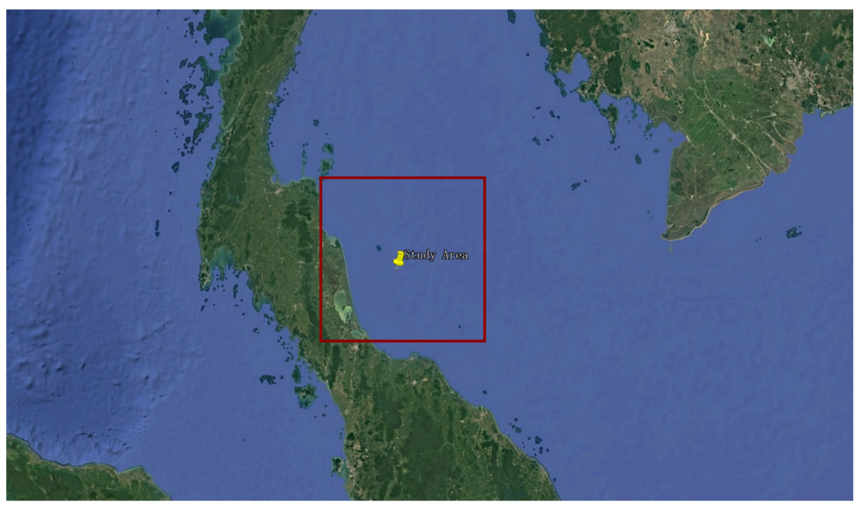
Figure 1.
Satellite imagery from Google Earth showing the location of the study site. The study area is delineated by the red box, and its approximate geographic center is indicated by the yellow pushpin.
Figure 1.
Satellite imagery from Google Earth showing the location of the study site. The study area is delineated by the red box, and its approximate geographic center is indicated by the yellow pushpin.
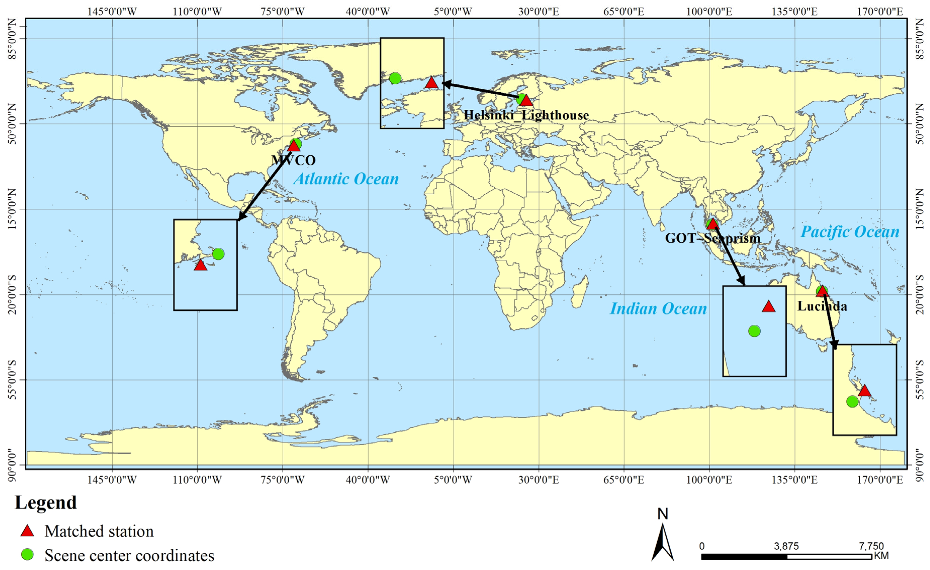
Figure 2.
Geographic locations of the four AERONET-OC validation sites and the corresponding centers of the remote sensing images used in this study. The black arrow indicates north, and the black box represents the scale bar.
Figure 2.
Geographic locations of the four AERONET-OC validation sites and the corresponding centers of the remote sensing images used in this study. The black arrow indicates north, and the black box represents the scale bar.
Figure 3.
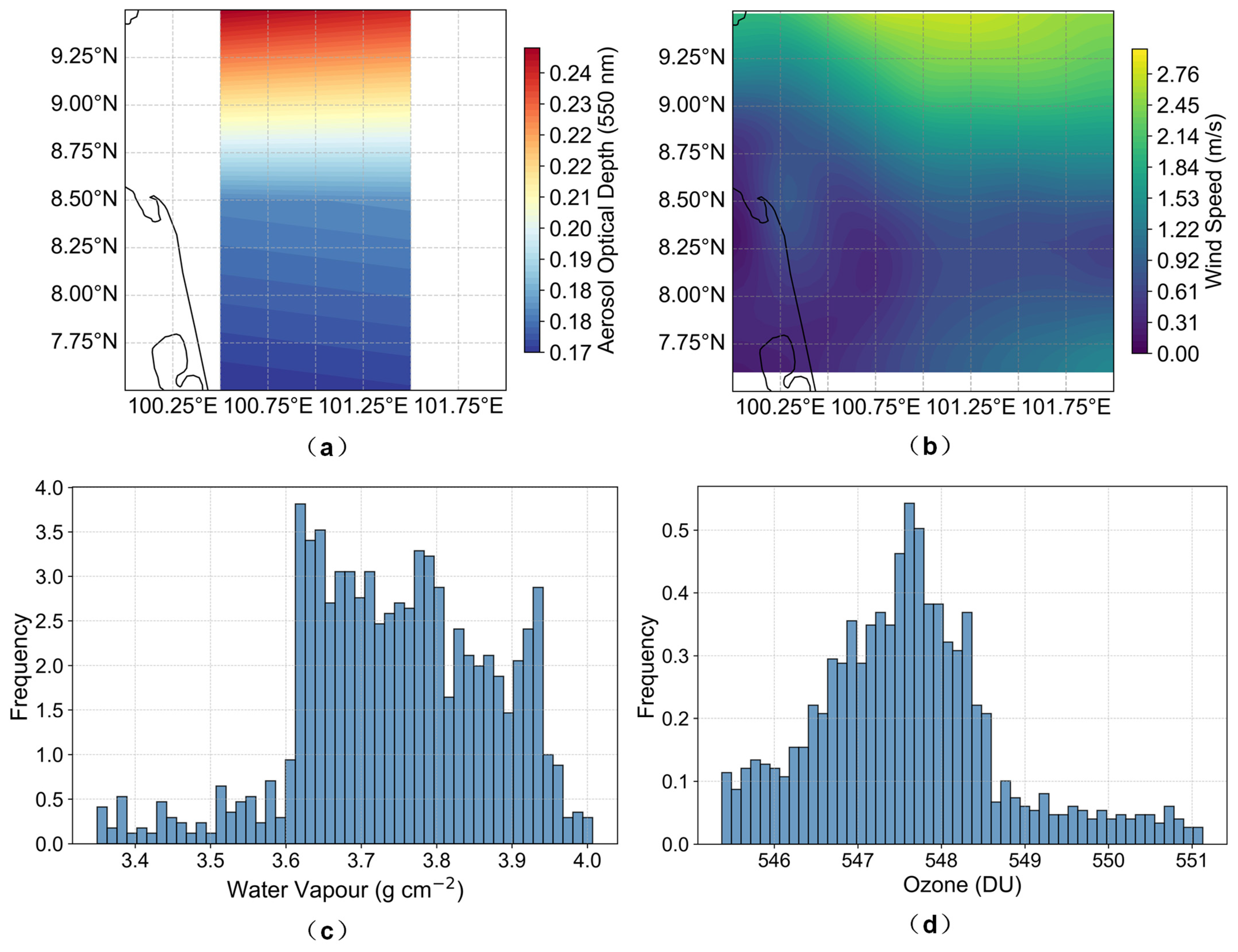
Spatial and statistical distributions of atmospheric parameters over the study area on 15 December 2015: (a) AOD, (b) wind speed, (c) water vapor frequency distribution, and (d) ozone frequency distribution. The curves in (a,b) indicate background geographic features.
Figure 3.
Spatial and statistical distributions of atmospheric parameters over the study area on 15 December 2015: (a) AOD, (b) wind speed, (c) water vapor frequency distribution, and (d) ozone frequency distribution. The curves in (a,b) indicate background geographic features.
Figure 4.
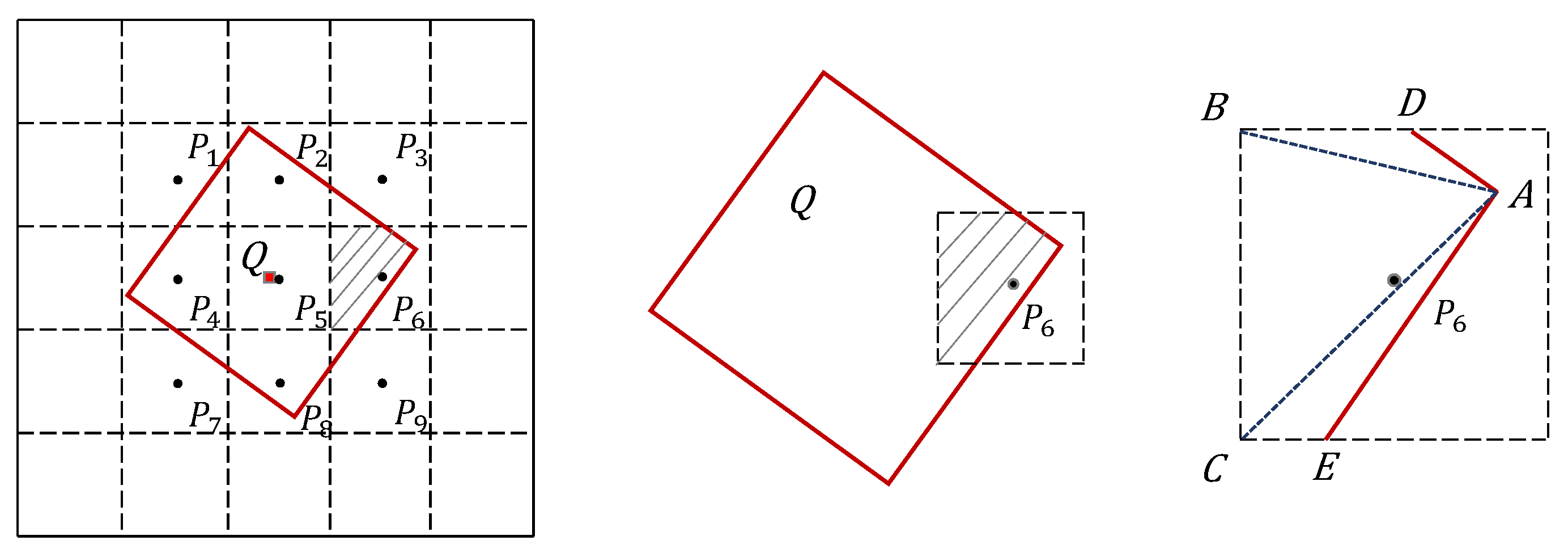
Principle of flux-conserving resampling. The overlap between source pixels and target pixel is computed using polygon clipping, and contributions are accumulated in an area-weighted manner.
Figure 4.
Principle of flux-conserving resampling. The overlap between source pixels and target pixel is computed using polygon clipping, and contributions are accumulated in an area-weighted manner.
Figure 5.
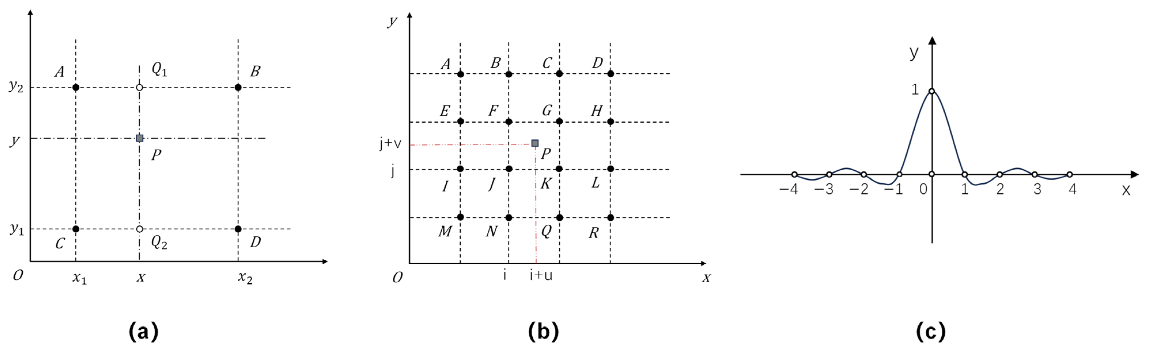
Schematic of three resampling methods: (a) bilinear interpolation, (b) cubic convolution interpolation, and (c) Lanczos kernel (a = 4).
Figure 5.
Schematic of three resampling methods: (a) bilinear interpolation, (b) cubic convolution interpolation, and (c) Lanczos kernel (a = 4).
Figure 6.
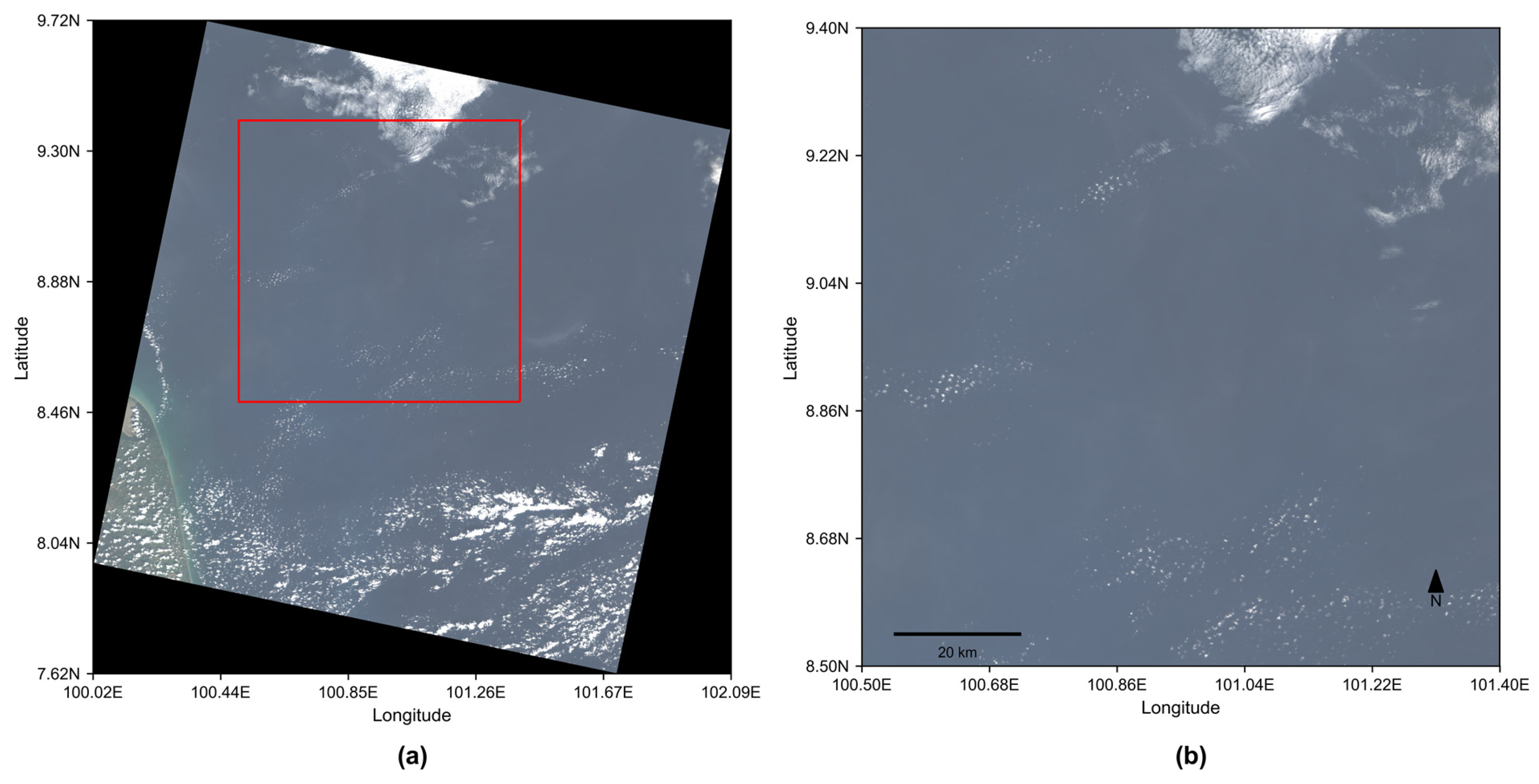
Calibration site selection results based on Landsat-8 RGB composites. (a) Spatial distribution of 100 km × 100 km candidate windows meeting the selection criteria. (b) Enlarged RGB view of the retained calibration region.
Figure 6.
Calibration site selection results based on Landsat-8 RGB composites. (a) Spatial distribution of 100 km × 100 km candidate windows meeting the selection criteria. (b) Enlarged RGB view of the retained calibration region.
Figure 7.
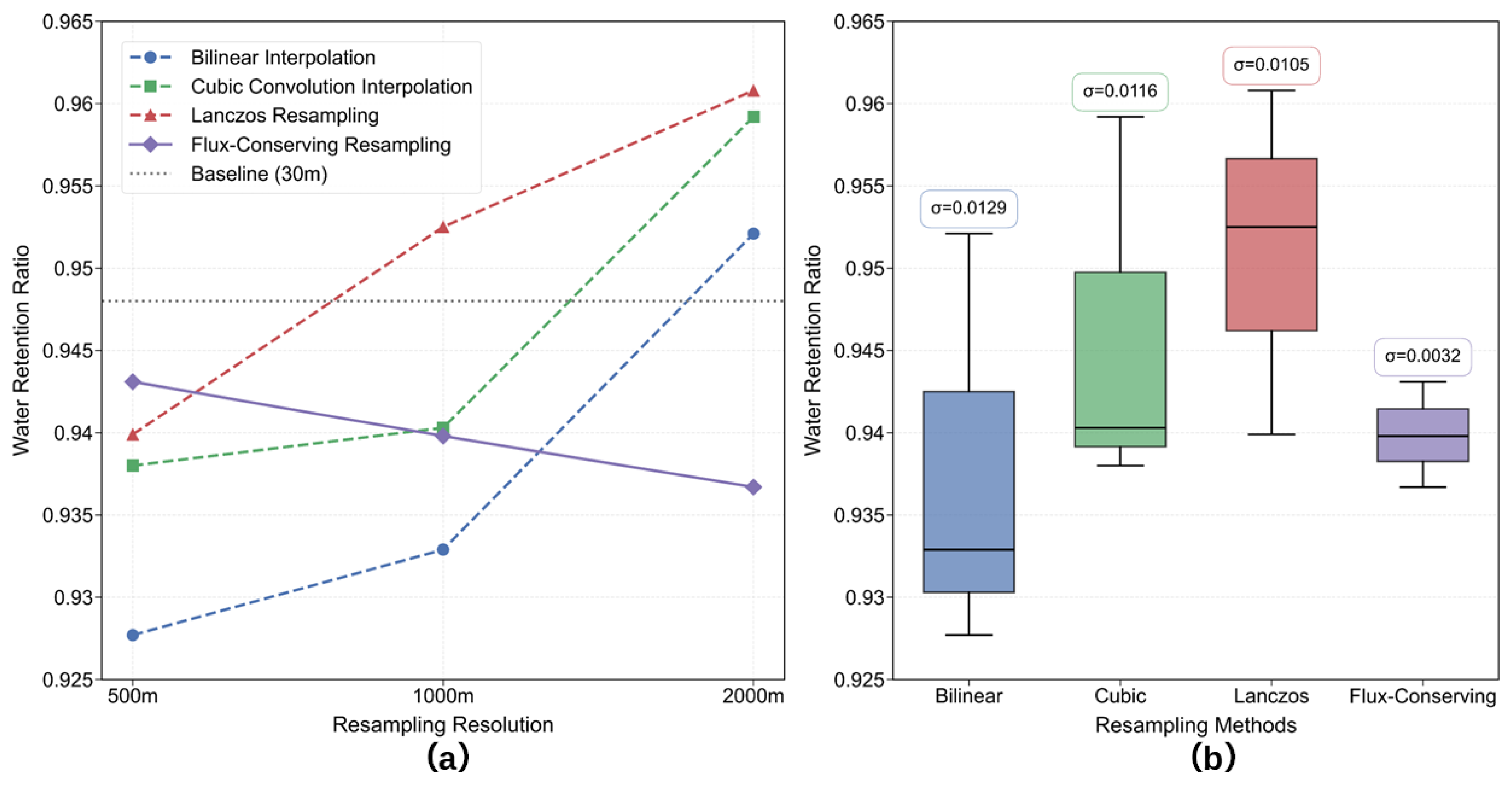
Performance evaluation of resampling methods for water pixel preservation across scales. (a) Water pixel preservation rates across spatial scales, (b) performance variability assessed through standard deviation (σ).
Figure 7.
Performance evaluation of resampling methods for water pixel preservation across scales. (a) Water pixel preservation rates across spatial scales, (b) performance variability assessed through standard deviation (σ).
Figure 8.
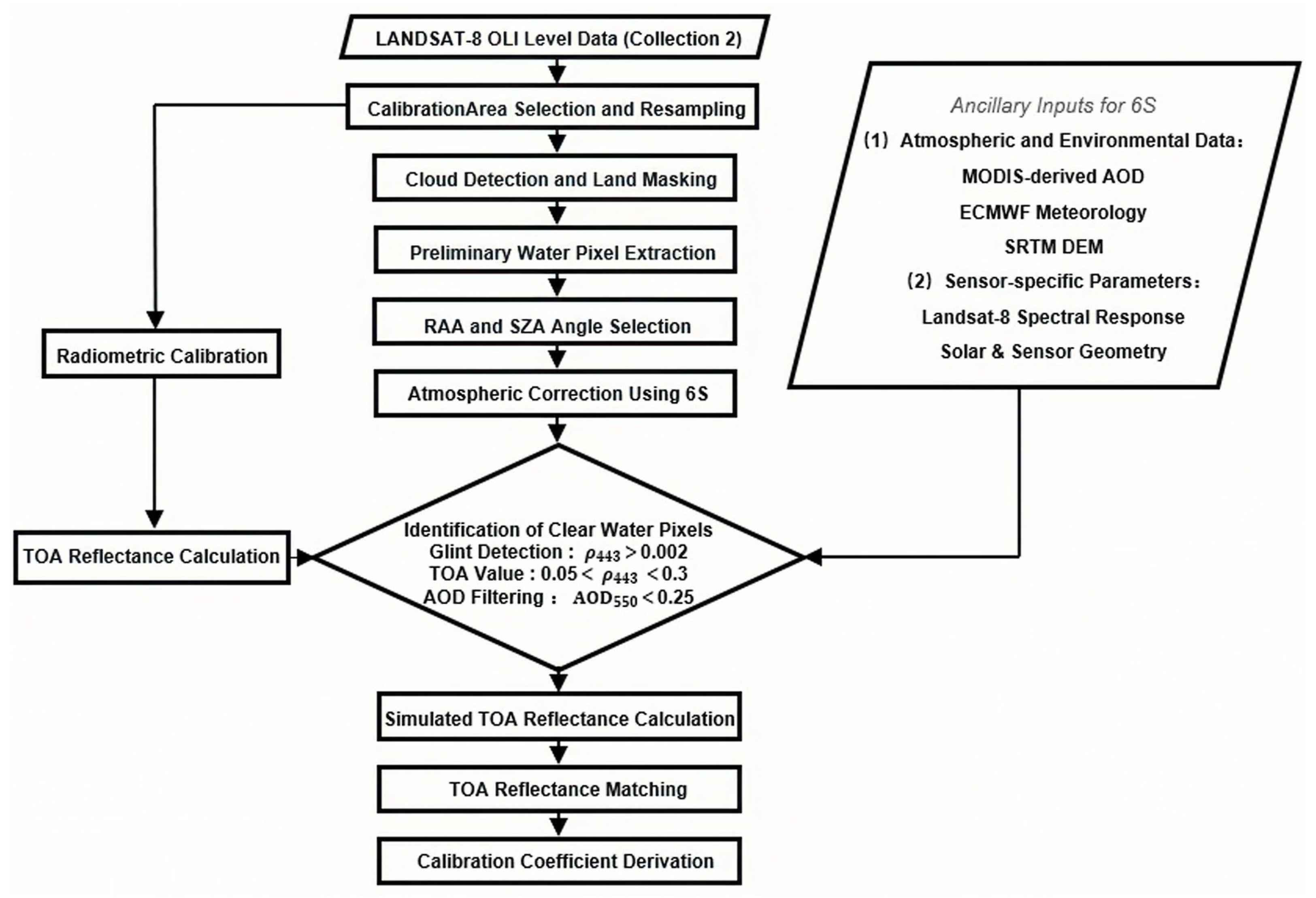
Schematic workflow for deriving the Rayleigh scattering calibration coefficient illustrating the processing chain from Landsat-8 OLI data input to final calibrated outputs.
Figure 8.
Schematic workflow for deriving the Rayleigh scattering calibration coefficient illustrating the processing chain from Landsat-8 OLI data input to final calibrated outputs.
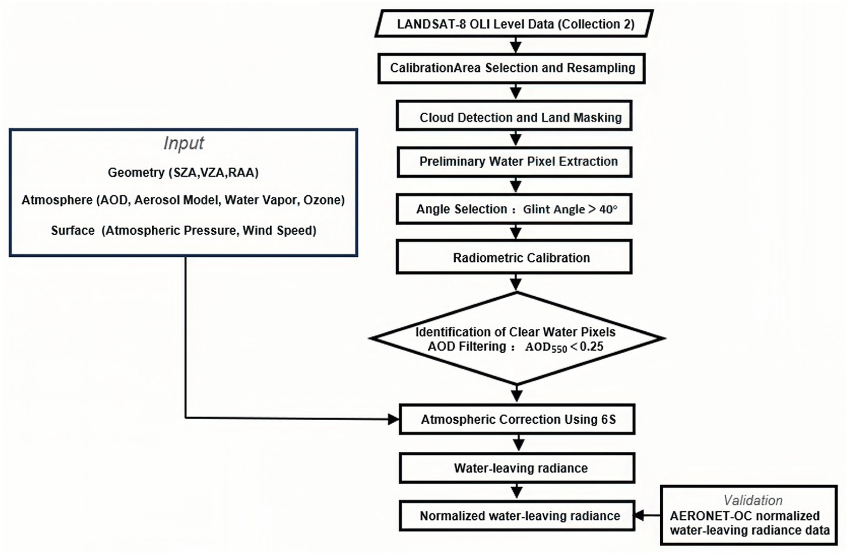
Figure 9.
Workflow for retrieving normalized water-leaving radiance from Landsat-8 OLI, including cloud-free water screening, 6S-based radiometric calibration and atmospheric correction, and validation with AERONET-OC data.
Figure 9.
Workflow for retrieving normalized water-leaving radiance from Landsat-8 OLI, including cloud-free water screening, 6S-based radiometric calibration and atmospheric correction, and validation with AERONET-OC data.
Figure 10.
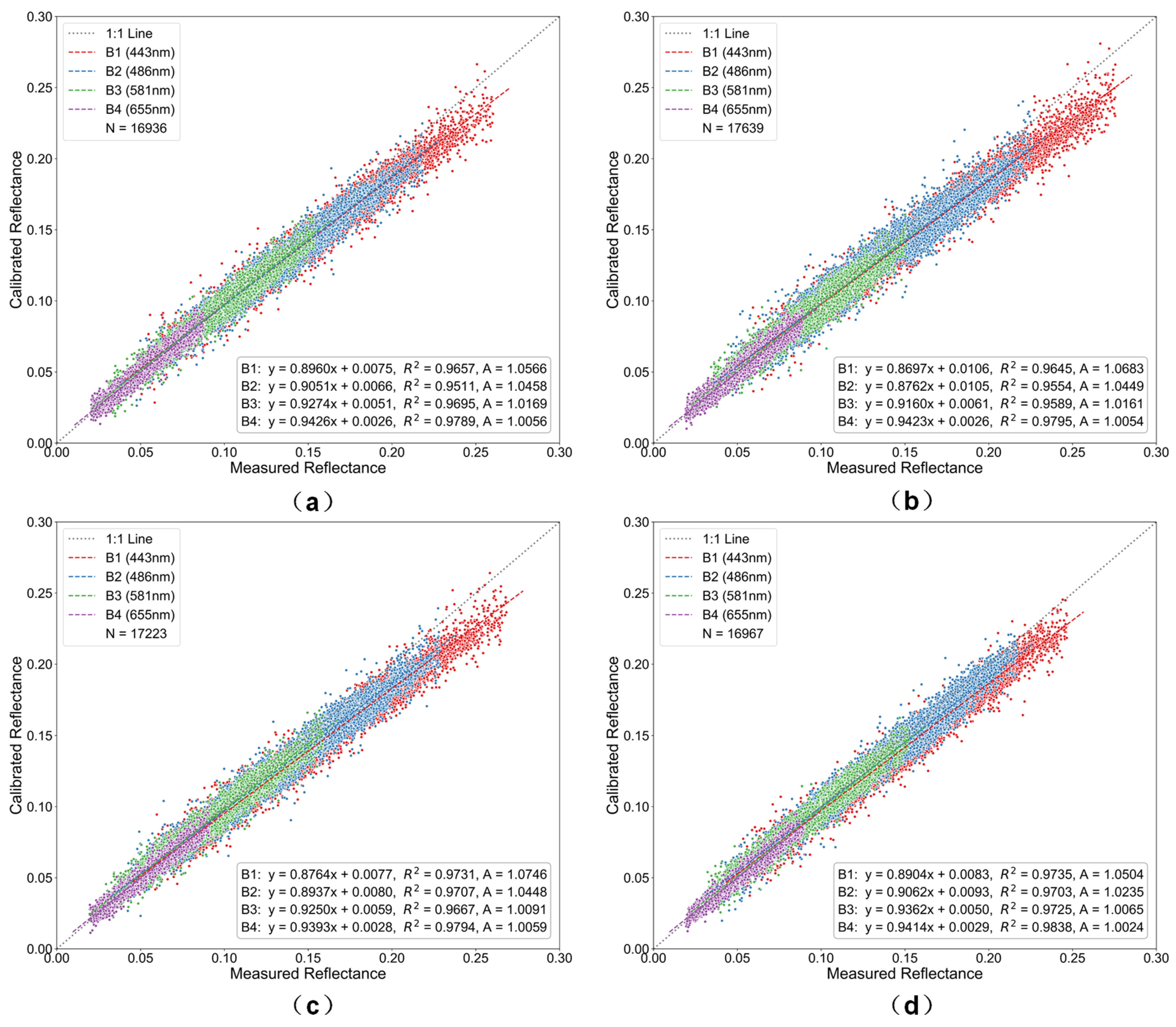
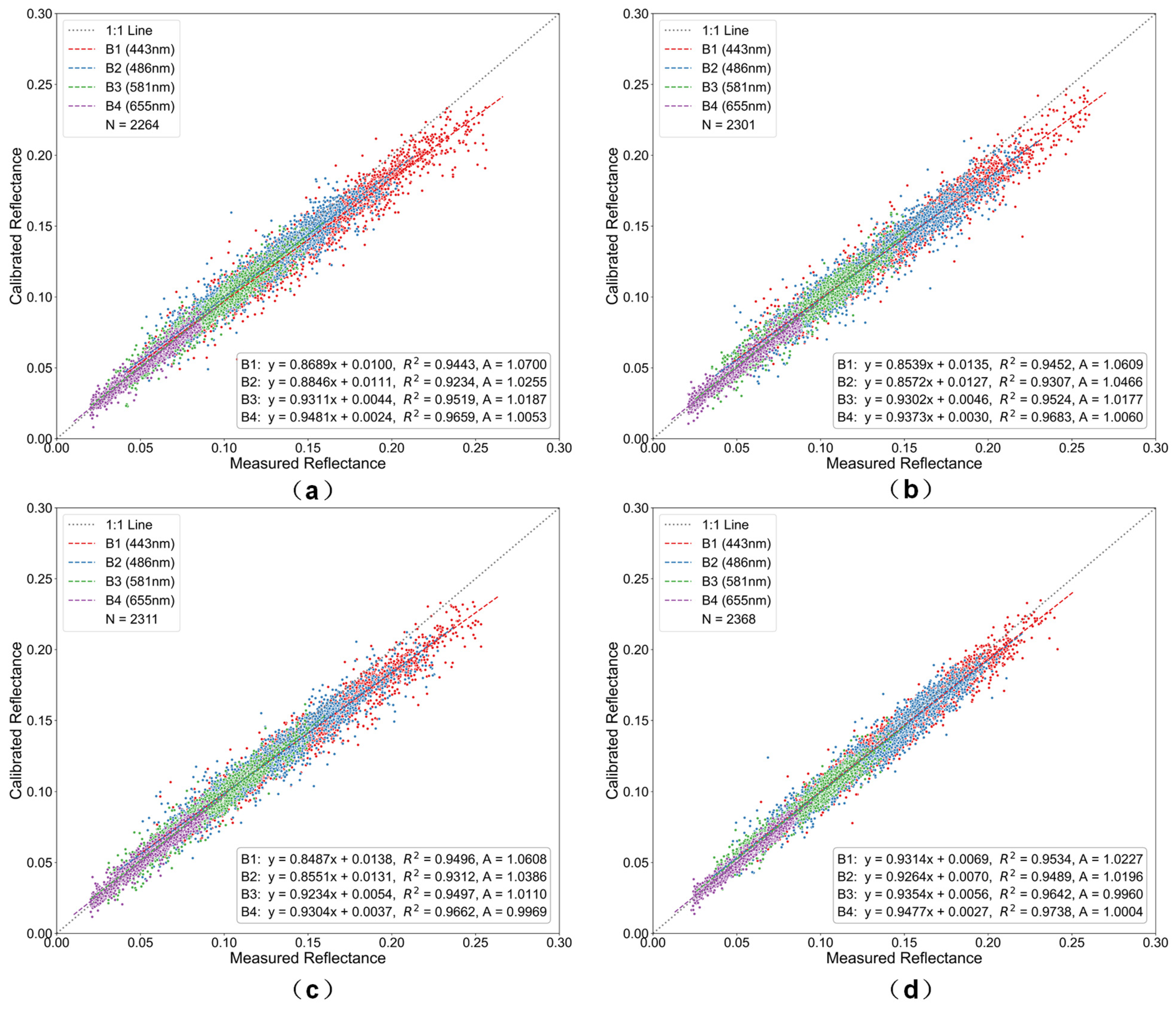
Scatter plots of radiometric calibration results at 500 m resolution for the four visible bands using different resampling methods: (a) bilinear, (b) cubic convolution, (c) Lanczos, and (d) flux-conserving. Colors denote the four spectral bands (blue for Band 1, green for Band 2, red for Band 3, and purple for Band 4).
Figure 10.
Scatter plots of radiometric calibration results at 500 m resolution for the four visible bands using different resampling methods: (a) bilinear, (b) cubic convolution, (c) Lanczos, and (d) flux-conserving. Colors denote the four spectral bands (blue for Band 1, green for Band 2, red for Band 3, and purple for Band 4).
Figure 11.
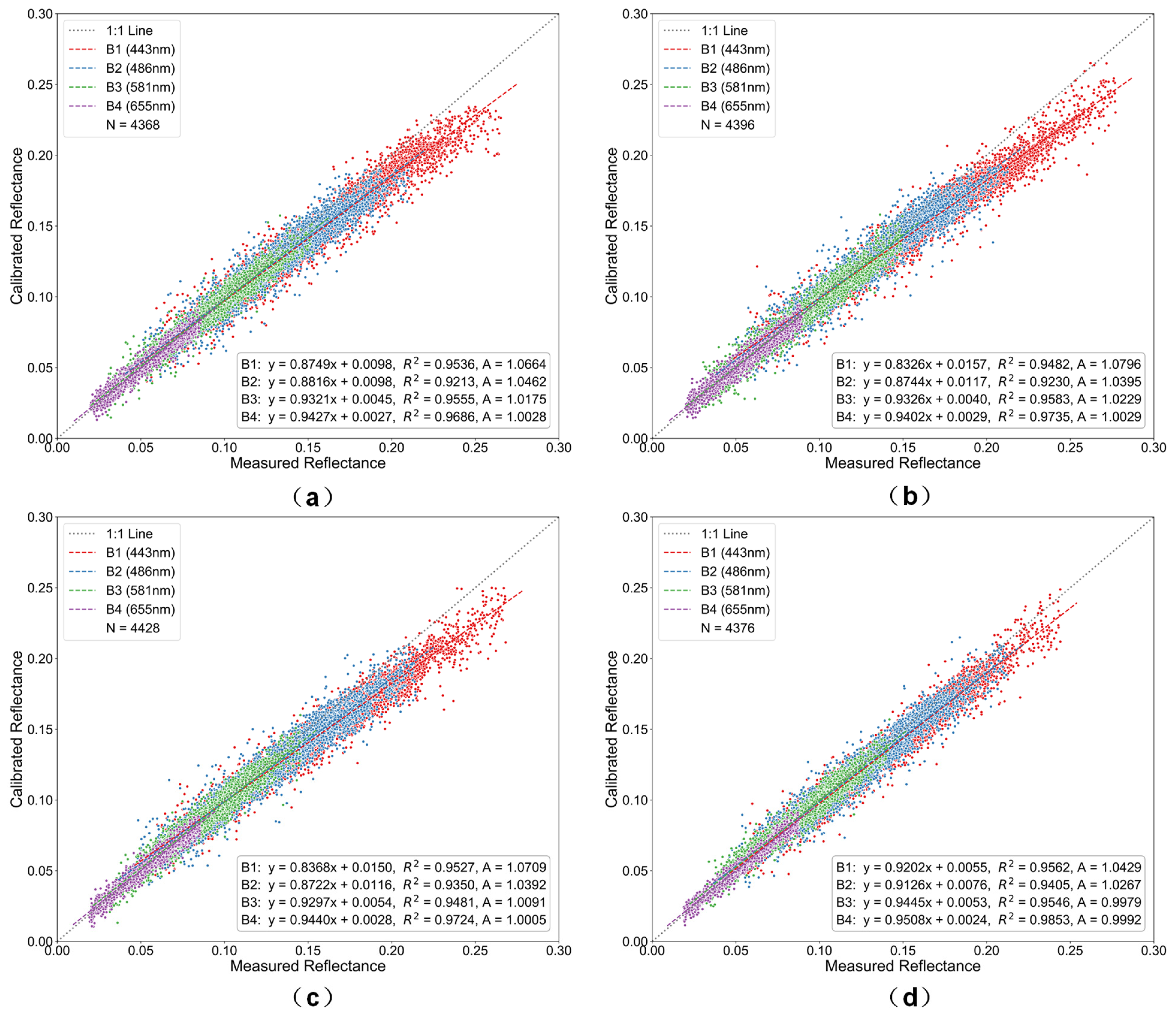
Scatter plots of radiometric calibration results at 1000 m resolution for the four visible bands using different resampling methods: (a) bilinear, (b) cubic convolution, (c) Lanczos, and (d) flux-conserving. Colors denote the four spectral bands (blue for Band 1, green for Band 2, red for Band 3, and purple for Band 4).
Figure 11.
Scatter plots of radiometric calibration results at 1000 m resolution for the four visible bands using different resampling methods: (a) bilinear, (b) cubic convolution, (c) Lanczos, and (d) flux-conserving. Colors denote the four spectral bands (blue for Band 1, green for Band 2, red for Band 3, and purple for Band 4).
Figure 12.
Scatter plots of radiometric calibration results at 2000 m resolution for the four visible bands using different resampling methods: (a) bilinear, (b) cubic convolution, (c) Lanczos, and (d) flux-conserving. Colors denote the four spectral bands (blue for Band 1, green for Band 2, red for Band 3, and purple for Band 4).
Figure 12.
Scatter plots of radiometric calibration results at 2000 m resolution for the four visible bands using different resampling methods: (a) bilinear, (b) cubic convolution, (c) Lanczos, and (d) flux-conserving. Colors denote the four spectral bands (blue for Band 1, green for Band 2, red for Band 3, and purple for Band 4).
Figure 13.
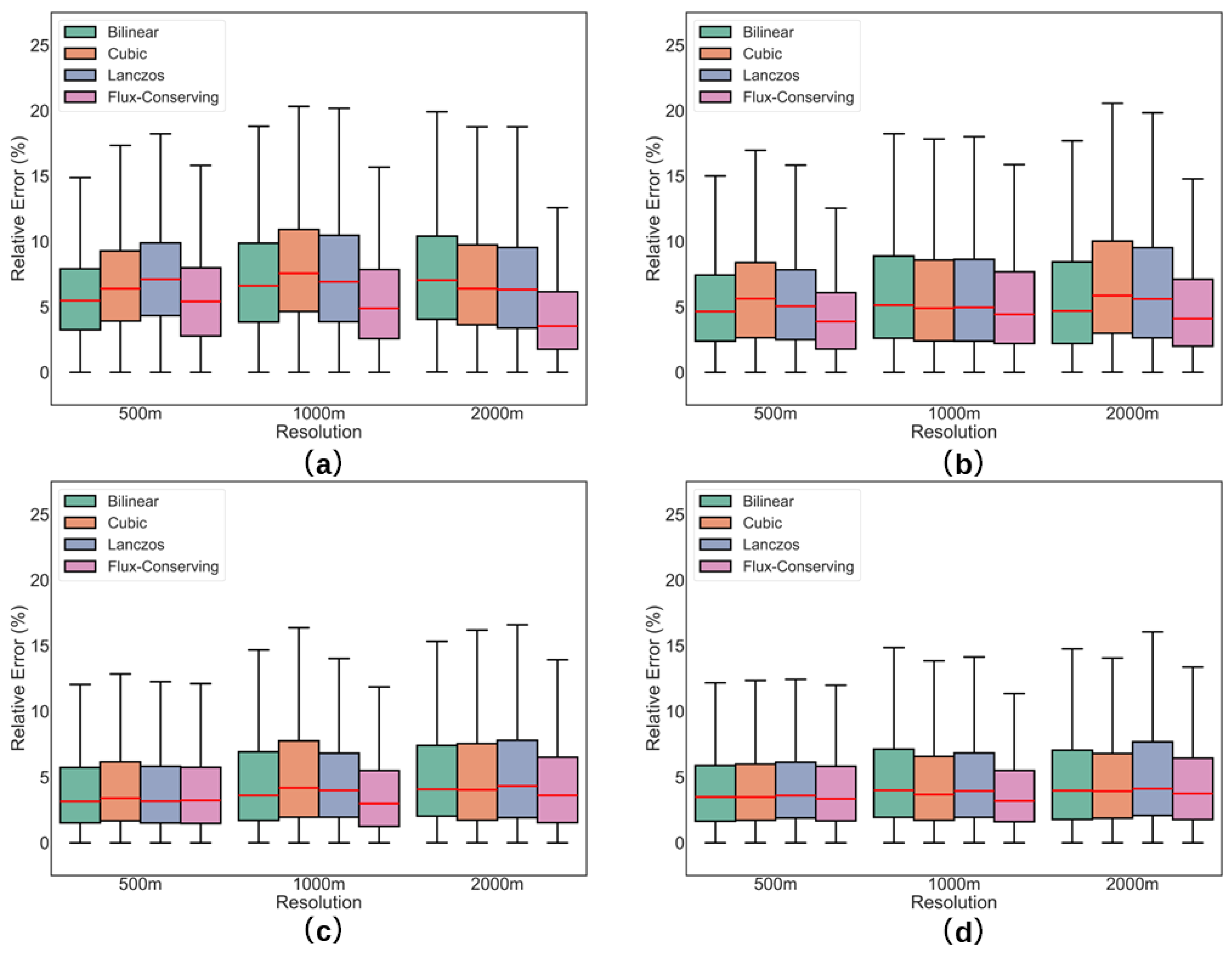
Relative errors of different resampling methods at spatial resolutions of 500 m, 1000 m, and 2000 m across the investigated spectral bands: (a) 443 nm, (b) 486 nm, (c) 561 nm, and (d) 655 nm.
Figure 13.
Relative errors of different resampling methods at spatial resolutions of 500 m, 1000 m, and 2000 m across the investigated spectral bands: (a) 443 nm, (b) 486 nm, (c) 561 nm, and (d) 655 nm.
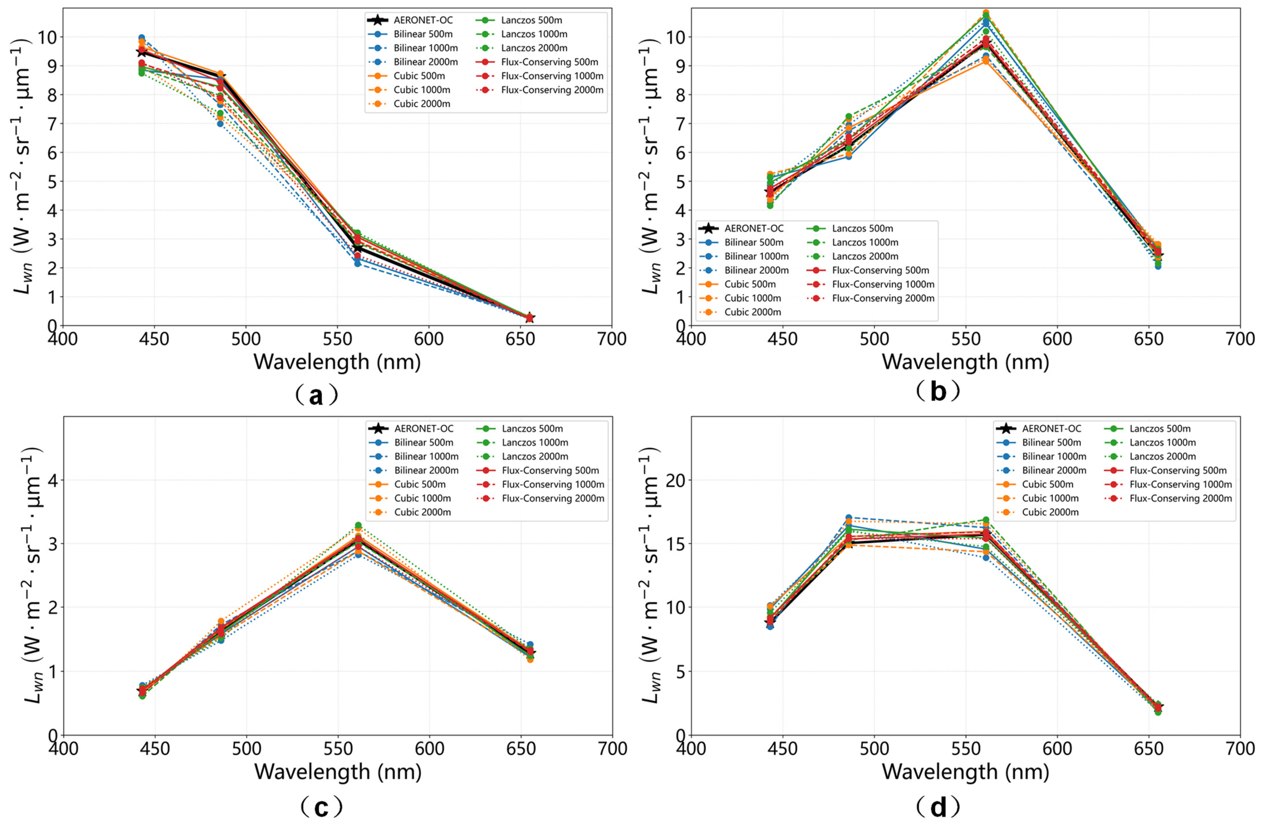
Figure 14.
Multi-site comparison of normalized water-leaving radiance retrieved using various resampling methods based on Level 1.5 data. (a) GOT-Seaprism site; (b) MVCO site; (c) Helsinki_Lighthouse site; (d) Lucinda site.
Figure 14.
Multi-site comparison of normalized water-leaving radiance retrieved using various resampling methods based on Level 1.5 data. (a) GOT-Seaprism site; (b) MVCO site; (c) Helsinki_Lighthouse site; (d) Lucinda site.
Table 1.
Spectral characteristics of Landsat-8 OLI bands 1.
Table 1.
Spectral characteristics of Landsat-8 OLI bands 1.
| Band Number | Band Name | Central Wavelength (nm) | Spatial Resolution (m) |
|---|
| 1 | Coastal/Aerosol | 443 | 30 |
| 2 | Blue | 486 | 30 |
| 3 | Green | 561 | 30 |
| 4 | Red | 655 | 30 |
| 5 | Near-infrared (NIR) | 865 | 30 |
| 6 | Shortwave infrared 1 (SWIR-1) | 1609 | 30 |
| 7 | Shortwave infrared 2 (SWIR-2) | 2201 | 30 |
| 8 | Panchromatic | 592 | 15 |
| 9 | Cirrus | 1373 | 30 |
Table 2.
Landsat-8 OLI scenes matched with AERONET-OC stations.
Table 2.
Landsat-8 OLI scenes matched with AERONET-OC stations.
| Acquisition Date (UTC) | Path/Row | Scene Center Coordinates | Cloud Cover (%) | Matched Station |
|---|
| 15 December 2015 | 128/54 | (8.67° N, 101.05° E) | 6.83 | GOT–Seaprism |
| 23 April 2018 | 11/31 | (41.75° N, 69.81° W) | 3.00 | MVCO |
| 28 June 2019 | 189/18 | (60.07° N, 23.09° E) | 3.50 | Helsinki_Lighthouse |
| 8 February 2021 | 95/73 | (18.79° S, 146.10° E) | 6.28 | Lucinda |
Table 3.
Input parameters for the LUT simulations.
Table 3.
Input parameters for the LUT simulations.
| Parameter (Unit) | Values | Interval |
|---|
| Central Wavelength (nm) | 443 nm, 486 nm, 561 nm, 655 nm | Fixed |
| Solar Zenith Angle (°) | 0~80° | 5° |
| Viewing Zenith Angle (°) | 0~7.5° | 1.5° |
| Relative Azimuth Angle (°) | 0~180° | 10° |
| Aerosol Optical Depth | 1 × 10⁻⁶~0.5 at 550 nm | 0.03 (AOD < 0.3)
0.05 (AOD ≥ 0.3) |
| Aerosol Model | Maritime | - |
| Wind Speed (m s−1) | 0~5 | 0.5 |
| Atmospheric Profile | Water Vapor Content (g cm−2) | 3.75 | Fixed |
| Ozone Concentration (DU) | 547.46 DU | Fixed |
Table 4.
Statistical comparison of relative errors (%) between observed and calibrated TOA radiance across different bands and spatial resolutions.
Table 4.
Statistical comparison of relative errors (%) between observed and calibrated TOA radiance across different bands and spatial resolutions.
| Band | Resolution | Average Relative Error/% | STD of Relative Error/% |
|---|
| BL | CC | Lanczos | FC | BL | CC | Lanczos | FC |
|---|
| 443 nm | 500 m | 5.90 | 6.74 | 7.30 | 5.71 | 3.79 | 3.95 | 4.07 | 3.77 |
| 1000 m | 7.37 | 8.12 | 7.52 | 5.70 | 5.07 | 5.06 | 4.92 | 4.36 |
| 2000 m | 7.80 | 7.17 | 6.93 | 4.36 | 5.31 | 5.20 | 4.86 | 3.59 |
| 486 nm | 500 m | 5.26 | 6.03 | 5.60 | 4.37 | 3.81 | 4.45 | 4.12 | 3.48 |
| 1000 m | 6.37 | 6.26 | 6.24 | 5.57 | 5.26 | 5.50 | 5.56 | 4.77 |
| 2000 m | 6.08 | 7.31 | 6.81 | 5.24 | 5.62 | 6.36 | 5.78 | 4.91 |
| 561 nm | 500 m | 4.12 | 4.56 | 4.15 | 4.17 | 3.75 | 4.38 | 3.86 | 3.91 |
| 1000 m | 5.07 | 5.74 | 5.08 | 4.16 | 5.25 | 5.79 | 4.60 | 4.45 |
| 2000 m | 5.51 | 5.58 | 5.75 | 4.78 | 5.25 | 5.66 | 5.76 | 4.64 |
| 655 nm | 500 m | 4.38 | 4.57 | 4.59 | 4.33 | 4.01 | 4.44 | 4.10 | 3.84 |
| 1000 m | 5.36 | 5.14 | 4.22 | 5.18 | 5.15 | 5.38 | 4.98 | 5.00 |
| 2000 m | 5.37 | 5.34 | 5.76 | 4.81 | 5.47 | 5.72 | 5.83 | 4.38 |
Table 5.
Optimal resampling method and relative error (%) of TOA radiance by site, spectral band, and spatial resolution.
Table 5.
Optimal resampling method and relative error (%) of TOA radiance by site, spectral band, and spatial resolution.
| Site | Resolution | Band |
|---|
| 443 nm | 486 nm | 561 nm | 655 nm |
|---|
| GOT-Seaprism | 500 m | FC (0.8%) | CC (1.2%) | FC (13.3%) | Lanczos (5.9%) |
| 1000 m | CC (3.8%) | FC (−4.8%) | Lanczos (6.3%) | Lanczos (8.1%) |
| 2000 m | FC (−3.9%) | FC (−8.6%) | FC (−10.0%) | FC (6.7%) |
| MVCO | 500 m | FC (2.6%) | FC (1.9%) | FC (0.6%) | Lanczos (1.2%) |
| 1000 m | FC (−1.7%) | FC (3.5%) | Lanczos (−1.4%) | CC (−2.9%) |
| 2000 m | FC (0.4%) | Lanczos (−1.3%) | FC (−0.7%) | FC (6.6%) |
| Helsinki_Lighthouse | 500 m | CC (−1.4%) | Lanczos (−1.2%) | FC (0.7%) | FC (2.3%) |
| 1000 m | FC (−4.3%) | FC (1.9%) | Lanczos (−1.0%) | FC (1.6%) |
| 2000 m | FC (5.8%) | FC (−2.5%) | FC (−3.3%) | FC (3.9%) |
| Lucinda | 500 m | Lanczos (3.8%) | FC (2.1%) | FC (0.3%) | Lanczos (−2.2%) |
| 1000 m | FC (0.7%) | CC (−1.0%) | FC (1.4%) | FC (0.9%) |
| 2000 m | CC (1.5%) | FC (2.4%) | FC (−2.0%) | FC (−5.8%) |
Table 6.
Atmospheric correction uncertainty contributions and combined uncertainty of TOA reflectance for different spectral bands.
Table 6.
Atmospheric correction uncertainty contributions and combined uncertainty of TOA reflectance for different spectral bands.
| Band (nm) | (%) | (%) | (%) |
|---|
| 443 | 1.08 | 1.66 | 1.98 |
| 486 | 1.05 | 1.39 | 1.74 |
| 561 | 0.83 | 1.01 | 1.31 |
| 655 | 0.67 | 0.93 | 1.15 |
Table 7.
Spatial resolution uncertainty of TOA reflectance for different spectral bands at 500 m, 1000 m, and 2000 m resolutions.
Table 7.
Spatial resolution uncertainty of TOA reflectance for different spectral bands at 500 m, 1000 m, and 2000 m resolutions.
| Band (nm) | (%) | (%) | (%)
|
|---|
| 443 | 1.82 | 3.05 | 5.12 |
| 486 | 1.57 | 2.91 | 4.69 |
| 561 | 1.41 | 2.36 | 3.94 |
| 655 | 1.09 | 2.08 | 3.32 |
Table 8.
Pixel-Level Water-Leaving Radiance Metrics for Flux-Conserving Resampling at Four Sites.
Table 8.
Pixel-Level Water-Leaving Radiance Metrics for Flux-Conserving Resampling at Four Sites.
| Site | Resolution (m) | RMSE | R2 |
|---|
| GOT-Seaprism | 500 m | 0.006 | 0.920 |
| 1000 m | 0.009 | 0.883 |
| 2000 m | 0.011 | 0.845 |
| MVCO | 500 m | 0.005 | 0.930 |
| 1000 m | 0.006 | 0.897 |
| 2000 m | 0.009 | 0.862 |
| Helsinki_Lighthouse | 500 m | 0.007 | 0.904 |
| 1000 m | 0.009 | 0.860 |
| 2000 m | 0.013 | 0.833 |
| Lucinda | 500 m | 0.004 | 0.952 |
| 1000 m | 0.005 | 0.926 |
| 2000 m | 0.008 | 0.889 |