Figure 1.
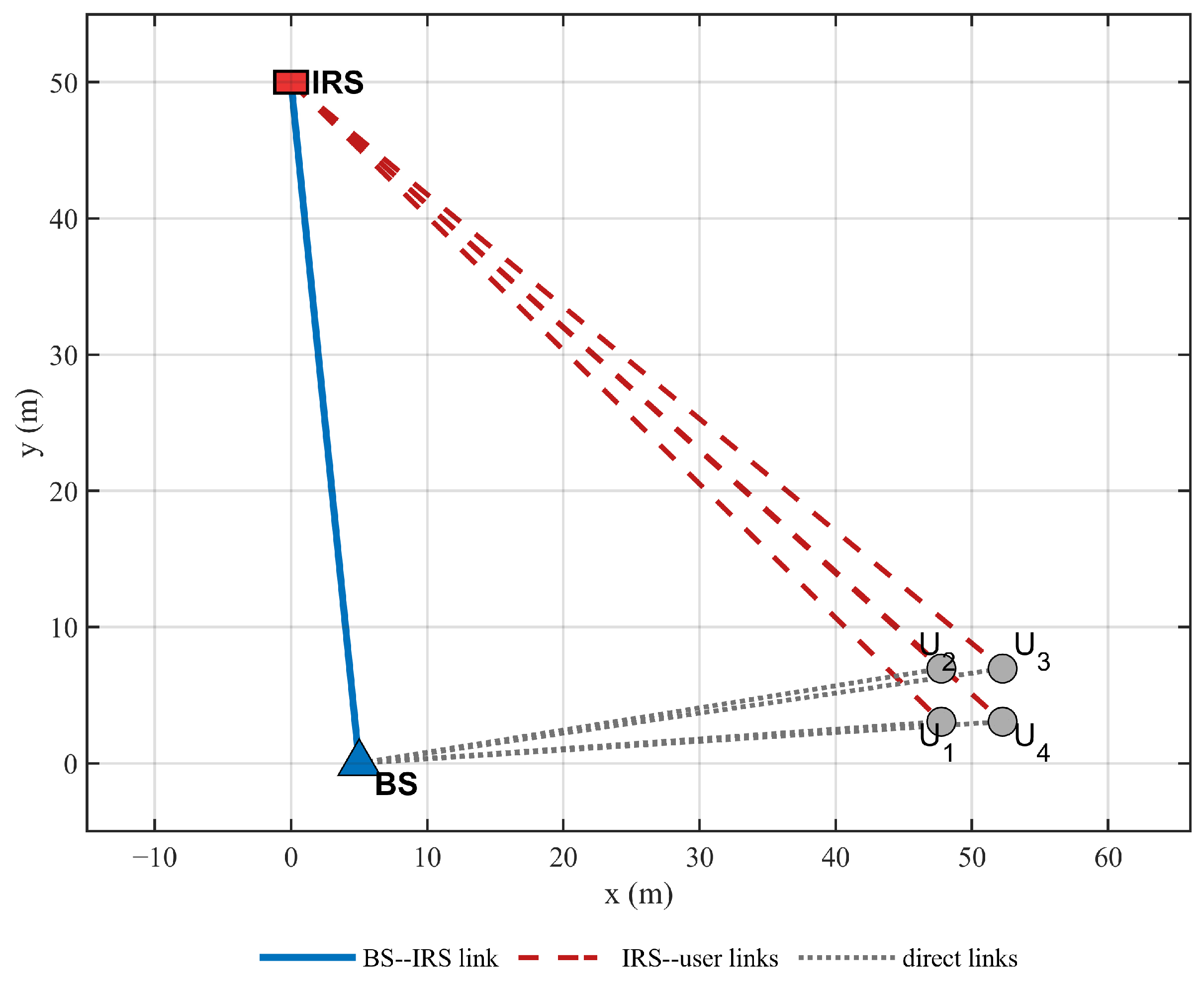
Top view of the simulated IRS-assisted NOMA downlink. The blue solid line denotes the BS–IRS link, the red dashed lines denote the IRS–user links, and the gray dotted lines denote the direct BS–user links. Together, the blue and red links form the two-hop BS–IRS–user paths.
Figure 1.
Top view of the simulated IRS-assisted NOMA downlink. The blue solid line denotes the BS–IRS link, the red dashed lines denote the IRS–user links, and the gray dotted lines denote the direct BS–user links. Together, the blue and red links form the two-hop BS–IRS–user paths.
Figure 2.
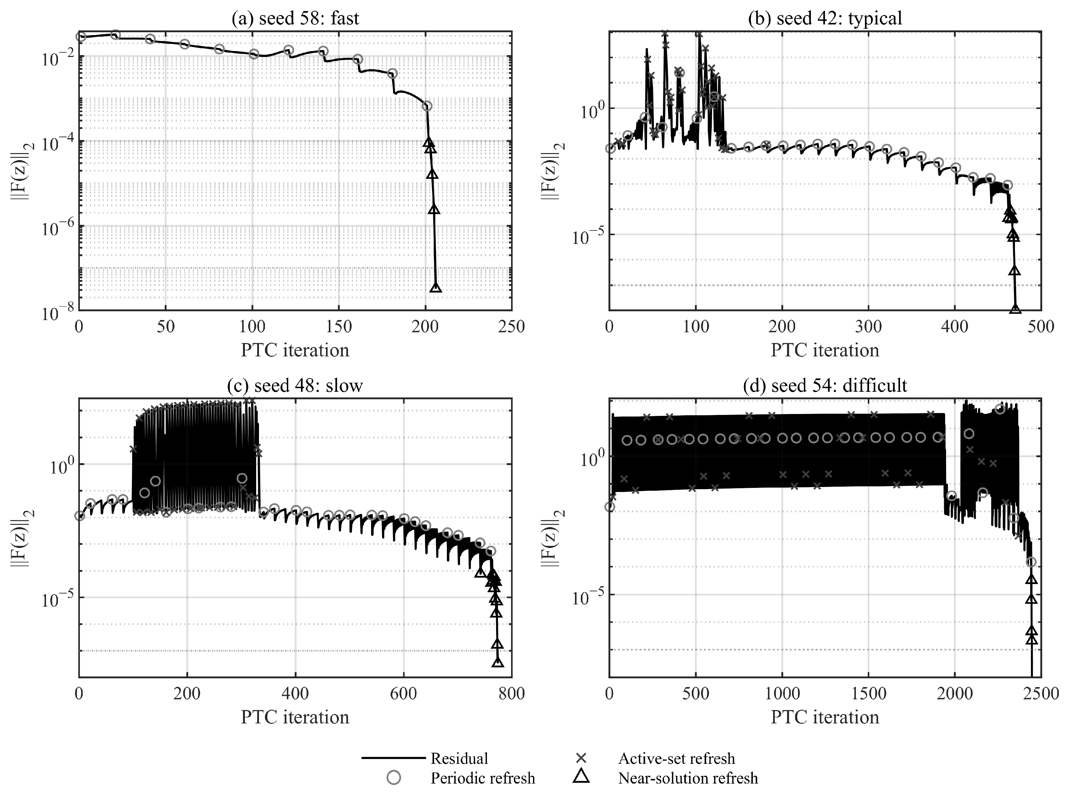
JODS-PD convergence for four representative channels. Panels (a–d) show the flow/KKT residual histories for seeds 58, 42, 48, and 54, respectively. Circles mark scheduled or periodic generalized Jacobian refreshes, crosses mark active-set-triggered refreshes, and triangles mark near-root refreshes. The nonmonotone middle phases correspond to accepted PTC branch transitions.
Figure 2.
JODS-PD convergence for four representative channels. Panels (a–d) show the flow/KKT residual histories for seeds 58, 42, 48, and 54, respectively. Circles mark scheduled or periodic generalized Jacobian refreshes, crosses mark active-set-triggered refreshes, and triangles mark near-root refreshes. The nonmonotone middle phases correspond to accepted PTC branch transitions.
Figure 3.
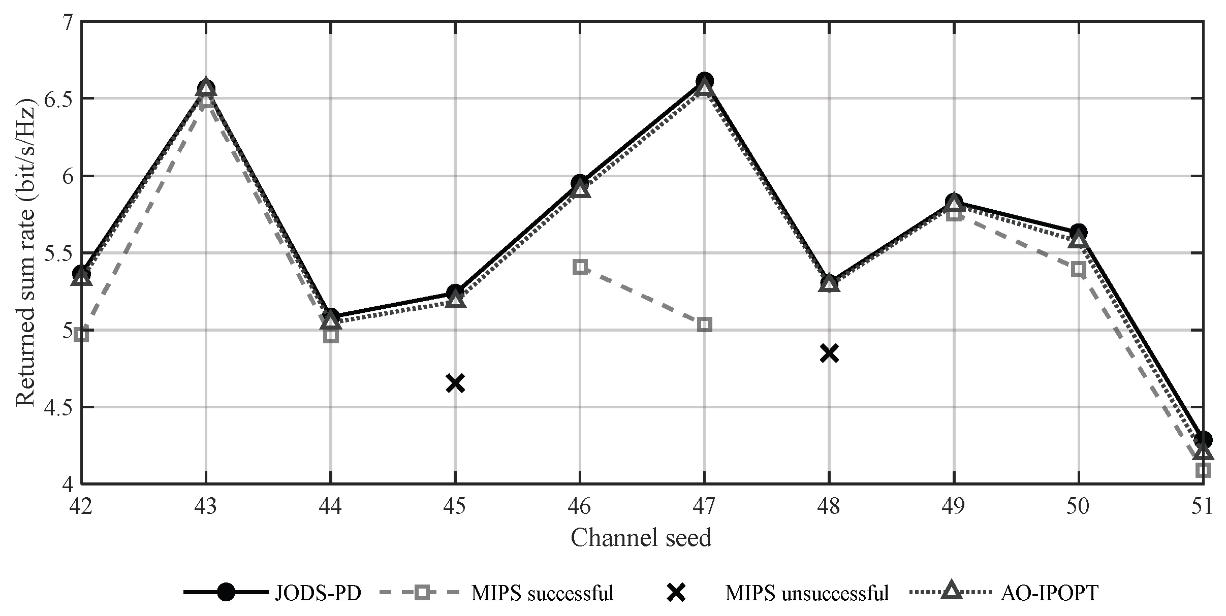
Per-seed returned sum rate for JODS-PD, AO-IPOPT, and MIPS on the matched benchmark channels. Open or missing MIPS markers identify endpoints that do not meet the common 10−6 primal feasibility criterion.
Figure 3.
Per-seed returned sum rate for JODS-PD, AO-IPOPT, and MIPS on the matched benchmark channels. Open or missing MIPS markers identify endpoints that do not meet the common 10−6 primal feasibility criterion.
Figure 4.
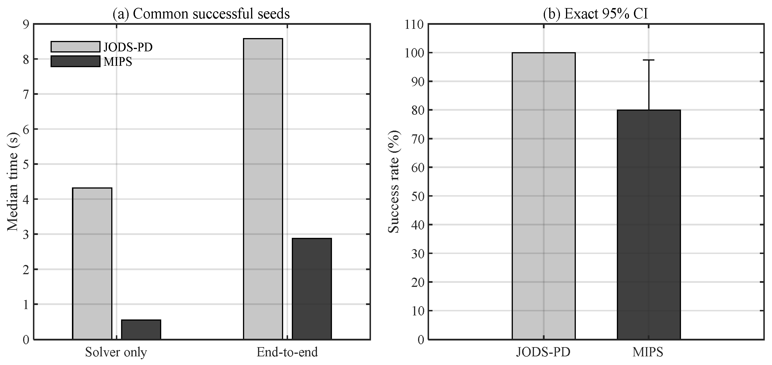
JODS-PD and MIPS reliability and timing. (a) Median solver-only and end-to-end wall times on eight common successes; (b) success rates with exact 95% binomial confidence intervals.
Figure 4.
JODS-PD and MIPS reliability and timing. (a) Median solver-only and end-to-end wall times on eight common successes; (b) success rates with exact 95% binomial confidence intervals.
Figure 5.
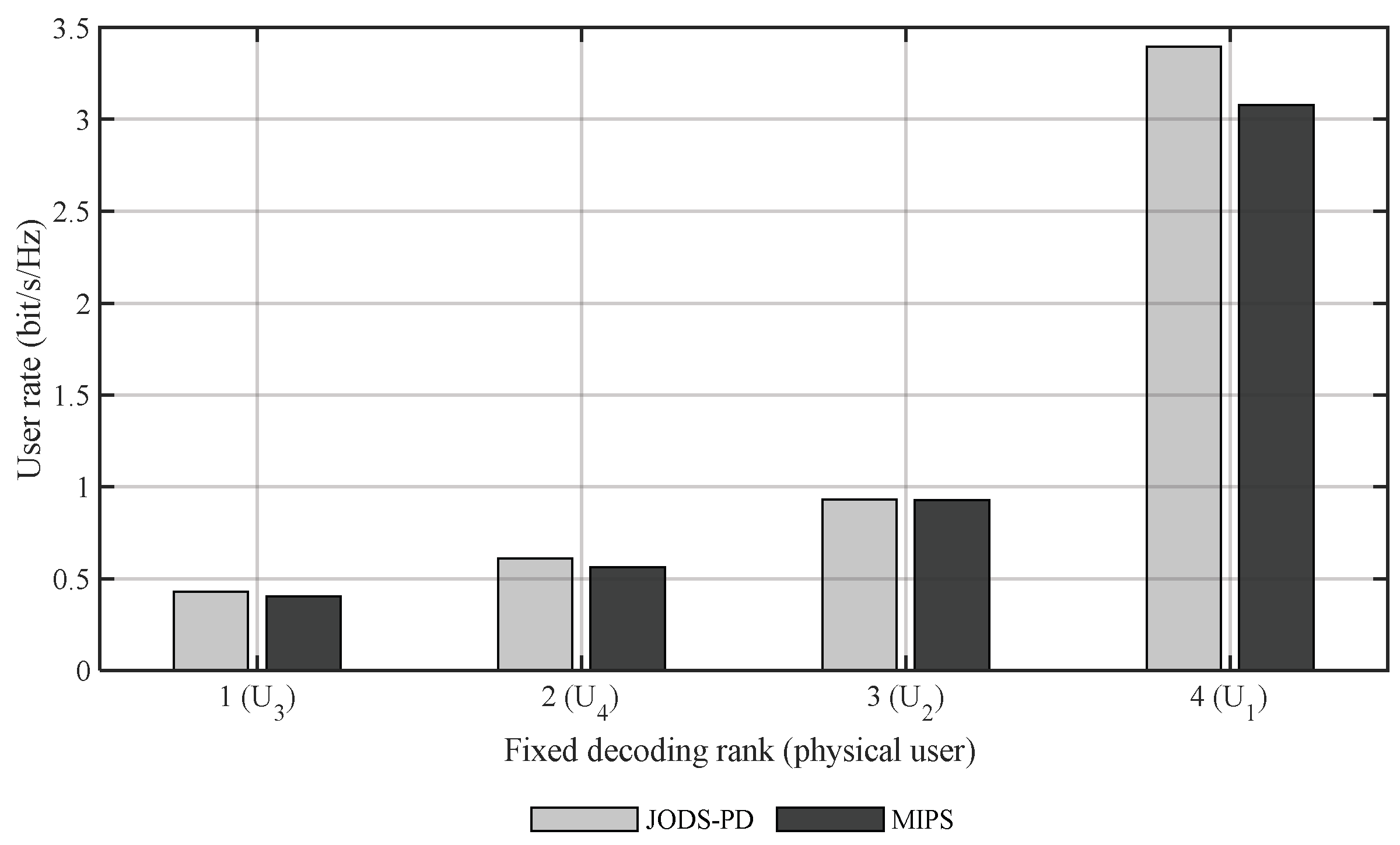
User-rate allocation for seed 42, sorted by the fixed decoding rank. Grayscale-safe bars distinguish JODS-PD and MIPS; the distribution reflects the sum-rate objective without explicit minimum-rate constraints.
Figure 5.
User-rate allocation for seed 42, sorted by the fixed decoding rank. Grayscale-safe bars distinguish JODS-PD and MIPS; the distribution reflects the sum-rate objective without explicit minimum-rate constraints.
Figure 6.
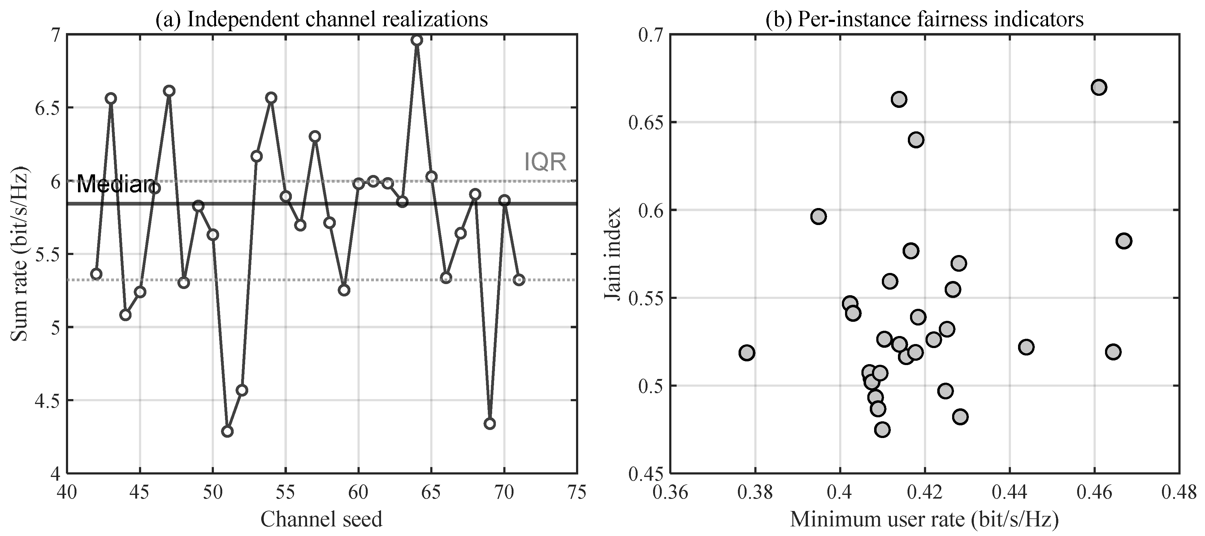
Thirty-channel JODS-PD results. (a) Returned sum rates with the median and interquartile-range boundaries; (b) per-instance Jain index versus minimum-user rate.
Figure 6.
Thirty-channel JODS-PD results. (a) Returned sum rates with the median and interquartile-range boundaries; (b) per-instance Jain index versus minimum-user rate.
Figure 7.
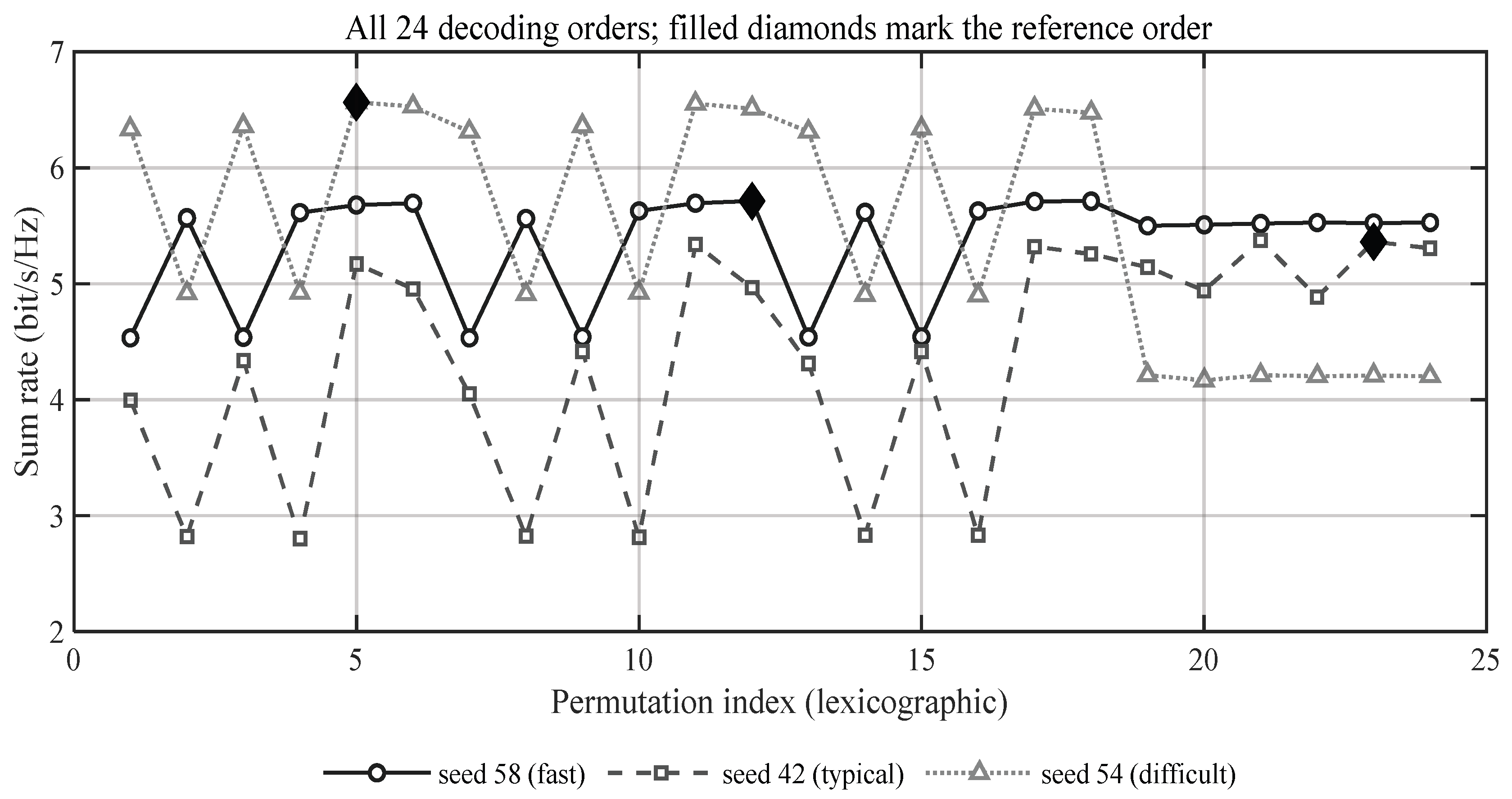
Decoding order sensitivity for seeds 58, 42, and 54. The three curves show the returned sum rates across all 24 permutations and identify the prescribed reference order.
Figure 7.
Decoding order sensitivity for seeds 58, 42, and 54. The three curves show the returned sum rates across all 24 permutations and identify the prescribed reference order.
Figure 8.
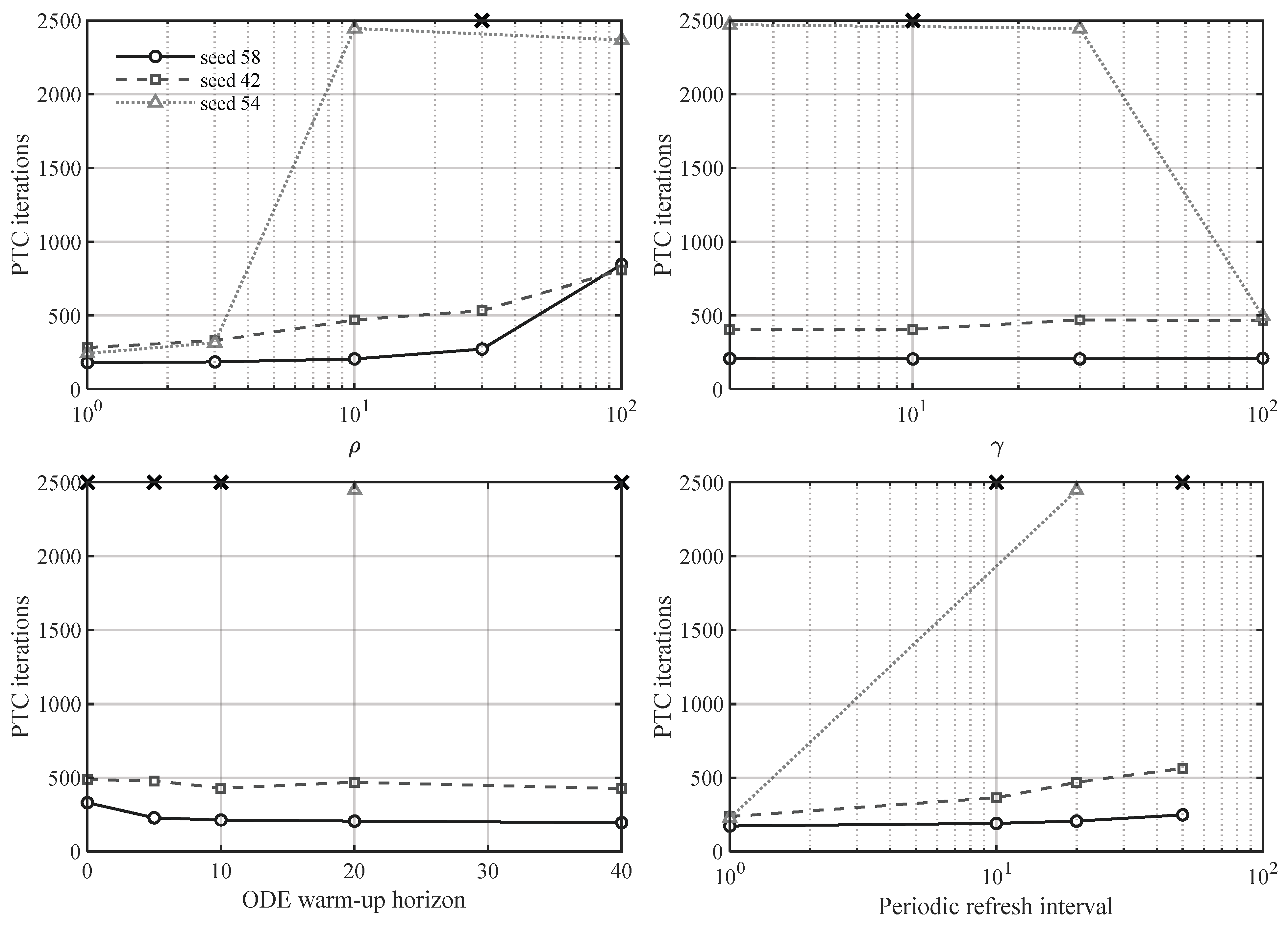
Parameter sensitivity of the PTC iterations. Solid, dashed, and dotted curves represent seeds 58, 42, and 54, respectively. Crosses indicate unsuccessful runs, while light-gray solid and dotted vertical lines denote major and minor gridlines, respectively.
Figure 8.
Parameter sensitivity of the PTC iterations. Solid, dashed, and dotted curves represent seeds 58, 42, and 54, respectively. Crosses indicate unsuccessful runs, while light-gray solid and dotted vertical lines denote major and minor gridlines, respectively.
Figure 9.
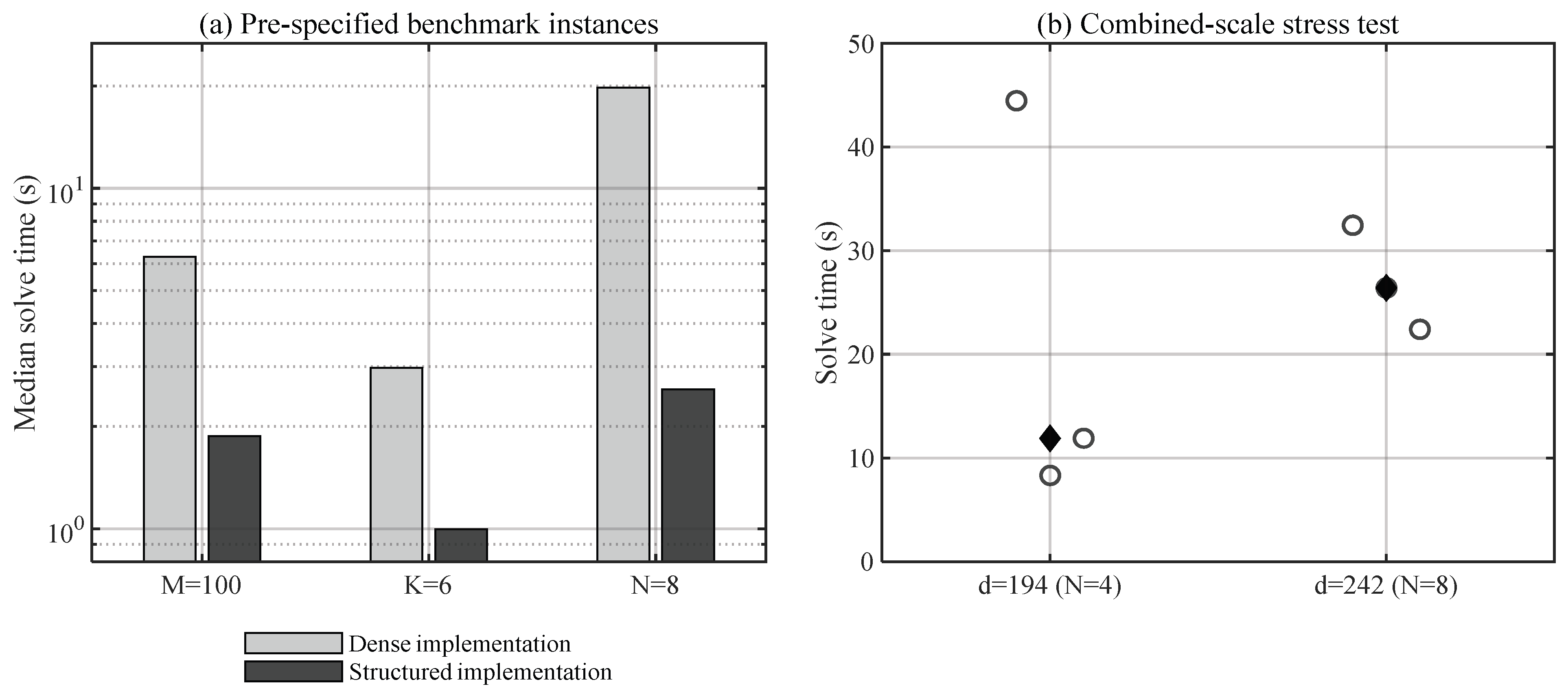
Effects of structured Jacobian assembly and inactive multiplier elimination. (a) Median solver time for the pre-specified M = 100, K = 6, and N = 8 one-factor instances; (b) per-run solver time for the combined d = 194 and d = 242 stress tests. In panel (b), open circles represent individual runs, and filled diamonds indicate the median solve times.
Figure 9.
Effects of structured Jacobian assembly and inactive multiplier elimination. (a) Median solver time for the pre-specified M = 100, K = 6, and N = 8 one-factor instances; (b) per-run solver time for the combined d = 194 and d = 242 stress tests. In panel (b), open circles represent individual runs, and filled diamonds indicate the median solve times.
Figure 10.
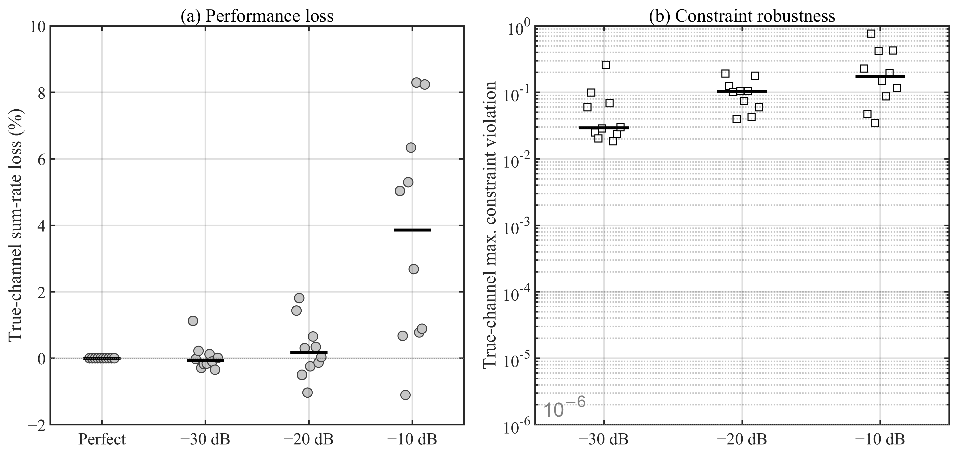
Imperfect CSI stress test. (a) True-channel sum-rate change relative to the perfect-CSI reference; (b) maximum true-channel constraint violation at −30, −20, and −10 dB NMSE. Horizontal bars indicate medians. Circles in panel (a) represent individual true-channel sum-rate losses, while squares in panel (b) represent individual maximum constraint violations.
Figure 10.
Imperfect CSI stress test. (a) True-channel sum-rate change relative to the perfect-CSI reference; (b) maximum true-channel constraint violation at −30, −20, and −10 dB NMSE. Horizontal bars indicate medians. Circles in panel (a) represent individual true-channel sum-rate losses, while squares in panel (b) represent individual maximum constraint violations.
Table 1.
Positioning of the compared numerical approaches.
Table 1.
Positioning of the compared numerical approaches.
| Approach | Variable Update | IRS and Constraints | Endpoint/Theory Statement | Main Implementation Burden |
|---|
| Representative IRS–NOMA AO/SCA/SDR | Alternating or block sequential | Relaxation/approximation with block constraints | Typically block-stationary or locally stationary under method-specific assumptions | Repeated convex/subproblem solves and recovery |
| MATPOWER Interior Point Solver (MIPS) | All variables in a generic interior-point NLP | Explicit nonlinear constraints | Solver termination and returned primal feasibility | Generic KKT factorization; scaling depends on formulation |
| AO-IPOPT | Two exact nonlinear blocks | Angle-parameterized IRS; exact block constraints | Outer convergence and primal feasibility; block-stable endpoint | Repeated exact-derivative IPOPT solves |
| JODS-PD | Simultaneous primal–dual state | Angle coordinates and adjacent ordering | Equilibrium–KKT equivalence and local transverse attraction of the KKT set | Active-set semismooth PTC and endpoint KKT audit |
Table 2.
System and channel parameters used in the matched benchmark.
Table 2.
System and channel parameters used in the matched benchmark.
| Parameter | Value |
|---|
| BS antennas, | 2 |
| IRS elements, | 30 |
| Users, | 4 |
| BS location | m |
| IRS location | m |
| User region | radius-3 m disk centered at m |
| Transmit power, | 10 dBm ( W) |
| Reference path gain, | dB at 1 m |
| Path-loss exponents, | |
| Rician factors, | 3 dB |
| Bandwidth, | 1 MHz |
| Noise power spectral density | dBm/Hz |
| Linear noise power spectral density, | W/Hz |
| Noise power, | W |
| Independent channel realizations | 30 independent channel realizations; seeds 42–51 used for matched solver comparisons |
Table 3.
Principal numerical settings for JODS-PD and MIPS.
Table 3.
Principal numerical settings for JODS-PD and MIPS.
| Setting | JODS-PD | MIPS |
|---|
| Penalty/dual gain | , | — |
| Stiff warm-up | ode15s on ; 300 event-call cap, optionally extended by 500 | — |
| Warm-up tolerances | RelTol , AbsTol | — |
| Warm-up maximum step | MATLAB default | — |
| Pilot-residual extension threshold | | — |
| PTC scaling | , | — |
| Generalized-derivative refresh | 20 steps, plus active-set and near-solution refreshes | Exact callbacks every iteration |
| Equilibrium stopping rule | or | — |
| Iteration/time limit | 2500 PTC steps | 500 interior-point iterations |
| Nonlinear feasibility/optimality tolerances | — | |
| Step control | Nonmonotone SER update | Enabled |
| Hessian regularization | None | |
Table 4.
Representative convergence and generalized Jacobian refresh statistics.
Table 4.
Representative convergence and generalized Jacobian refresh statistics.
| Case | Seed | PTC Iterations | Scheduled | Active-Set | Near-Root | Final ||F||∞ |
|---|
| Fast | 58 | 206 | 11 | 0 | 5 | 1.54 × 10⁻⁸ |
| Typical | 42 | 470 | 24 | 47 | 8 | 5.30 × 10⁻⁹ |
| Slow | 48 | 774 | 39 | 102 | 13 | 2.17 × 10⁻⁸ |
| Difficult | 54 | 2446 | 123 | 2237 | 5 | 2.79 × 10⁻¹¹ |
Table 5.
Matched comparison over seeds 42–51.
Table 5.
Matched comparison over seeds 42–51.
| Metric | JODS-PD | AO-IPOPT | MIPS |
|---|
| Successful endpoints/10 | 10 | 10 | 8 |
| Median sum rate on 8 common successes (bit/s/Hz) | 5.7285 | 5.6923 | 5.2145 |
| Median KKT/stationarity residual on common successes | <10−6 | approximately 7 × 10⁻³ (reconstructed full KKT) | method-dependent |
| Update architecture | simultaneous primal–dual | two-block alternating | generic interior point |
| Returned endpoint interpretation | low-residual KKT point | primal feasible block-stable point | primal feasible solver endpoint |
Table 6.
Distributional and user-level statistics for 30 JODS-PD channel realizations.
Table 6.
Distributional and user-level statistics for 30 JODS-PD channel realizations.
| Metric | Mean ± Standard Deviation | Median [IQR] | Range |
|---|
| Sum rate (bit/s/Hz) | 5.7073 ± 0.6307 | 5.8420 [5.3259, 5.9919] | [4.2867, 6.9603] |
| Minimum-user rate (bit/s/Hz) | 0.4188 ± 0.0193 | 0.4148 [0.4085, 0.4251] | [0.3780, 0.4669] |
| Jain index | 0.5399 ± 0.0498 | 0.5248 [0.5072, 0.5582] | [0.4749, 0.6698] |
| PTC iterations | 582.0 ± 391.8 | 500 [398.75, 661] | [207, 2447] |
| Solver time (s) | 0.5531 ± 0.9259 | 0.3901 [0.2816, 0.4518] | [0.1670, 5.3594] |
Table 7.
Symmetry-aware endpoint diagnostics over seeds 42–51.
Table 7.
Symmetry-aware endpoint diagnostics over seeds 42–51.
| Diagnostic | Observed Range/Count | Connection to Theorem 1 |
|---|
| Minimum quotient Hessian eigenvalue | 9.02 × 10⁻⁵ to 1.88 × 10⁻³ | positive curvature on tested quotient-critical subspaces |
| Transverse spectral abscissa | −1.88 × 10⁻³ to −8.91 × 10⁻⁵ | negative real parts in the complementary subspace |
| Phase-tangent residual | at most 1.56 × 10⁻⁹ | numerical invariance of the phase orbit |
| Active-rank deficiency | 1 or 2 | nontrivial multiplier fiber tangent directions |
| Observed zero modes | equal to predicted tangent dimension in all 10 cases | phase orbit plus multiplier fiber neutrality |
| Borderline curvature case | seed 49 | small but positive transverse margin |
Table 8.
Exhaustive order enumeration on three representative channels.
Table 8.
Exhaustive order enumeration on three representative channels.
| Seed | Reference Order Rank | Successful Order Sum-Rate Range (bit/s/Hz) | Interpretation |
|---|
| 58 | 1/24 | 4.5329–5.7122 | reference policy attains the best successful order |
| 42 | 2/24 | 2.8028–5.3747 | one alternative order is better |
| 54 | 1/24 | 4.2027–6.5651 | reference policy attains the best successful order |
Table 9.
Fixed-order multi-start results.
Table 9.
Fixed-order multi-start results.
| Seed | Successful Starts | Returned Sum-Rate Range (bit/s/Hz) | Within-Cluster Numerical Gap |
|---|
| 42 | 6/6 | 5.3248421–5.3620263 | 7.4 × 10⁻¹⁰% |
| 47 | 6/6 | 6.6135325–6.6135325 | 7.5 × 10⁻¹²% |
| 54 | 6/6 | 6.5651223–6.5651223 | 3.5 × 10⁻¹¹% |
Table 10.
Summary of the parameter sensitivity study (three channels per setting).
Table 10.
Summary of the parameter sensitivity study (three channels per setting).
| Parameter | Tested Values | Observed Successful Runs | Main Numerical Observation |
|---|
| Penalty ρ | 1, 3, 10, 30, 100 | 2/3 to 3/3 | ρ = 100 gives median 847 iterations |
| Dual gain γ | 3, 10, 30, 100 | 2/3 to 3/3 | changes time-scale balance and conditioning |
| Warm-up length | 0, 5, 10, 20, 40 | 2/3 to 3/3 | a short warm-up reduces poor initial branch models |
| Jacobian period | 1, 10, 20, 50 | 2/3 to 3/3 | seed 54: 2446 to 227 iterations at period 1 |
| Flow/KKT tolerance | 10−6, 10−7, 10−8 | 3/3 for each | endpoint residuals track the requested tolerance |
Table 11.
Structured JODS-PD on selected finite-size instances.
Table 11.
Structured JODS-PD on selected finite-size instances.
| N | M | K | State Dimension d | Successes | Median Solver Time (s) |
|---|
| 2 | 100 | 4 | 135 | 3/3 | 1.87 |
| 2 | 30 | 6 | 100 | 3/3 | 1.00 |
| 8 | 30 | 4 | 113 | 3/3 | 2.57 |
| 4 | 100 | 6 | 194 | 3/3 | 11.91 |
| 8 | 100 | 6 | 242 | 3/3 | 26.40 |
Table 12.
Imperfect CSI evaluation on ten channels per NMSE level.
Table 12.
Imperfect CSI evaluation on ten channels per NMSE level.
| NMSE (dB) | Estimated Problem Convergence | Median Raw Sum-Rate Change | Median True Max. Violation | Order Changes |
|---|
| −30 | 10/10 | −0.061% | 2.93 × 10⁻² | 2/10 |
| −20 | 10/10 | 0.169% | 1.03 × 10⁻¹ | 1/10 |
| −10 | 10/10 | 3.858% | 1.73 × 10⁻¹ | 8/10 |
Table 13.
CSI acquisition choices and their interaction with JODS-PD.
Table 13.
CSI acquisition choices and their interaction with JODS-PD.
| CSI Route | Information Supplied To Optimizer | Principal Advantage | Principal Design Issue |
|---|
| Explicit pilot-based estimation | direct and cascaded channel estimates with error statistics | physical interpretability and compatibility with robust constraints | training overhead increases with IRS/user dimensions |
| Implicit/learning-assisted acquisition | features, effective channels, or direct configuration proposals | potentially lower online estimation latency | training coverage, generalization, and uncertainty calibration |
| Present paper | one quasi-static channel estimate per optimization block | isolates primal–dual numerical behavior | acquisition overhead excluded; robustness assessed only by stress test |